Development of an Operating Room Scheduling Support Information System.

(1)

ABSTRACT

LI, YUE. Development of an Operating Room Scheduling Support Information System. (Under the direction of Thom Hodgson and Javad Taheri.)

The dissertation focuses on development of an operating room (OR) scheduling support information system based on the study of a Veterans Affairs (VA) medical center. On one hand, there is a need for developing such a system which is smart enough to perform necessary data analysis, incorporate the analytical results with users’ decisions, provide assistance and guidance for users in making daily OR schedules or preventing disorder due to personnel planned absence. On the other hand, the VA hospitals, due to their special role and administration policy, have many unique characteristics, e.g. budget control instead of profit driven, that should be addressed differently from the other medical environments that have been discussed in the literature.

(2)

Incorporating users’ need with the studies on data analysis, simulation and scheduling, we design a multi-user OR scheduling support information system that caters to different types of users based on their roles in the hospital.

(3)

(4)

Development of an Operating Room Scheduling Support Information System

by Yue Li

A dissertation submitted to the Graduate Faculty of North Carolina State University

in partial fulfillment of the requirements for the Degree of

Doctor of Philosophy

Operations Research

Raleigh, North Carolina

2013

APPROVED BY:

Stephen Roberts Russell King

Thom Hodgson

Co-chair of Advisory Committee

Javad Taheri

(5)

DEDICATION

(6)

BIOGRAPHY

(7)

ACKNOWLEDGEMENTS

First, I would like to thank my advisor, Dr. Thom Hodgson and Dr. Javad Taheri, for their profound ingenuity, patient guidance, and continuous encouragement. It is truly an honor to have them as my mentors, who care for students, and are always there when I need advice and guidance. Dr. Hodgson is a brilliant, knowledgeable, and humorous person, who is really pleasure to work with. I am grateful that he not only provided with me great academical ideas, taught me ways of learning and thinking, but also shared many philosophy of life that I will benefit throughout my whole life. Dr. Taheri is the one who brought us to this application area, coordinated with the VA medical center, extracted information we needed, and provided us with plenty of field insights. I am thankful that he made lots of efforts in this project, shared many of his technical experience, and has always been a source of encouragement and enthusiasm.

My committee members, Dr Stephen Roberts and Dr. Russell King, have generously given their time and expertise to better my work. I sincerely thank them for their great contribution and their good-natured support. I also thank my previous committee member Dr. Brian Denton, who has moved to University of Michigan, for his valuable comments.

I also want to thank my colleagues in our research group, Mingchun Zhao and Michelle Glatz. I really appreciate Michelle for her efforts in classifying the raw data, actively involving in the research discussion and proof reading my proposal. She gave me good impression of American culture and has always been very friendly and easy-going.

My sincere thanks and appreciation also go to the professors in the Operations Research program, particularly Thom Hodgson, Russell King, Yahya Fathi, Shu-Cherng Fang, Reha Uz-soy, James Wilson, Brian Denton - who taught me various courses at NC State and helped me in many ways. I had the honor to work as teaching assistant for Yahya Fathi and Shu-Cheng Fang in several courses and they all turned out to be wonderful experience for me.

I would like to gratefully acknowledge the Durham VA medical center for the support of our project. I had a wonderful visit there - it was a productive as well as fun-filled experience. I also owe my thanks to SAS Institute, Inc for providing the industrial training opportunity and financing my last two years’ graduate education. I would like to take this opportunity to thank my colleagues in SAS as well. My manager Alex Chien has always been really friendly and supportive. He provided me with a flexible and comfortable working environment, shared many insights on real-world application, and gave me plenty of encouragement in finishing my research work and graduate education. My colleague Pu Wang has gave me many advices on graduate study and helped me a lot in work. Many thanks to Ying Zhu, Lan Li, Ran Liu,

(8)

and programming codes, and Song Yang for all his helps since day one of my life in the US. I also want to thank my fiance Weining Shen, who has been a tremendous source of encour-agement for the last 4 years. I thank him for his guidance and support in every sphere of life. Life in the United States would not be so easy without him.

(9)

TABLE OF CONTENTS

LIST OF TABLES . . . ix

LIST OF FIGURES . . . xi

CHAPTER 1 INTRODUCTION . . . 1

CHAPTER 2 LITERATURE REVIEW. . . 5

2.1 Uncertainty . . . 5

2.2 Scheduling . . . 6

2.3 Implementation . . . 7

CHAPTER 3 DATA ANALYSIS . . . 9

3.1 Turnover Time . . . 10

3.1.1 Estimates of Turnover Time for Different Services . . . 12

3.1.2 Impact of Major/Minor Surgeries on Turnover Time . . . 12

3.1.3 The Distribution of Turnover Time . . . 14

3.2 Procedure Duration . . . 20

3.2.1 Distribution of Procedure Duration . . . 22

3.2.2 The Learning Curve of Residents . . . 23

3.2.3 Economic Effects . . . 24

3.3 Length of Stay in PACU and ICU . . . 27

CHAPTER 4 SIMULATION . . . 29

4.1 Conceptual Model . . . 30

4.2 Model Verification and Validation . . . 36

4.3 “What-if” Simulation . . . 41

4.4 Schedule Evaluation . . . 43

CHAPTER 5 SINGLE OR SCHEDULING PROBLEM . . . 46

5.1 Static Stochastic Programming Model . . . 46

5.1.1 Notation . . . 49

5.1.2 Two-Stage Stochastic Programming Model . . . 51

5.2 Practical Method for Solving the Static Scheduling Problem . . . 54

5.3 Numerical Test . . . 56

5.4 Dynamic Scheduling Problem . . . 60

5.4.1 Procedure is Canceled or Will Finish Early . . . 61

5.4.2 Procedure Will Be Finished Late . . . 61

5.4.3 Procedure Will Be Delayed because of Resource Availability . . . 61

CHAPTER 6 SYSTEM DESIGN. . . 63

6.1 Functionality . . . 63

6.1.1 Hospital Basic Information Setting . . . 65

(10)

6.1.3 Create, View and Edit Patient Information . . . 73

6.1.4 View and Edit Priority Schedule Table . . . 75

6.1.5 Build a Schedule . . . 76

6.1.6 Evaluate Schedule . . . 84

6.1.7 View Schedule . . . 84

6.1.8 Make/View Calendar . . . 85

6.1.9 Case Tracking . . . 85

6.1.10 Historical Performance Evaluation . . . 87

6.1.11 “What if” Scenario Test . . . 88

6.2 Multi-User Design . . . 88

6.2.1 Administrator’s Menu . . . 89

6.2.2 Scheduler’s Menu . . . 90

6.2.3 Physician’s Menu . . . 91

6.2.4 Nurse’s Menu . . . 92

CHAPTER 7 TWO STAGE STOCHASTIC PROGRAMMING MODEL WITH LINKING CONSTRAINTS . . . 94

7.1 Problem Definition . . . 94

7.2 Two-Stage L-Shaped Algorithm . . . 95

7.3 Convergence of the Algorithm . . . 98

7.4 Numerical Experiments . . . 102

CHAPTER 8 CONCLUSIONS AND FUTURE WORK . . . .106

REFERENCES . . . .110

APPENDICES . . . .113

Appendix A Solving for Parameters in Turnover Time Models . . . 114

A.1 Models for Matching Moments . . . 114

A.1.1 1-Uniform + Exponential . . . 114

A.1.2 1-Uniform + Erlang2 . . . 115

A.1.3 1-Uniform + Hypoexponential2 . . . 115

A.1.4 1-Uniform + Lognormal . . . 116

A.1.5 Sym-Triangular +Exponential . . . 117

A.1.6 Sym-Triangular +Erlang2 . . . 117

A.1.7 Sym-Triangular +Hypoexponential2 . . . 118

A.1.8 Sym-Triangular +Lognormal . . . 119

A.1.10 2-Uniform + Erlang2 . . . 121

A.1.11 2-Triangular + Exponential . . . 121

A.1.12 2-Triangular + Erlang2 . . . 122

A.2 Models for Matching CDF . . . 123

A.2.2 1-Uniform + Erlang2 . . . 124

(11)

(12)

LIST OF TABLES

Table 3.1 Sample Summary for Time Gap and Filtered Time Gap (in the unit of

minute) . . . 11

Table 3.2 Estimates for Expected Turnover Time . . . 12

Table 3.3 Number of Observations in the Samples . . . 16

Table 3.4 P-value in Kolmogorov-Smirnov Test for 12 Different Models by Matching Moments . . . 17

Table 3.5 P-value in Chi-Square Test for 12 Different Models by Matching Moments 17 Table 3.6 P-value for Kolmogorov-Smirnov Test for 12 Different Models by Matching CDF . . . 18

Table 3.7 P-value for Chi-Square Test for 12 Different Models by Matching CDF . . 19

Table 3.8 Number of Observations in the Samples After filtering . . . 19

Table 3.9 P-value for Kolmogorov-Smirnov Test for 12 Different Models by Matching Moments after Filtering . . . 20

Table 3.10 P-value for Chi-Square Test for 12 Different Models by Matching Moments after Filtering . . . 20

Table 3.11 P-value for Kolmogorov-Smirnov Test for 12 Different Models by Matching CDF Using the Filtered Samples . . . 21

Table 3.12 P-value for Chi-Square Test for 12 Different Models by Matching CDF Using the Filtered Samples . . . 21

Table 3.13 Best-fit Distribution for the Procedure Duration of Several Services . . . . 22

Table 3.14 Some Statistics about Procedure Durations in Orthopedics . . . 23

Table 3.15 Best-fit Distribution for the Procedure Duration of Several Orthopedics Procedures . . . 23

Table 3.16 Some Statistics about LoS in PACU for Orthopedics . . . 27

Table 4.1 Some Examples Taken from Historical Data . . . 37

Table 4.2 Computed Statistics for the Examples . . . 38

Table 4.3 97.5 % Confidence Interval for Some Statistics in Simulation with 1000 Replications . . . 39

Table 4.4 Relative Error for Some Statistics in Simulation with 1000 Replications . . 39

Table 4.5 Statistics Comparison between Simulation and Actual Realization . . . 41

Table 4.6 Statistics Comparison for Different OR Operating Hours . . . 42

Table 4.7 Statistics Comparison for Different Patient Arrival Policies . . . 43

Table 5.1 Indices . . . 49

Table 5.2 Parameters . . . 49

Table 5.3 First Stage Decision Variables . . . 50

Table 5.4 Second Stage Decision Variables . . . 51

Table 5.5 Comparison between the Practical Solution and the Optimal Solution for the Original Order Case . . . 57

(13)

Table 5.7 Comparison between the Practical Solution and the Historical Solution for

the Original Order Case . . . 58

Table 5.8 Comparison between the Practical Solution and the Optimal Solution for the Re-Order Case . . . 58

Table 5.9 Simulation Results Comparison between Threes Solutions for the Re-Order Case . . . 59

Table 5.10 Comparison between the Practical Solution and the Historical Solution for the Re-Order Case . . . 59

Table 7.1 Numerical Test Results for Newsvendor Problem . . . 104

Table B.1 Parameters . . . 126

(14)

LIST OF FIGURES

Figure 1.1 System Structure . . . 4

Figure 3.1 Illustration of Filtered Time Gap . . . 10

Figure 3.2 Workflow for Getting the Time Gap and the Filtered Time Gap . . . 11

Figure 3.3 Bubble Plot for Filtered Time Gap . . . 13

Figure 3.4 Bubble Plot for Log Transform of Filtered Time Gap . . . 14

Figure 3.5 Components of Time Gaps between Consecutive Procedures . . . 15

Figure 3.6 Histogram of Time Gaps between Consecutive Orthopedics Procedures . . 15

Figure 3.7 Histogram and Fitted Curve for Procedure Duration of Procedures with CPT Code 27447, 27130 and 29881 . . . 24

Figure 3.8 Average Procedure Duration Each Year for Procedures with CPT Code 66984 Based on 2238 Observations . . . 25

Figure 3.9 Average Procedure Duration Each Year for Procedures with CPT Code 27447 Based on 331 Observations . . . 26

Figure 3.10 Correlation between Procedure Duration and LoS in the PACU . . . 28

Figure 4.1 Simulation Process Illustration . . . 31

Figure 4.2 Main Simulation Process Flowchart . . . 33

Figure 4.3 Simulation Example E5 Illustration . . . 40

Figure 4.4 Simulation Process Flowchart for Schedule Evaluation . . . 45

Figure 5.1 Illustration of Idle Time, Waiting Time and Overtime . . . 47

Figure 5.2 Illustration of a Case that Should Not Happen . . . 48

Figure 5.3 Expected Number of Procedures Scheduled Per Schedule Block over Dif-ferent Values ofα . . . 60

Figure 6.1 System Work Flow . . . 64

Figure 6.2 Contents for Input Table “History” . . . 65

Figure 6.3 Contents for Input Table “PatientMovement” . . . 65

Figure 6.4 Hospital Basic Information Setting From . . . 66

Figure 6.5 System Settings Form . . . 68

Figure 6.6 Schedule Settings Form . . . 69

Figure 6.7 Service Setup Form . . . 70

Figure 6.8 OR Setup Form . . . 71

Figure 6.9 Physicians Setup Form . . . 71

Figure 6.10 Nurses Setup Form . . . 72

Figure 6.11 Test Schedule Settings Form . . . 72

Figure 6.12 Test Schedule Settings - View Results Form . . . 73

Figure 6.13 Patient Information Form . . . 74

Figure 6.14 CPT Finder Form . . . 75

Figure 6.15 Edit Priority Schedule Table Form . . . 76

Figure 6.16 View Priority Schedule Table Form . . . 76

(15)

Figure 6.18 Build Initial Schedule - Add Procedures Manually . . . 78

Figure 6.19 Build Initial Schedule - Edit Information . . . 79

Figure 6.20 Build Initial Schedule - Send List to Scheduler . . . 79

Figure 6.21 Build Schedule - Add Procedures . . . 80

Figure 6.22 Build Schedule - Generate Schedule Automatically . . . 81

Figure 6.23 Build Schedule - View Generated Schedule and Expected Performance . . 82

Figure 6.24 Build Schedule - View Schedule and Evaluation Results . . . 82

Figure 6.25 Build Schedule - Edit/Publish Schedule . . . 83

Figure 6.26 View Multiple Block Schedule Evaluation Results . . . 84

Figure 6.27 View Published Schedule . . . 84

Figure 6.28 Make/View Calendar From . . . 85

Figure 6.29 Update Case Status Form . . . 86

Figure 6.30 Check OR Status Form . . . 87

Figure 6.31 Historical Performance Evaluation and “What if” Test Form . . . 88

Figure 6.32 Login Form . . . 89

Figure 6.33 Main Menu for Administrators . . . 90

Figure 6.34 Main Menu for Schedulers . . . 91

Figure 6.35 Main Menu for Physicians . . . 92

(16)

CHAPTER 1

INTRODUCTION

The Veterans Health Administration is home to the United States’ largest integrated health care system consisting of 152 medical centers, nearly 1,400 community-based outpatient clinics, community living centers, Vet Centers, and Domiciliaries. They provide comprehensive care to the 22 million veterans, serving more than 8.3 million veterans each year. Most of the Veterans Affairs (VA) Medical Centers operate in a similar way. Most offer medical and surgical specialty services including audiology and speech pathology, dermatology, dental, geriatrics, neurology, oncology, podiatry, prosthetics, urology, and vision care. Some also offer advanced services such as organ transplants and plastic surgery. Most VA medical centers are adjacent to medical schools whose faculty and residents perform services at the centers.

The problem to be studied is that of scheduling operating rooms (OR) at the Durham VA Medical Center. The Medical Center serves veterans in central and eastern North Carolina in its main medical center or one of its three community-based outpatient clinics. Services are available to more than 200,000 veterans living in a 26-county area. Because of the large demand for surgical services, the VA is trying to increase throughput in the OR’s.

In this hospital, most of the surgical procedures done are elective. The procedures can be categorized into fourteen different service types: Cardiac, General, Gynecology, Neurology, NSU, Otolaryngology Head and Neck Surgery (OHNS), Ophthalmology, Oral, Orthopedics, Plastic, Podiatry, Thoracic, Urology, and Vascular. There are eight ORs in the hospital. The standard operating hours for OR1 and OR2 are 10 hours per day, and eight hours per day for OR3 through OR8. The service type for each schedule block (a combination of date and room, e.g. Oct. 5th morning in OR 1) is predetermined according to a “Priority Schedule Table” made by the hospital two months in advance.

(17)

plan to do and submit it to the scheduler. In the desired schedule, they state which patient is first, second, and so on. The scheduler estimates the duration of each surgery based on the average historical duration of that procedure in their system, the surgical team (how well the team works together, or if resident physicians are involved which increases the duration because of the teaching process, etc.). The scheduler may also consider the surgeon’s estimate of time needed. However, he/she believes that they always underestimate the time, and their estimates are mainly the time from the incision to closing. The time the scheduler posts in the schedule is for the time from patient in to patient out, so the scheduler has to add at least half an hour to the surgeon’s estimate. The scheduler’s time estimate is usually in 30 minute units (e.g., 1 hour 30 minutes or 2 hours), the best they can do will be in 15-minute segments. Based on the sequence and estimated duration of each surgery, the scheduler builds a schedule, and then negotiates with each surgeon until they agree with the sequence and a planned start time/end time for each surgery. If there is any change to the planned schedule, they notify the patient. By 1pm on the day before the surgery, the scheduler posts a schedule. It includes the procedure, the room, the time (e.g., 8:00-12:00), surgeon, etc. The scheduled start time of the first procedure is 9 am on Wednesdays and 8 am for all other days. The scheduled turnover time between two surgeries is 30 minutes.

(18)

Post Anesthesia Care Unit (PACU) and tells them to bring the a bed into the OR. If there is no bed in the PACU, the patient must wait in the OR after the surgery. When the closing is done, the anesthetist starts to wake the patient up. Most of the patients are moved to the PACU for at least one hour for really waking up. Then they are taken into the ward, Intensive Care Unit (ICU) or home. After the patient leaves the OR, the nurses turnover the OR and then set up for the next surgery.

If the first surgery ends early and the next patient is ready, the surgical team starts the next one earlier than planned. So the scheduled start time is really a guideline instead of a rule. If the next to last surgery planned for the day ends later than the OR close time, the surgical team decides whether they will continue to do the last one. But since most of the surgeries are elective, they usually just cancel it.

The daily OR schedules are manually created by a “scheduler”. Our objective is to develop an information system to assist the staff in making daily schedules for the ORs. The system should provide performance evaluation corresponding to each schedule, so that the scheduler can foresee the effects of the schedule and adjust scheduling decisions accordingly. It should also provide suggestions for improving the schedule. When the regular “scheduler” is on leave, the system should be able to provide some help in OR scheduling to avoid disorder.

As an application problem, the challenges come from three perspectives: accuracy, efficiency and the ability to generalize. First, the model we build to describe the system, needs to be as accurate as possible. It is driven by both the cost of running the ORs and the demands for increasing throughput. Uncertain surgical durations, patients’ recovery time, etc. increase the uncertainty of the whole process, so we need to perform a thorough analysis of the data to reduce the inaccuracy in describing the process. In addition, the availability of different resources like personnel and critical equipment complicate the process more. Thus a simulation model that takes into consideration the impact of different resource’s availability should be built. The model will never behave exactly like reality, so we need to find a balance between a high level of detail and the ease of handling the model. Second, the system should meet the users’ need and provide a practical solution. We should understand the factors users need to consider when they are making scheduling decisions and provide them with corresponding reliable information. This requires a significant amount of model validation and user involvement. In this paper, as the early stage of our study, we were not able to show the effect of the study, so the system is designed based on our current understanding of the needs. With improved understanding, the system will be adjusted to achieve this goal. Last but not least, the method we propose should be able to be generalized to other situations even though this is a scenario based study.

(19)

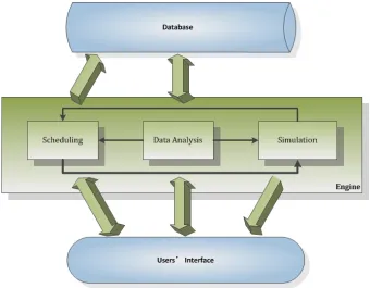
Figure 1.1: System Structure

Combining the information obtained from the users’ interface with the data stored in the database, data analysis can be performed. Based on the results of data analysis, users can make schedules. The simulation will provide performance analysis for schedules. Users can adjust their schedules based on the simulation results. The system can also automatically generate schedules. Then the information and schedules will be stored in the database for future use.

(20)

CHAPTER 2

LITERATURE REVIEW

Operating rooms, where about 42% of a hospital’s revenue is generated [HFMA, 2003], have received increasing attention over the years. Based on a comprehensive literature review per-formed by [Cardoen et al., 2010], there are 247 references relevant to operating room planning and scheduling. The following reviews focus on three aspects: uncertainty, scheduling and im-plementation.

2.1 Uncertainty

The uncertainty inherent in surgical service times is a major issue in the development of ac-curate operating room schedules. Among the literature addressing uncertainty, modeling the surgical case duration is the most widely studied problem. [Wright and Bonar, 1996] showed that combining surgeons’ estimates and prior case duration data together outperforms either used separately. [Hancock et al., 1988] introduced a methodology to provide procedure times based on a historical data base. The data is first subdivided by code, primary (staff) surgeon, case teaching status, patient inpatient/outpatient status, patient sex, patient age, etc. Then rules, testing and pooling are introduced to further cluster the data. [Dexter et al., 2008] sys-tematically reviewed the articles reporting statistically significant differences in preoperative times with the specialty of general thoracic surgery, which is a typical specialty of elective surgery. They concluded that it is important to rely on the precise procedure(s), surgical team, and type of anesthetic when estimating case durations. These works provide us with sugges-tions on the factors that potentially have impact on procedure durasugges-tions. Since OR times differ greatly for the same procedure in different hospitals [Dexter et al., 2006], we need to identify factors crucial to predict procedure durations in our case.

(21)

not valid in practice. Turnover time should be considered as a service specific random vari-able. Some work has modeled the turnover time differently. [Marcon et al., 2003] considered the surgical preparation duration and clean-up duration to be dependent on the specialty. [Marcon and Dexter, 2007] adopted both a bounded two parameter Lognormal distribution and a constant.

As for Length of Stay (LoS) in the PACU, there are fewer studies using different methods. [Marcon and Dexter, 2006] assumed scheduled OR times, turnover times and PACU LoS are different for different services, and they follow Lognormal distributions but are also bounded. The PACU LoS in [Marcon et al., 2003] ’s work were estimated by the anesthesiologists and the OR manager. They were dependent on range of surgical case duration and the results were mentioned to be in accordance with a statistical analysis conclusion that PACU LoS was 46% of the total length of anesthesia, which was obtained from a 2-year database in a French public hospital. Analysis about general surgery in [VanBerkel and Blake, 2007] showed that there is a statistical difference of LoS between elective patients, non-elective patients, and non-surgery pa-tients, and LoS was statistically different for some categories. [Belin and Demeulemeester, 2007] assumed that LoS followed a Multinomial distribution with parameters which depend on the type of surgery.

2.2 Scheduling

Simulation proves to be a useful methodology for dealing with complex and stochastic problems because of its extensive modeling flexibility. It is used in many cases to study policies for operating room scheduling and resource allocation.

(22)

A few researchers dealt with an integrated operating room or simulated the entire hospital providing a systematic view. [Marcon et al., 2003] devised a simulation model to determine the minimum number of PACU beds, and investigated how factors like LoS and number of porters influence the hourly occupancy of the PACU. Their model included ORs, PACU and OR staff. The preoperative process was composed of transportation of the patient from a ward bed to the OR, anesthesia induction, surgical preparation, surgical procedure, patient’s PACU stay and transportation of the patient back to the ward. [Marcon and Dexter, 2006] used discrete event simulation to study the impact of several different surgery sequencing rules on the phase I PACU staffing and over-utilized OR time resulting from delays in PACU admission. The best rules were shown to be those that smooth the flow of patients entering the PACU. In their model, they assumed the actual OR time of each case to be equal to the scheduled OR time multiplied by a normally distributed random number with a mean of 1 and standard deviation of 0.25. [Denton et al., 2006] applied a Monte-Carlo simulation model and simulated annealing to schedule a multi-OR surgical suite. The process in the simulation included intake, surgery and recovery. [Baumgart et al., 2007] proposed a conceptual framework of using computer sim-ulations in different stages of the business process management lifecycle for operating room management.

As for optimization methods in OR scheduling problems, many previous research works adopt deterministic models. [Aida Jebalia, 2006] developed a two-step Mixed Integer Program-ming (MIP) model. The first step consists of assigning surgical operations to operating rooms. Resources including ORs, surgeon, equipment, ICU, etc. are all taken into consideration. The second step focus on sequencing the assigned operations with the objective of minimizing the total overtime in all ORs.

There are also a number of stochastic programming optimization models for OR scheduling. [Denton and Gupta, 2003] studied a single OR scheduling problem with the objective of min-imizing the total expected cost of customer waiting time, server idle time, and tardiness with respect to the session length. They developed a modified L-shaped algorithm based on derived upper and lower bounds that are independent of procedure duration type. [Denton B, 2007] described a stochastic optimization model and some practical heuristics for computing surgery sequencing and start-time decisions. [Batun et al., 2011] present a two-stage stochastic mixed integer programming model to minimize total expected operating cost for a generalized parallel operating room environment.

2.3 Implementation

(23)

sys-tem. Requests are sorted and assigned using the system according to their relative priority, which is based on the service priority, suggested time interval, surgeon priority, and room preference. [Hanson, 1982] reported a system providing procedure-specific information, special equipment reservation and availability of equipment. [Ozkarahan, 1995] introduced an expert hospital decision support system which combined mathematical programming, knowledge base, and database technologies. An enhanced version using a goal programming model was described in [Ozkarahan, 2000]. [Harper, 2002] proposed a generic framework. It features a system creating statistically and clinically meaningful patient groups using Classification and Regression Tree analysis, and estimating the parameters of statistical distributions using a simplex optimiza-tion algorithm. A simulaoptimiza-tion tool for hospital resources was also introduced. The framework was illustrated by cases drawn from a set of local hospitals. [Harper and Gamlin, 2003] ap-plied a simulation modeling approach to examine various appointment schedules in order to reduce patient waiting times in an outpatient department. [Belin et al., 2006] developed a soft-ware system that visualizes the impact of the master surgery schedule on demand for various resources throughout the hospital. And later in [Belin et al., 2009], the author presented a cor-responding decision support system relying on both a mixed integer programming technique solving multi-objective linear and quadratic optimization problems and a simulated annealing meta-heuristic.

(24)

CHAPTER 3

DATA ANALYSIS

We consider the hospital as a system centered on the ORs. There are three important processes of the OR-centered system: OR turnover, performing a surgical procedure, and patient stay in the PACU and/or ICU. The distribution of turnover time, procedure duration and LoS in the PACU and ICU are critical to simulating the whole system and generating OR schedules. We also need to give point estimates of these times so that the users can use the information for making their decisions.

Our process of understanding the system started with analyzing historical data. The records of case ID, Current Procedural Terminology (CPT) code, OR, date, patient in OR time, patient out of OR time, start time and end time of each surgical procedure performed are available. Patient movement information includes patient id, ward location, transaction (could be check in, transfer, check out, etc.), transaction times are also availabe.

The CPT code is used to describe medical, surgical and diagnostic services. Since there is no record about which service type each procedure should be categorized into, we used the CPT code to identify the service type. Six months of data (Aug. 15th 2009 - Feb. 10th 2010) was collected. The procedure names and descriptions of CPT codes were manually checked to cate-gorize the corresponding procedures into different services. The CPT code ranges corresponding to each service type were recorded. In the following study, the service for each procedure is de-termined by these identified CPT code ranges. Most of the later data analysis results are based on 4.5 years of data (from Oct. 3rd 2006 to Apr. 11th 2011) from the orthopedics service, which is a representative elective surgical service.

First, it is necessary to define some common terms:

(25)

Turnover time is the time used to prepare for the next procedure. It includes cleanup times and set up times, but not the delays between contiguous procedures in the OR. The delays may be caused by the unavailability of surgeons or critical equipment.

Length of Stay in PACU is defined as the time from when a patient enters a PACU after his/her surgical procedure until the patient leave the PACU.

In this chapter, we describe in detail how to perform data analysis to reduce the uncertainty in our description of three time related variables and show our data analysis results. The three types of time related variables are crucial to OR scheduling: turnover time, surgical procedure duration, and LoS in the PACU and the ICU.

3.1 Turnover Time

The difficulty of estimating turnover time lies in the fact that there is no direct data relative to actual turnover times. The most relevant data we have is the time gap between two consecutive procedures. The time gaps may be caused by not only the turnovers, but also the availability of surgical teams and critical equipment, patient readiness, etc.

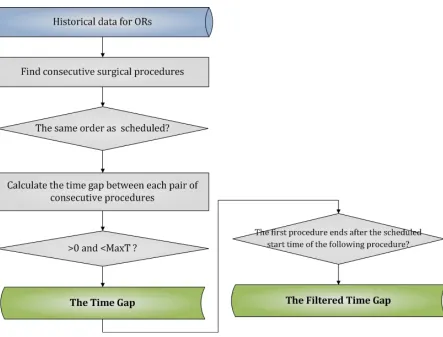
In order to get a better estimate of turnover time, we only use the type of time gap illustrated in Figure 3.1, in which the first procedure ends after the scheduled start time of the following procedure. The advantage of only using this type of time gap is that it reduces the randomness caused by the schedule. In other words, if the first procedure ends earlier than the scheduled end time, then the patient and surgical team for the following surgery may not be ready, so the time gap would be longer. The data summary of the 4.5 years’ worth of sample data for both the original time gap and the filtered time gap are listed in Table 3.1. The workflow for getting the time gap and the filtered time gap is described in Figure 3.2.

(26)

Figure 3.2: Workflow for Getting the Time Gap and the Filtered Time Gap

Table 3.1: Sample Summary for Time Gap and Filtered Time Gap (in the unit of minute)

Time Gap Filtered Time Gap Number of Observations 1065 375

Max 497 194

Mean 48.1 45.7

Standard Deviation 30.4 23.2

Coefficient of Variation 0.63 0.51

(27)

Table 3.2: Estimates for Expected Turnover Time

Service Type Cardiac Oral General Gyn Neurology

Turnover Time 60 51 15 41 35

Service Type OHNS Ophthalmology Orthopedic Plastic Podiatry

Turnover Time 33 15 30 21 45

Service Type Thoracic Urology Vascular

Turnover Time 38 25 29

turnover time based on the filtered time gap.

3.1.1 Estimates of Turnover Time for Different Services

Since the time gap is an upper bound for turnover time, the expected turnover time should be a certain percentile of the time gaps. Instinctively, the turnover time for different services (e.g. Cardiac and Ophthalmology) may be different. To estimate turnover times, we collected one month of historical data (Oct. 2009) pertaining to time gaps between two surgical procedures of the same service performed in the same OR on the same day. We use the 20th percentile of the collected data as our estimate of the expected turnover time for each service in our study (Table 3.2). Using this percentile, we are able to remove some outliers due to data entry errors and also help to remove the idle time in the time gap.

The results are quite reasonable based on verification by people working in the hospital. The flaw here is that the analysis is based on one month’s data and the 20th percentile selection is arbitrary based on the results. We also applied the same method on 5 years of historical data from orthopedics procedures, and we got the same results, 30 minutes, as shown in the table, which supports the robustness of the 20th percentile method.

We also used these results in estimating how many additional cases the hospital could schedule when they open an OR room only for minor surgeries. Since minor surgeries usually take less time, the accuracy of turnover time estimates would be more critical compared with scheduling major surgeries. Our estimates based on these results were considered reasonable to the hospital personnel, which also shows the reasonability of the turnover time estimate results in Table 3.2.

3.1.2 Impact of Major/Minor Surgeries on Turnover Time

(28)

major surgeries, the turnover time would be longer than if they are both minor surgeries. To test this hypothesis, records of Oct. 2009 were used. The surgeries were categorized into two surgery types: major and minor. According to the surgery complexity of every pair of consecutive surgeries, each turnover time was classified as one of the four turnover types: major-to-major, major-to-minor, minor-to-major and minor-to-minor. For each service, Analysis of Variance (ANOVA) was used to test the differences between expected time gaps of these four turnover types. Statistically, there was no significant difference between the expected time gaps of these four types, which implies no significant difference between the expected turnover times. This study showed that based on a limited data set, whether two surgeries are major or minor surgeries does not significantly affect the turnover time between them. However, the study was based on historical data from only one month, so further analysis using more data is needed.

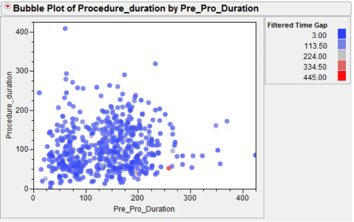
Since there is no direct record about a surgery being classified as either major or minor, lots of expert opinions from hospital staff are needed for this study. Under an assumption that major surgeries take more time and minor surgeries take less time, we can address this issue by checking the relation between the durations of two consecutive procedures and the time gap length in between. Figure 3.3 shows the bubble plot for the filtered time gap. The

Figure 3.3: Bubble Plot for Filtered Time Gap

(29)

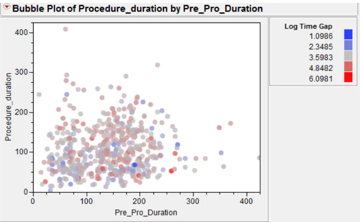
Figure 3.4: Bubble Plot for Log Transform of Filtered Time Gap

duration separately, and the color of the bubble shows the filtered time gap as explained in the legend. Since the filtered time gap has a long end tail, the choices of the color make the results not quite obvious. Thus, we take the natural logarithm transform of the filtered time gap and the corresponding results are shown in Figure 3.4. We can see that there is no obvious color pattern, which means there is no significant result showing that the procedure lengths would impact the turnover time. A linear model is also tried with the filtered time gap as the dependent variable and the two procedure durations as the explanatory variables. The p-values for the two explanatory variables are 0.9315 and 0.1188, respectively, which also supports our conclusion that procedure durations have no significant impact over the turnover time.

3.1.3 The Distribution of Turnover Time

Turnover time is a random variable (i.e. one can’t guarantee that it takes exactly 15 minutes every time, maybe it will take 13 minutes this time, and 18 minutes next time). So there is a need to model the distribution of turnover time.

(30)

proce-dures looks like the shape shown in Figure 3.6, we can compute different convolution results of the two random variables under different assumptions of distributions, and compare the results with the distribution of the time gaps. Thus, we attempt to find a reasonable distribution of the turnover time in this way.

Figure 3.5: Components of Time Gaps between Consecutive Procedures

Figure 3.6: Histogram of Time Gaps between Consecutive Orthopedics Procedures

(31)

symmetric Triangular and 2-parameter Triangular distributions. Except for the 2-parameter Uniform distribution, the remaining three distributions all use 10 minutes, which is the shortest turnover time in the historical record, as the left-side boundary. This way, we reduce the number of parameters that need to be estimated by 1.

As for the idle time, we tried well-known distributions including Exponential, 2-stage Erlang, 2-parameter Hypo-exponential and Lognormal distributions. The first two distributions contain 1 unknown parameter and the other two contain 2 unknown parameters.

We only consider the combined models with at most 3 unknown parameters. This is because in order to solve 4 parameters, we would need, at the least, information about kurtosis, which is the fourth moment, however, as we know, higher moments tend to be less accurate and robust than lower moments if we estimate them from a sample. So in our study, we do not assume the accuracy of moments higher than the third moment.

Using the moments’ information from the samples, we can estimate the parameters by solving an optimization problem. For example, for models with 3 unknown parameters, we minimize the absolute difference between the model skewness and the sample skewness, with the constraints that the mean and variance of the model equal the mean and variance of the sample. Since the feasible region is not convex, we first solve the two equations in the constraints to represent the remaining 2 parameters using the first parameter in the turnover time distribution. This way we can covert the optimization problem with 3 variables into one with only 1 variable. Since this variable is bounded, we can choose a sufficient number of initial solutions within the boundaries to develop a deepest gradient algorithm to solve the non-convex nonlinear programming problem. The details of the models are listed in Appendix A.1.

The Kolmogorov-Smirnov and Chi-Square tests are performed to test how good our models are using the filtered time gap data based on the 4.5-year of historical data. Table 3.3 shows the size of the samples, and Table 3.4 shows the p-value in the Kolmogorov-Smirnov test for each model and each sample year and Table 3.5 shows that for the Chi-Square test.

Table 3.3: Number of Observations in the Samples

Sample 2006 2007 2008 2009 2010 2011 Number of Observations 20 80 79 107 67 20

(32)

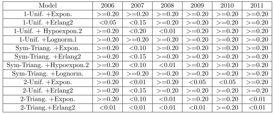
Table 3.4: P-value in Kolmogorov-Smirnov Test for 12 Different Models by Matching Moments

Model 2006 2007 2008 2009 2010 2011

1-Unif. +Expon. >=0.20 >=0.20 >=0.20 >=0.20 >=0.20 >=0.20 1-Unif. +Erlang2 <0.05 <0.15 >=0.20 >=0.20 >=0.20 >=0.20 1-Unif. + Hypoexpon.2 >=0.20 <0.20 <0.01 >=0.20 >=0.20 >=0.20 1-Unif. +Lognorm.l >=0.20 >=0.20 >=0.20 >=0.20 >=0.20 >=0.20 Sym-Triang. +Expon. >=0.20 <0.10 >=0.20 >=0.20 >=0.20 >=0.20 Sym-Triang. +Erlang2 >=0.20 <0.15 >=0.20 >=0.20 >=0.20 >=0.20 Sym-Triang. +Hypoexpon.2 >=0.20 <0.10 <0.01 >=0.20 >=0.20 >=0.20 Sym-Triang. +Lognorm. >=0.20 >=0.20 >=0.20 >=0.20 >=0.20 >=0.20 2-Unif. +Expon. >=0.20 <0.01 >=0.20 <0.05 <0.05 >=0.20 2-Unif. +Erlang2 >=0.20 <0.15 >=0.20 >=0.20 >=0.20 >=0.20 2-Triang. +Expon. >=0.20 <0.10 <0.01 >=0.20 >=0.20 <0.01 2-Triang.+Erlang2 <0.01 <0.01 <0.01 <0.01 >=0.20 <0.01

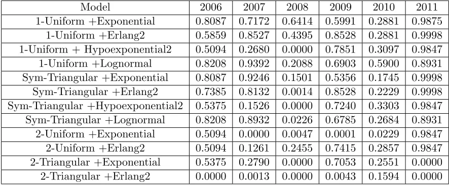
Table 3.5: P-value in Chi-Square Test for 12 Different Models by Matching Moments

Model 2006 2007 2008 2009 2010 2011

1-Uniform +Exponential 0.5375 0.3155 0.2114 0.6749 0.3303 0.6487 1-Uniform +Erlang2 0.8392 0.0732 0.0379 0.7415 0.2857 0.6487 1-Uniform + Hypoexponential2 0.5375 0.2790 0.0000 0.7053 0.2763 0.7836 1-Uniform +Lognormal 0.6692 0.6363 0.0320 0.7556 0.2029 0.6868 Sym-Triangular +Exponential 0.5494 0.1526 0.1719 0.7240 0.1745 0.8931 Sym-Triangular +Erlang2 0.5859 0.0618 0.0034 0.7143 0.2949 0.9847 Sym-Triangular +Hypoexponential2 0.5375 0.1526 0.0000 0.7240 0.1745 0.9847 Sym-Triangular +Lognormal 0.6692 0.6363 0.0690 0.7556 0.2029 0.8931 2-Uniform +Exponential 0.5375 0.0000 0.4100 0.0001 0.0229 0.7836 2-Uniform +Erlang2 0.5094 0.0732 0.4156 0.7415 0.3670 0.9847 2-Triangular +Exponential 0.5494 0.1526 0.0000 0.6387 0.1551 0.0000 2-Triangular +Erlang2 0.0000 0.0004 0.0000 0.0006 0.2857 0.0000

more parameters.

(33)

between the sample CDF values and the model CDF values. The disadvantage is that we will increase the computation time (from several minutes to a day for each sample) because there are no closed form CDFs for most models and we have to generate a set of numerical CDFs for each feasible solution for each model. The advantage is that we can get more accurate results (Table 3.6 and Table 3.7). So we can use the method if we have enough time and use the faster method that matches the higher moment when a quick result is desired. The details of the models using the closed CDF form are listed in Appendix A.2.

Table 3.6: P-value for Kolmogorov-Smirnov Test for 12 Different Models by Matching CDF

Model 2006 2007 2008 2009 2010 2011

1-Unif. +Expon. >=0.20 >=0.20 >=0.20 >=0.20 >=0.20 >=0.20 1-Unif. +Erlang2 >=0.20 >=0.20 >=0.20 >=0.20 >=0.20 >=0.20 1-Unif. + Hypoexpon.2 >=0.20 >=0.20 <0.01 >=0.20 >=0.20 >=0.20 1-Unif. +Lognorm. >=0.20 >=0.20 >=0.20 >=0.20 >=0.20 >=0.20 Sym-Triang. +Expon. >=0.20 >=0.20 >=0.20 >=0.20 >=0.20 >=0.20 Sym-Triang. +Erlang2 >=0.20 >=0.20 >=0.20 >=0.20 >=0.20 >=0.20 Sym-Triang. +Hypoexpon.2 >=0.20 <0.10 <0.01 >=0.20 >=0.20 >=0.20 Sym-Triang. +Lognorm. >=0.20 >=0.20 >=0.20 >=0.20 >=0.20 >=0.20 2-Unif. +Expon. >=0.20 <0.01 >=0.20 <0.05 <0.05 >=0.20 2-Unif. +Erlang2 >=0.20 >=0.20 >=0.20 >=0.20 >=0.20 >=0.20 2-Triang. +Expon. >=0.20 >=0.20 <0.01 >=0.20 >=0.20 <0.01 2-Triang. +Erlang2 <0.01 <0.01 <0.01 <0.01 <0.15 <0.01

Aside from the turnover and regular idle times, sometimes the filtered time gap may include some noise. For example, the time gap could be very large due to some typographical errors (typos), since the data is manually entered into the database. So we need a method to detect and remove the noisy data point. We extend the ideas of the Kalman filter [Kalman, 1960] to apply it here for modeling the distribution of turnover time. The basic steps are listed below.

Algorithm 1 Kalman Filtering for Modeling the Distribution of Turnover Time

Step 0.Let the data setDcontain the corresponding time gaps data, and Set a parameterα. Step 1. Given data setD, Find the best-fit distribution with CDFF.

(34)

Table 3.7: P-value for Chi-Square Test for 12 Different Models by Matching CDF

Model 2006 2007 2008 2009 2010 2011

For each year’s time gap data set, we setα= 0.01 and use the matching moments method in the filtering algorithm to find the best-fit distribution in each iteration. Table 3.8 shows the size of the samples after the filtering algorithm. As we can see, the number of data points filtered in each data set is between 1 and 4. Table 3.9 shows the p-value in the Kolmogorov-Smirnov test for each model and sample year and Table 3.10 shows this for the Chi-Square test. We can see that the best fitted test results are better than previous test results for the samples without the filtering.

Table 3.8: Number of Observations in the Samples After filtering

Sample 2006 2007 2008 2009 2010 2011 Number of Observations 19 77 79 106 63 18

(35)

Table 3.9: P-value for Kolmogorov-Smirnov Test for 12 Different Models by Matching Moments after Filtering

Model 2006 2007 2008 2009 2010 2011

1-Unif. +Expon. >=0.20 >=0.20 >=0.20 >=0.20 >=0.20 >=0.20 1-Unif. +Erlang2 >=0.20 >=0.20 >=0.20 >=0.20 >=0.20 >=0.20 1-Unif. + Hypoexpon.2 >=0.20 <0.01 <0.01 >=0.20 <0.01 >=0.20 1-Unif. +Lognorm. >=0.20 >=0.20 >=0.20 >=0.20 >=0.20 >=0.20 Sym-Triang. +Expon. >=0.20 >=0.20 >=0.20 >=0.20 >=0.20 >=0.20 Sym-Triang. +Erlang2 >=0.20 >=0.20 >=0.20 >=0.20 >=0.20 >=0.20 Sym-Triang. +Hypoexpon.2 >=0.20 <0.01 <0.01 >=0.20 <0.01 >=0.20 Sym-Triang. +Lognorm. >=0.20 >=0.20 >=0.20 >=0.20 >=0.20 >=0.20 2-Unif. +Expon. >=0.20 >=0.20 >=0.20 >=0.20 >=0.20 >=0.20 2-Unif. +Erlang2 >=0.20 >=0.20 >=0.20 >=0.20 >=0.20 >=0.20 2-Triang. +Expon. >=0.20 <0.01 <0.01 >=0.20 <0.01 <0.01 2-Triang. +Erlang2 >=0.20 <0.01 <0.01 <0.01 <0.01 <0.01

Table 3.10: P-value for Chi-Square Test for 12 Different Models by Matching Moments after Filtering

Model 2006 2007 2008 2009 2010 2011

1-Uniform+Exponential 0.9801 0.6337 0.2114 0.7813 0.9974 0.9921 1-Uniform +Erlang2 0.9991 0.9724 0.0379 0.8752 0.9742 0.9185 1-Uniform + Hypoexponential2 0.0000 0.0000 0.0000 0.9089 0.0000 0.0000 1-Uniform +Lognormal 0.9991 0.8133 0.0320 0.6889 0.9969 0.9847 Sym-Triangular +Exponential 0.9999 0.9533 0.1719 0.4767 0.3760 0.9047 Sym-Triangular +Erlang2 0.9981 0.9440 0.0034 0.8839 0.1879 0.9480 Sym-Triangular +Hypoexponential2 0.0000 0.0000 0.0000 0.8839 0.0000 0.0000 Sym-Triangular +Lognormal 0.9999 0.9521 0.0690 0.6889 0.0385 0.9480 2-Uniform +Exponential 0.9991 0.9236 0.4100 0.9359 0.9969 0.9566 2-Uniform +Erlang2 0.9991 0.9759 0.4156 0.8595 0.9969 0.8685 2-Triangular +Exponential 0.0000 0.0000 0.0000 0.9227 0.0000 0.0000 2-Triangular +Erlang2 0.0000 0.0000 0.0000 0.0000 0.0000 0.0000

3.2 Procedure Duration

(36)

Table 3.11: P-value for Kolmogorov-Smirnov Test for 12 Different Models by Matching CDF Using the Filtered Samples

Model 2006 2007 2008 2009 2010 2011

1-Unif. +Expon. >=0.20 >=0.20 >=0.20 >=0.20 >=0.20 >=0.20 1-Unif. +Erlang2 >=0.20 >=0.20 >=0.20 >=0.20 >=0.20 >=0.20 1-Unif. + Hypoexpon.2 <0.01 <0.01 <0.01 >=0.20 <0.01 <0.01

1-Unif. +Lognorm. >=0.20 >=0.20 >=0.20 >=0.20 >=0.20 >=0.20 Sym-Triang. +Expon. >=0.20 >=0.20 >=0.20 >=0.20 >=0.20 >=0.20 Sym-Triang. +Erlang2 >=0.20 >=0.20 >=0.20 >=0.20 >=0.20 >=0.20 Sym-Triang. +Hypoexpon.2 <0.01 <0.01 <0.01 >=0.20 <0.01 <0.01

Sym-Triang. +Lognorm. >=0.20 >=0.20 >=0.20 >=0.20 >=0.20 >=0.20 2-Unif. +Expon. >=0.20 >=0.20 >=0.20 >=0.20 >=0.20 >=0.20 2-Unif. +Erlang2 >=0.20 >=0.20 >=0.20 >=0.20 >=0.20 >=0.20 2-Triang. +Expon. <0.01 <0.01 <0.01 >=0.20 <0.01 <0.01 2-Triang. +Erlang2 <0.01 <0.01 <0.01 <0.01 <0.01 <0.01

Table 3.12: P-value for Chi-Square Test for 12 Different Models by Matching CDF Using the Filtered Samples

Model 2006 2007 2008 2009 2010 2011

(37)

3.2.1 Distribution of Procedure Duration

Many previous researchers have adopted well-known distributions ([Dexter et al., 1999];

[Marcon et al., 2003]; [May et al., 2000]; [Paoletti and Marty, 2007]; [Persson and Persson, 2010]) with the lognormal distribution being of particular interest. Since this effort is scenario based, the suitability for our case needs to be tested.

Six months of historical data (Aug. 15th 2009 - Feb. 10th 2010) from which procedure durations was collected. The data was first classified according to service type. For each service type, the Chi-Square test and Kolmogorov-Smirnov test were used to test the goodness of fit of some well-known distributions. We found little commonality between the best-fit distributions for each service. Table 3.13 shows the test results, which includes the best-fit distribution, p-values for Chi-Square test, p-value for Kolmogorov-Smirnov test, and the number of observations for each service.

Table 3.13: Best-fit Distribution for the Procedure Duration of Several Services

Service Distribution Expression

Chi-Square test p-value K-S test p-value No. of OBS

Plastic Hypo-exp. 14+HYPO(18.02, 43.13) 0.321 >0.20 114 Orthopedics Beta 59+266BETA(1.45,1.69) 0.005 0.1 202 General Weibull 28+WEIB(103, 1.25) 0.242 >0.15 164 Vascular Hypo-exp. 42+HYPO(26, 77, 26) 0.598 >0.20 88

Urology Gamma 25+GAMM(79.9, 1.26) 0.009 0.126 163

Neurology Erlang 25+ERLA(57.6, 2) 0.455 >0.15 143 Ophthalmology Weibull 19+WEIB(61,1.48) >0.75 >0.15 303

OHNS Gamma 25+GAMM(48.7, 1.48) 0.023 >0.15 108

Then we look at the 4.5 years of orthopedics data. The data was first categorized by their CPT code, because the categorization did reduce the coefficients of variation (CV), making the description and estimation of procedure durations more accurate. Table 3.14 lists the number of observations, mean, standard deviation, and CV for the procedure duration of all orthopedic procedures, and that of three orthopedic procedures with most observations.

1

CPT 27447: Arthroplasty, knee, condyle and plateau. medial AND lateral compartments with or without patella resurfacing (total knee arthroplasty)

2

CPT 27130: Arthroplasty, acetabular and proximal femoral prosthetic replacement (total hip arthroplasty), with or without autograft or allograft

3

(38)

Table 3.14: Some Statistics about Procedure Durations in Orthopedics

Procedure Type No. of Observations Mean Standard Deviation CV

Orthopedics 2853 122.97 70.22 0.57

274471 369 153.51 36.61 0.24

271302 ₂₅₉ _162.07 _42.16 _0.26

298813 117 64.49 28.04 0.43

For some types of procedures (identified by the CPT code) with enough data, the tests were run and similar results were obtained (Table 3.15 and Figure 3.7). The results show that some well-known distributions do not work well in our case with the best-fit distributions vary. More importantly, only 6 out of the 590 different procedures have more than 50 observations, which means that if we use some well-known distribution to describe the rest procedures, the results could be quite biased. So the empirical distribution appears to be a better choice.

Table 3.15: Best-fit Distribution for the Procedure Duration of Several Orthopedics Procedures

Procedure CPT Distribution Expression

Chi-Square test p-value

K-S test p-value

No. of OBS

27447 Normal NORM(154, 36.6) <0.005 0.020 369

27130 Beta 85+325 BETA(2.31, 7.44) 0.052 >0.15 259

29881 LogNormal LOGN(4.08, 0.41) 0.001 0.097 117

3.2.2 The Learning Curve of Residents

As for estimating the procedure duration, we start our study with the intuition that the expe-rience level of the surgeons has an obvious impact on procedure durations. According to the opinion of the schedule nurse in the hospital, there is a cycle starting with the arrival of a new class of residents, which usually starts in July. The procedure takes less time during the first several months since the attending physicians do all the work while the residents observe. Later, the procedure takes more time as the resident starts to do part of the procedures. As the residents become more experienced, it takes less and less time to complete a procedure.

(39)

Figure 3.7: Histogram and Fitted Curve for Procedure Duration of Procedures with CPT Code 27447, 27130 and 29881

So, there should be a seasonality of procedure durations based on the physician’s experience. However, our analysis results show that such seasonality is not that significant and consistent. Figure 3.8 and 3.9 show the average procedure duration each year and the average procedure duration throughout the whole 4.5 years for two of the most frequently performed procedures in the VA hospital. We can see that for procedure 669844, there are trend and seasonality patterns in some years, but not all years, and such patterns did not show up in the case for procedure 27447. The standard deviations of the procedure durations for both 66984 and 27447 are over 30, so one of the reasons for not observing the learning curve could potentially comes from the high variation of the procedure duration.

3.2.3 Economic Effects

The economic effects are another interesting issue we should consider in estimating the proce-dure duration. If we over-estimate the proceproce-dure durations in making OR schedules, we may expect more OR idle time because a procedure would finish earlier than expected and the resources needed for the following procedure may not be ready based on the schedule. If we under-estimate the procedure duration, we may expect more surgical team’s waiting time be-cause a procedure would finish later than expected so that the surgical team for the following procedure has to wait. So we should take the OR idle time cost and surgical team’s waiting time cost into consideration for estimating procedure duration. If the OR idle time costs less, we would want any error to favor an over estimate, and if the surgical team’s waiting time costs less, we would want any error to favor an under estimate.

Assume the OR idle time unit cost is ci,and the procedure team’s waiting time unit cost is

4_{CPT 66984: Extracapsular cataract removal with insertion of intraocular lens prosthesis (1 stage procedure),}

(40)

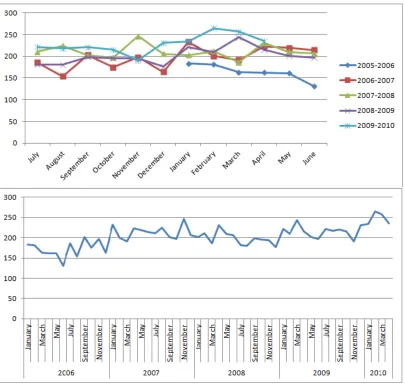
Figure 3.8: Average Procedure Duration Each Year for Procedures with CPT Code 66984 Based on 2238 Observations

cw. We use D to denote the random variable procedure duration with density function f(D), x∗ to denote the optimal estimated procedure duration, andeto denote the time length earlier than the scheduled procedure start time that all resources are ready, for example, if we only consider patients’ arrival, then it would be the amount of time the patient is required to arrive and be ready prior to their scheduled procedure start time. So the expected total idle time cost and waiting time cost would be:

total cost = ciE[(x∗−e−D)+] +cwE[(D−x∗)+] = ci

Z x∗−e

0

(x∗−e−D)f(D)dD+Cw

Z ∞

x∗

(41)

Figure 3.9: Average Procedure Duration Each Year for Procedures with CPT Code 27447 Based on 331 Observations

To find x∗ that minimizes the total cost, we take the derivative of the total cost function with respect tox∗ and set it to be zero, thusx∗ should satisfy the following equation:

ciP{D≤x∗−e}=cwP{D≥x∗} (3.2)

(42)

P{D≤x∗}= cw ci+cw

(3.3)

3.3 Length of Stay in PACU and ICU

The PACU and the ICU are important and expensive resources, and should also be considered in the OR scheduling process. The availability of the PACU and the ICU impact the effectiveness of the OR schedule. So modeling the distributions of LoS in the PACU and ICU is of interest. Based on our data analysis results, the LoS in PACU and ICU vary greatly, even for the same procedure, because it may be also very sensitive to the patient’s physical condition and other factors. Table 3.16 shows some statistics about the LoS in PACU for all orthopedics procedures and two most commonly performed procedures. You can see that there is not much difference between statistics of these three data sources. Given this insignificant difference and the limited observations, we think that it is more robust to pool the LoS of each service type together, i.e., assume that the LoS in PACU/ICU for the same service follows one distribution, and can be estimated together.

Table 3.16: Some Statistics about LoS in PACU for Orthopedics

Procedure Type No. of Observations Mean Standard Deviation CV

Orthopedics 142 144.84 135.31 0.93

27447 29 145.90 133.19 0.92

27130 22 147.95 139.02 0.94

(43)

distributions to simulate the three processes. The Norta method [Cario and Nelson, 1997] could be adopted to handle the problem.

(44)

CHAPTER 4

SIMULATION

With a better analysis of the data, a more accurate simulation model can be built to study the system as a whole. It allows us to study how good a schedule is. It also allows us to test some “what if” scenarios to determine their impact before implementation. For example, how many extra procedures will the hospital be able to perform if the standard operating hours of all ORs are extended to 10 hours? What if additional operating hours are provided during the weekends instead?

In Section 4.1, we describe the conceptual simulation model. In Section 4.2, we first use some deterministic examples taken from the historical data to verify the model; and then we show the related numerical experiments on the simulation model to study the number of replications required for desired measurement accuracy, and last we use some historical data to validate the model. Some other numerical tests are also shown in Section 5.3 with the numerical tests for generating schedules. The simulation model is used in either evaluating a schedule, or as a method for answering “what if” questions. We describe how to use the model for answering “what if” questions in Section 4.3, and describe how to evaluate schedules in Section 4.4. How to evoke the simulation in the OR Scheduling Support Information system is described in Chapter 6 with the description of the system design. Some parameters in the simulation process, e.g. total number of replications in the simulation, can be changed by the user interface as well.

First, it is necessary to define some common terms we use in the following sections:

Overtime associated with a procedure is the OR overtime associated with a procedure, which is computed as the positive difference between the finish time of the procedure and the end time of the standard operating hours of the OR/block.

Waiting time associated with a procedure is the surgical team’s waiting time associated with a procedure, which is computed as the positive difference between the actual start time and the scheduled start time of the procedure.

(45)

is computed as the positive difference between the actual start time of the next procedure and the summation of the finish time of the procedure and the turnover time after the procedure,. Workload of an OR/block is the total time that the OR/block is actually in use. It is the summation of procedure durations and turnover times.

Utilization of an OR/block is the workload of the OR/block divided by the standard oper-ating hours of the OR/block.

Total overtime of an OR/block is the summation of the overtime associated procedures performed in the OR/block.

Total waiting time of an OR/block is the summation of the waiting time associated proce-dures performed in the OR/block. It is also considered as the waiting time of all surgical teams that performed procedures in the OR/block.

Total idle time of an OR/block is the summation of the idle time associated procedures performed in the OR/block.

4.1 Conceptual Model

A Monte-Carlo simulation model is adopted here. The conceptual simulation model is shown in Figure 4.1. The objective is to replicate the hospital system described in Chapter 1 by consid-ering three resources: OR, PACU, and surgical team, and three processes: turnover, performing surgical procedure and recovering in PACU. The details are described as follows.

Workflow.A patient is sent to OR for a surgical procedure after arrival if both the OR and surgical team are available. Depending on the case requirement, he/she may be sent to a PACU bed after the procedure is done, or depart (be sent to ICU or ward, or go home directly). We do not consider the process of patients going to ICU or ward in our model because both ICU and Ward beds are not the bottleneck resources in the case we study, and they have little impact in the scheduling decision making process. After the patient leaves the OR, the turnover process begins immediately. The OR becomes available to the next patient after the turnover is finished and if it is within the regular OR operating time range. The standard operating time range (e.g. from 8:00AM to 4:00PM) defines the time range that a new patient can be brought into the OR. If the turnover is finished after the time range, the next patient cannot be brought into the OR for the next procedure, which means that the next procedure will be canceled.

(46)

Figure 4.1: Simulation Process Illustration

Input. The input to the model contains both the availability of the resources, which includes the standard operating time of the OR and the earliest available time for each surgical team of interest, and a schedule for the schedule block, which includes a list of procedures scheduled to be performed on that particular day, the CPT code for each procedure, the performing order of these procedures, the scheduled start time for each procedure, a flag indicating whether the patient needs a PACU bed after the surgical procedure, and surgical team that performs each procedure. For example, the regular operating hour of the OR is from 8:00AM to 4:00PM; all surgeons’ earliest available times are 9:00AM; a schedule with two cases (CPT code 27447 and 27130) are also given with scheduled start time 8:00AM and 1:00PM, respectively; the 27447 case starts first, it requires a PACU bed, and surgical team A performs it; the 27130 case is the second, it does not require a PACU bed, and surgical team B performs it.

(47)

and arriving 60 minutes before schedule is required, the patient arrival time would be 11:00AM.

Process Time. We adopt the data analysis results we obtain in the previous chapter to describe the time for each process: the surgical procedure duration is assumed to follow an Empirical distribution based on all the historical procedure duration data for ones with the same CPT code, and if there is no historical data for some procedure, the Empirical distribution based on all historical data for the corresponding service is used. The turnover time follows the best-fit distribution found based on the method shown in Section 3.1.3, in the case of orthopedics service in our study, the best-fit distribution for turnover time is a Uniform distribution. The LoS in PACU are generated based on an Empirical distribution dependent on the service type.

(48)

(49)

The flow chart for this main simulation model is shown in Figure 4.2.

Input. Resource availability information and a schedule are given as the input of the simulation process.

Step 1. We generate procedure durations, the LoS in PACU (if PACU bed is required) for each case, and turnover time after each procedure for all the replications.

Step 2.Initialize Replication = 1. Step 3.Initialize Procedure = 1. Step 5.Compute procedure start time.

– Procedure start time = max{ OR available time, surgical team available time, pa-tient’s arrival time};

– OR available time = max{ Previous Patient Leaving OR Time + Turnover Time after Previous Procedure, OR open time}.

Step 6. Check whether the procedure start time computed in Step 5 exceeds the OR standard operating time range. If it does not exceed the time range, which means that the patient can be brought into the OR, continue to Step 8; Otherwise, the corresponding procedure has to be canceled, go to Step 7.

Step 7. Moved the procedure index back to the previous one (i.e. the last procedure performs) for computing measurements in Step 13.

Step 8.Update Total Idle Time and Total Waiting Time of the block.

– Idle Time before = Current Procedure Start Time−Finish Time of Previous Proce-dure−Turnover Time after Previous Procedure;

– Waiting Time before =max{0, Current Procedure Scheduled Start Time−Current Procedure Start Time };

– Total Idle Time = Total Idle Time + Idle Time before;

– Total Waiting Time = Total Waiting Time + Waiting Time before. Step 9.Compute current patient leaving OR time.

– If PACU bed is required:

(50)

* Patient Leaving OR Time =max{Procedure Start Time + Procedure Duration, PACU Available Time}.

– Else:

* Patient Leaving OR Time = Procedure Start Time + Procedure Duration. Step 10. Update Total Workload.

– Total Workload = Total Workload + Current Procedure Duration + Turnover Time after Current Procedure.

Step 11.Check whether the current procedure is the last procedure in the schedule list. If it is the last procedure, which means that we have gone through all procedures in the current replication, go to Step 13; Otherwise, go to Step 12 to continue to the next procedure.

Step 12. Increment procedure index. Go to Step 5.

Step 13. Update the total idle time or the total overtime of the block.

– Idle Time after = max{ 0, Turnover Finish Time - OR Standard Operating End Time };

– Overtime =max{ 0, Turnover Finish Time - OR Standard Operating End Time}; – Total Idle Time = Total Idle Time + Idle Time after;

– Total Overtime = Total Overtime + Overtime;

– Total Number of Procedures = Total Number of Procedures + Current Procedure Index.

Step 14. The current replication is complete, and check whether the current replication counter is less than the total number of replications. If the desired number of replications have been finished, go to Step 16 to compute the statistics; otherwise, go to Step 15.

Step 15. Update the replication counter. Go back to Step 3 for the next replication. Step 16. Compute the desired statistics.

– Expected Workload = Total Workload /Number of Replications;

– Expected Utilization = Expected Workload/Length of the OR Standard Operating Time;

(51)

– Expected Total Idle Time = Total Idle Time /Number of Replications;

– Expected Total Waiting Time = Total Waiting Time /Number of Replications; – Expected Total Overtime = Total Overtime/ Number of Replications;