Detection of Denial of QoS Attacks on DiffServ Networks.

(1)

MAHADIK, VINAY ASHOK. Detection of Denial of QoS Attacks on DiffServ Networks. (Under the direction of Dr. Douglas S. Reeves.)

(2)

by

VINAY ASHOK MAHADIK

A thesis submitted to the Graduate Faculty of North Carolina State University

in partial fulfillment of the requirements for the Degree of

Master of Science

Computer Networking

Raleigh

2002

APPROVED BY:

(3)

(4)

BIOGRAPHY

Vinay A. Mahadik received his Bachelor of Engineering Degree in Electronics and Telecommunications in 2000 from the University of Mumbai (Bombay), India. Presently, he is pursuing a Master of Science degree in Computer Networking at the North Carolina

(5)

ACKNOWLEDGEMENTS

The official name for this project is ArQoS. It is a collaboration between the North Car-olina State University (Raleigh), the University of California at Davis and MCNC (RTP). This work is funded by a grant from the Defense Advanced Research Projects Agency, ad-ministered by the Air Force Rome Labs under contract F30602-99-1-0540. We gratefully acknowledge this support.

I would like to sincerely thank our co-researchers Dr. Fengmin Gong with Intruvert Networks, Dan Stevenson and Xiaoyong Wu with the Advanced Networking Research group at MCNC, and Dr. Shyhtsun Felix Wu with the University of California at Davis. Special thanks to Dr. Gong for allowing me to work on ArQoS with ANR, and to Xiaoyong, whom I worked closely with and tried hard, and failed, to compete technically with; nevertheless, it has been a highly rewarding experience.

I would also like to thank my friends Akshay Adhikari who provided significant technical help with this work, and Jim Yuill for his immensely influential and practical philosophies on information security, particularly on deception and uncertainty; I am sure these will influence my security research approach in the future.

My sincerest thanks to Dr. Douglas S. Reeves for his infinitely useful advice and guidance throughout my work; it has been a pleasure to have him as my thesis advisor. Thanks are also due to Dr. Gregory Byrd, Dr. Jon Doyle and Dr. Peng Ning for agreeing to be on my thesis research committee and providing valuable input.

(6)

List of Figures

1.1 A Simplified DiffServ Architecture . . . 2

1.2 DiffServ Classification and Conditioning/Policing at Ingress . . . 2

1.3 Differentially Serving Scheduler . . . 3

2.1 A typical DiffServ cloud between QoS customer networks . . . 11

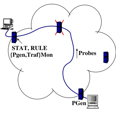
2.2 How the ArQoS components are placed about a VLL . . . 14

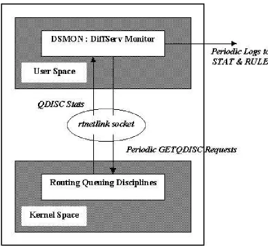
2.3 DSMon : DiffServ Aggregate-Flows Monitor . . . 15

2.4 Pgen : Probes Generation Module . . . 17

2.5 Pgen mon and Traf mon : Probe and Micro-Flow Monitor . . . 19

3.1 χ2 _{Statistical Inference Test . . . .} ₂₆

4.1 EWMA SQC chart for a Normal process . . . 36

5.1 Network Setup for Tests . . . 41

5.2 Network Topology for the Simulations . . . 44

6.1 BE Background Traffic with 1, 10 and 100 Second Time Scales. . . 49

6.2 CBR Traffic with 1, 10 and 100 Second Time Scales. . . 50

6.3 Screen capture of an Alerts Summary generated for over an hour. Shows an attack detection Red ”alert-cluster”. . . 54

6.4 Curves illustrating the tradeoff between Detection Rate (from ST P eriod) and False Positive Rate (from Ns) . . . 56

6.5 Screen capture of the long term distribution for the self-similar traffic’s byte rate statistic . . . 58

6.6 Screen capture of the Qdistributions of the self-similar background traffic’s byte rate and the jitter of BE probes . . . 59

6.7 Screen capture of the Q and long term distributions for the MPEG4 QoS flow’s byte rate statistic . . . 64

(9)

List of Tables

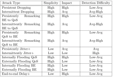
1.1 Likelihood, Impact and Difficulty-of-detection for Attacks . . . 7

6.1 NS2 Traffic Service Differentiation . . . 48

6.2 Results of EmulationTests on Anomaly Detection . . . 60

(10)

List of Symbols

α NIDES/STAT’s False Positive Rate Specification Parameter AF, BE, EF Assured Forwarding, Best Effort, Expedited Forwarding

CBS Committed Burst Size in bytes

CIR Committed Information Rate in bytes per second DiffServ Differentiated Services

DSCP Differentiated Service Code Point

EWMA Exponentially Weighted Moving Average/-based SPC Chart

FPR False Positive Rate

IDS Intrusion Detection System

ILP eriod NIDES/STAT’s Inter-Log (Sampling) Period

LCL EWMA’s Lower Control Limit

LT E EWMA’s Long Term Estimate

LT P eriod NIDES/STAT’s Long Term Profile Period

PGen Probes Generator

PgenMon Probes Monitor

Q NIDES/STAT’sQ Anomaly Measure

QoS Quality of Service

RED Random Early Dropping Congestion Avoidance Algorithm

RULE Rule-based Detection Engine

S NIDES/STAT’s Normalized Anomaly Detection Score

SLA Service-Level Agreement

SPC Statistical Process Control

STAT Statistical Anomaly Detection Engine

(11)

ST P eriod NIDES/STAT’s Short Term Profile Period

TBF Token Bucket Filter

TCA Traffic Conditioning Agreement

TrafMon Traffic Monitor

U CL EWMA’s Upper Control Limit

VLL Virtual Leased Line

(12)

Chapter 1

Introduction

As Quality of Service (QoS) capabilities are added to the Internet, our nation’s business and research infrastructure will increasingly depend on their fault tolerance and survivability. Current frameworks and protocols, such as Resource ReSerVation Proto-col (RSVP)[10] / Integrated Services (IntServ)[46] and Differentiated Services (DiffServ) [26, 3], that provide quality of service to networks are vulnerable to attacks of abuse and denial[3, 41, 10]. To date, no public reports have been made of any denial of QoS attack incidents. However, this absence of attacks on QoS is an indication of the lack of a large scale deployment of QoS networks on the Internet. Once, QoS deployments become com-monplace, the potential for such attacks to maximize damages will increase and so would an adversary’s malicious intent behind launching them. It is necessary both to make the mechanisms that provide QoS to networks, intrusion tolerant and detect any attacks on them as efficiently as possible.

This work describes a real-time, scalable denial of QoS attack detection system with a low false alarm generation rate that can be deployed to protect DiffServ based QoS domains from potential attacks. We believe our detection system is the first and the only public research attempt at detecting intrusions on network QoS.

1.1 Differentiated Services

(13)

(PHB) groups implemented on each node. The domain consists of DiffServ boundary nodes and DiffServ interior nodes.

Ingress Router Core Routers Egress Router

Classification

Conditioning {Metering, Marking, Shaping} Scheduling Scheduling Scheduling ! ! ! ! ! " " " " " # # # # # $ $ $ $ $ % % % % % & & & & & ' ' ' ' '

Figure 1.1: A Simplified DiffServ Architecture

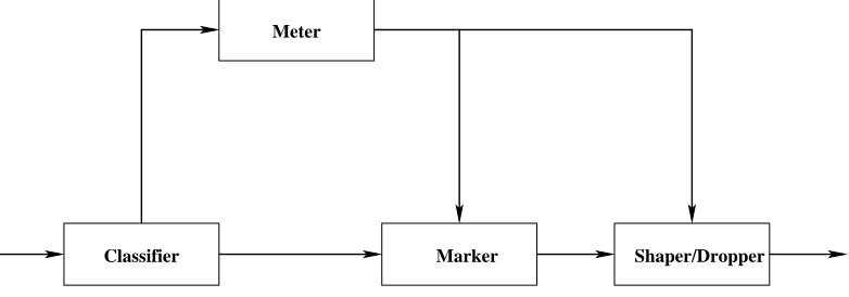
Classifier Marker Shaper/Dropper

Meter

Figure 1.2: DiffServ Classification and Conditioning/Policing at Ingress

Figure 1.1, in combination with Figures 1.2 and 1.3, illustrates the various DiffServ mechanisms in a simplified configuration (single DiffServ domain with exactly one pair of ingress and egress routers, looking at only one-way traffic from the ingress to the egress). The reader is referred to RFC 2475[3] for more complex configurations, exceptions, multi-domain environments, and definition of terms.

(14)

EF

AF

BE

Scheduler (e.g. WRR)

DiffServ−ed Flow

Figure 1.3: Differentially Serving Scheduler

mapped into a single DiffServ Code Point (DSCP), a value for a field in the IP protocol header, through a one-one or many-one mapping. Each behavior aggregate then receives a different Per-Hop Behavior (PHB), which is defined as the externally observable forwarding behavior applied at a DS-compliant node to a DiffServ behavior aggregate. The ingress boundary nodes’ key functions include traffic classification and/or traffic conditioning (also commonly referred to as policing).

• The packet classification identifies the QoS flow, that is, a subset of network traffic which may receive a differentiated service by being conditioned and/or mapped to one or more behavior aggregates within the DiffServ domain. Typical examples would be, using a DSCP mark provided by an upstream DiffServ domain, or using a source-destination IP address pair, or using the type of traffic as indicated by the service/port numbers during classification.

• Conditioning involves some combination of metering, shaping, DSCP re-marking to ensure that the traffic entering the domain conforms to the rules specified in the Traffic Conditioning Agreement (TCA). The TCA is established in accordance with the domain’s forwarding service provisioning policy for the specific customer (group). This policy is specified through a Service Level Agreement (SLA) between the ISP and the QoS Customer(s).

(15)

view. As mentioned above, this is done to make the traffic conform with the SLA/TCA specifications, so that QoS is easier to provide. Conformance with a typical SLA/TCA makes the flow statistics reasonably predictable. This incidentally, then, helps with anomaly detection applied to those statistics.

At the interior nodes, packets are simply forwarded/scheduled according to the Per-Hop Behavior (PHB) associated with their DSCPs. Thus, this architecture achieves scalability by aggregating the traffic classification state, performed by the ingress routers, into the DSCPs; the DiffServ interior nodes do not have to maintain per-flow states as is the case with, say, IntServ. In other words, in a DiffServ domain, the maintenance of per-flow states is limited to the DiffServ cloud boundary, that is, the boundary (ingress) nodes.

The DiffServ Working Group defines a DiffServ uncompliant node as any node which does not interpret the DSCP and/or does not implement the common PHBs.

DiffServ are extended across a DiffServ domain boundary by establishing a SLA between an upstream DiffServ domain and a downstream DiffServ domain, which may specify packet classification and re-marking rules and may also specify traffic profiles and actions to traffic streams which are in- or out-of-profile.

PHBs that the architecture recommends are Assured Forwarding (AF)[14], Ex-pedited Forwarding (EF)[18] and Best Effort (BE, zero priority) service classes. Briefly, an AF class has multiple subclasses with different dropping priorities marked into their DSCPs. Thus these classes receive varying levels of forwarding assurances/services from DS-compliant nodes. The intent of the EF PHB/class is to provide a service category in which suitably marked packets usually encounter short or empty queues to achieve expe-dited forwarding, that is, relatively minimal delay and jitter. Furthermore, if queues remain short relative to the buffer space available, packet loss is also kept to a minimum. A BE class provides no relatively prioritized service to packets that are marked accordingly.

1.2 DiffServ Vulnerabilities

(16)

leaves scope for attackers who can modify or use these service class code points to effect either a denial or a theft of QoS which is an expensive and critical network resource. With these attacks and other non QoS-specific ones (that do not make use of DSCPs), there is the possibility of disrupting the entire QoS provisioning infrastructure of a company, or a nation. The DiffServ Working Group designed and expect the architecture to withstand random network fluctuations; however, the architecture does not address QoS disruptions due to malicious and intelligent adversaries.

Following are the attacks we identified, all of which, we believe, can be detected or defended against by a DiffServ network in combination with our detection system. A malicious external host could flood a boundary router congesting it. A DiffServ core router itself can be compromised. It can then be made to remark, drop, delay QoS flows. It could also flood the network with extraneous traffic.

We focus only on attacks and anomalies that affect the QoS parameters typically specified in SLAs such as packet dropping rates, bit rates, end-to-end one-way or two-way delays, and jitter. For example, an EF service class SLA typically specifies low latency/delay and low jitter. An EF flow sensor then monitors attacks on delay and jitter only. Attacks that lead to information disclosure, for example, are irrelevant to QoS provisioning, and thus to this work. Potential attacks we study are as follows.

• Packet Dropping Attacks. A compromised router can be forced to drop packets em-ulating network congestion. Some QoS flows may require exceptionally high packet delivery assurances. For example, for Voice-over-IP flows, typical SLAs guarantee sub 1% packet drop rates. Network-aware flows, such as those based on the TCP protocol, may switch to lower bit rates, perceiving the packet dropping as a sign of unavoidable network congestion.

• DSCP Remarking Attacks. Remarking out-of-profile packets to lower QoS DSCP marks is normal and suggested in the standard. A malicious exploit might deceptively remark even in-profile packets to a lower QoS or could remark a lower QoS flow’s packets to higher QoS marks, thus enabling them to compete with the higher QoS flow.

(17)

heavy book keeping, schedule a QoS flow’s packets such that some are forwarded expeditiously while others are delayed. The effect is to introduce extra jitter in the QoS flow that is sensitive to it.

• Flooding. A compromised router can generate extraneous traffic from within the DiffServ network or without. Furthermore, the generated flood of traffic could be just a best-effort or no-priority traffic or a high-QoS one for greater impact.

• Increase End-to-end Delay. Network propagation times can be increased by a mali-cious router code by delaying the QoS flow’s packets with the use of kernel buffers and timers. This will be perceived by end processes as a fairly loaded or large network.

Consider the Table 1.1 which gives the simplicity, the impact and the expected difficulty of detection for each attack that we investigate.

• Simplicity, and thus the expected likelihood of an attack, is low when a significant effort or skill is required from the attacker or his/her malicious module on a compro-mised DiffServ router. For example, to be able to increase jitter and/or delay of a flow while not effecting (an easily detectable) dropping on it, the malicious code has to manage the packets within the kernel’s memory and it involves significant book-keeping; whereas, dropping packets only requires interception and a given dropping rate.

• Attacks are easier to detect (statistically) if the original profile/distribution of the QoS parameter they target is well suited for anomaly detection (strictly or weakly stationary mean etc). Jitter is thus, typically, not a good subject for this, while the bit rate for a close-to-constant bit rate flow with a low and bounded variability about the constant mean is.

1.3 QoS Intrusion Detection Challenges

(18)

Attack Type Simplicity Impact Detection Difficulty

Persistent Dropping High High Low-Avg

Intermittent Dropping High Avg Avg-High Persistently Remarking

BE to QoS

High High Low-Avg

Intermittently Remarking BE to QoS

High Avg Avg-High

Persistently Remarking QoS to BE

High High Low-Avg

Intermittently Remarking QoS to BE

High Avg Avg-High

Persistently Jitter+ Low Avg Avg

Intermittently Jitter+ Low Low High

Internally Flooding QoS High High Low-Avg Externally Flooding QoS High Low Low-Avg Internally Flooding BE High Low Low-Avg Externally Flooding BE High Low Low-Avg

End-to-end Delay+ Low High Low-Avg

Table 1.1: Likelihood, Impact and Difficulty-of-detection for Attacks

• Slow and Gradual Attacks : Statistical Intrusion Detection Systems (IDSs) are known to fail[24] when attacked over long enough periods of time that render them insensitive. Specifically for QoS, a slow enough degradation of the network QoS might be viewed by a monitor as a normal gradual increase in network congestion level and thus not flagged as an anomaly or attack.

(19)

the aggregate flow does not smooth out when measured over longer time scales. The bit rate for such an aggregate flow is therefore, not practically deterministic or pre-dictable. That is, in other words, after a sufficiently long period of observation of the traffic rate/profile, at any point, it is neither possible to accurately or approximately predict the traffic profile in the near future nor is the recent past traffic profile ap-proximately similar to the long term one observed. Whereas, an individual streaming audio or video flow will by design (encoder or compatibility with fixed-bandwidth channel issues etc), in the absence of effects like network congestion, typically tend to be either a constant bit rate flow or a low-deviation variable bit rate one. In ei-ther case, since the variability is bounded, the flow’s bit rate exhibits predictability and is a suitable subject for statistical modelling or profiling, and hence for anomaly detection.

1.4 Contribution of the Thesis

This is the first comprehensive QoS monitoring work. Intrusion Detection is an actively researched area. Statistical Anomaly Detection is a subset of this area. It focuses on attacks that do not have any easily specifiable signatures or traces that can be effectively detected or looked out for. It also aims at detecting those unknown attacks which might only appear as unexplained anomalies in the system (for example) to a Signature or Rule based IDS. This approach is both introduced and elaborated upon in Chapters 3 and 4.

QoS monitoring is a potential application area for Statistical Anomaly Detection. Our contributions to this application area are

-• We adapt and extend an existing Statistical Anomaly Detection algorithm (SRI’s NIDES algorithm) specifically for a QoS provisioning system.

• We adapt the EWMA Chart Statistical Process Control (SPC) technique for QoS monitoring. We believe this work is the first to use SPC Charts for both intrusion detection in general and QoS monitoring in particular.

• We use a signature or rule-based detection engine for use in tandem with the anomaly and process control techniques.

(20)

statistic(s) they target, and predict their likelihood of occurrence or simplicity of implementation/deployment, impact on the QoS flow in general, and the typical dif-ficulty an anomaly detection system would have in monitoring a QoS flow for such an attack.

• We create emulated and simulated DiffServ domain testbeds for study of the attacks and the detection system.

• We develop research implementations of these attacks for both the emulated and the simulated testbeds.

• We provide results of the attack detection emulation and simulation experiments we do.

• We recommend values for the detection systems’ parameters apt for QoS monitoring.

• Finally, we discuss open problems with QoS monitoring and suggest possible future research directions.

1.5 Thesis Organization

(21)

Chapter 2

QoS, Attack and Detection System

Framework

This chapter elaborates on the framework used for the attacks and the detection system. The preceding chapter introduced the attacks of interest, viz, packet dropping, DSCP remarking, increasing jitter, increasing end-to-end delay, and network flooding. The QoS flow parameters that these attacks target are the byte rate, the packet rate, the jitter, and the end-to-end delay of a QoS flow. We emulate these attacks through research im-plementations of each on an emulated DiffServ Wide-Area Network (WAN) domain. The implementation details of the attacks themselves are not described in this work for brevity. Our detection system is a combination of a Statistical Anomaly Detection system, a Statisti-cal Process Control (SPC) system (together referred to as NIDES/STAT) and a Rule-based Anomaly Detection system (RULE). The statistical systems are described in detail in the chapters 3 and 4 respectively. The rule based system, RULE, is described later in this chapter.

2.1 Motivation and Goals

In this section, we give an overview of the philosophy behind, and the business case for QoS anomaly detection.

(22)

guarantees (in the form of SLAs and TCAs) to the customer networks’ flows when they flow through the ISP’s network. An attacker could have compromised some of the ISP’s core routers and could thus attempt to disrupt the QoS flows the customer networks have subscribed for to achieve any of a myriad number of possible objectives like pure malicious thrill, reducing the reliability and thus the reputation of the ISP, or disrupting the customer networks’ businesses.

VLL

DiffServ Network Cloud

! ! " " # $ % & ' ' ' ' ' ( ( ( ( ) ) ) ) * * * * + + + + + , , , , -. . . .

Figure 2.1: A typical DiffServ cloud between QoS customer networks

(23)

also out-source the security requirements to a Managed Security Services (MSS) provider which specializes in (QoS) security administration. In this thesis, we use the termsdomain administrator orsecurity officer interchangeably to refer to the person who configures the QoS VLL (explained below) and/or our detection components monitoring it.

2.2 Framework Assumptions

Our detection system framework makes the following assumptions, which we be-lieve are reasonable.

• Use of Virtual Leased Lines : Virtual Leased Lines (VLLs) were first suggested in [27] in the context of providing Premium Service in a DiffServ domain to flows subscrib-ing for QoS. The VLLs can be achieved through traffic engineersubscrib-ing on tag-switched networks like MultiProtocol Label Switching (MPLS)[35] networks. The rationale be-hind VLLs is that most QoS parameters are highly dependent on the packet routes and the nodes involved. A dynamic route reconfiguration affects these parameters unpredictably and hence can not guarantee QoS. VLLs also assist in predicting the compromised router(s), in using IP Security Protocol (IPSec) for data integrity and/or confidentiality, and also instealth probing the network as explained later in this chap-ter. Therefore, it is reasonable to expect the QoS ISPs to use an administratively configured VLL between the two boundary nodes that connect the customer networks.

(24)

2.3 Detection System and Component Architecture

This section gives an overview of the roles of and communication/coordination between the detection system components. It then describes the components in detail.

An ISP would begin by requiring the customer networks to subscribe to the added security provisioning service. It then places the attack detection engines, NIDES/STAT (both anomaly detection and process control modules) and RULE on the VLL’s egress boundary node depending on which direction of the flow is being monitored. For example, for a streaming video flow, the egress node would connect to the client network and the ingress side would connect to the streaming video server(s). Since NIDES/STAT and RULE are designed to receive inputs over the network, they could be placed on any other accessible node on the network, but as the egress routers are trusted whereas any part of the network cloud minus its boundary is not, we recommend placing them on the same local segment as the egress router on a secure and trusted node. PGen is a probe packet generator that inserts the probe packets into the VLL that help in anomaly detection as described later in this chapter. PgenMon is the corresponding sensor that measures the parameters packet rate, byte rate, jitter and, if possible (if the boundary nodes are time-synchronized), the end-to-end delay for the probes sent by PGen. PgenMon is placed on the egress node of the VLL along with NIDES/STAT and RULE while PGen is on the ingress node. Similarly, TrafMon is a sensor that monitors normal (as against probes) data flow in the VLL for byte and packet rates (only). The placement of the various components about the VLL is as shown in the Figure 2.2.

The sensors PgenMon and TrafMon sample the QoS flow statistics periodically and send it to the NIDES/STAT and RULE attack detection engines. Our test implementations of the attacks are run as kernel modules on a core/interior node on the VLL being moni-tored. NIDES/STAT detects attacks through an elaborate statistical procedure described in the next two chapters, while RULE does a simple bounds-check based on the SLA/TCA to determine if an QoS exception has occurred that needs administrative attention. The NIDES/STAT and RULE presently log attack alerts to local files that can be parsed and viewed over secure remote channels from a central console. All the sensors and the detection engines can also be configured from user-space, so that the ISP’s domain administrator can manage the security of each VLL remotely.

(25)

-Probes STAT, RULE {Pgen,Traf}Mon PGen

Figure 2.2: How the ArQoS components are placed about a VLL

• NIDES/STAT : TheStatistical Anomaly Detection engine, accepts inputs from sen-sors on local or remote networks. NIDES/STAT modules are placed on one of the boundary routers of a VLL being monitored. If that boundary router is shared by more than one VLL, the NIDES/STAT process can be shared between them too. The following two chapters provide detailed description of this engine.

• RULE : TheRule-based Detection engine, accepts inputs from local or remote sensors. It is placed on either or both of the boundary routers of a VLL. The attack signatures we use include 1. a packet dropping rate is above a specified threshold rate for the Assured Forwarding (AF) probing traffic, or 2. EF packets are being remarked to BE (Best Effort traffic having no QoS guarantees) although the SLA/TCA specifies dropping EF packets that are delayed significantly, etc. The rules are heuristically derived, and a function of the SLA/TCA for the VLL. We recommend the use of RULE mostly as a bounds and conformity checker for the SLA. The above are only specific examples we suggest and use. Rules checking is well-understood and not further researched or discussed in this work.

(26)

Figure 2.3: DSMon : DiffServ Aggregate-Flows Monitor

(27)

viz, byte and packet counts, dropped packets count, and overlimit (or out of profile) packets count from the kernel. DSMon to kernel communication is through the Linux RTNetlink socket created by DSMon. These statistics are then periodically sent to the local or remote NIDES/STAT and RULE modules. In order that DSMon finds that an upperbound exists on the burstiness of the aggregate flow it monitors, we suggest placing the monitor only on routers that are congested or where the incident links saturate the outgoing one(s). Due to the unpredictable nature of the aggregate flow it monitors, it is found to generate an unacceptably high false positive rate. Hence, we do not use the inputs from DSMon for any of our tests in this work. We recommend its use to get an estimate of the general health of the DiffServ network in a potential future research work.

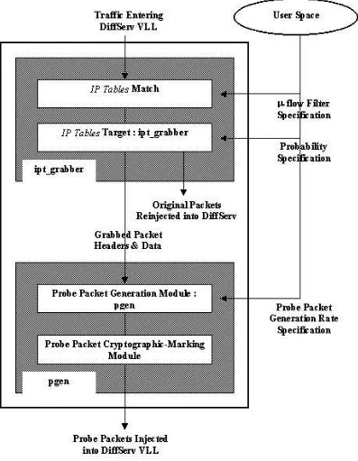
• PGen : The stealth Probe Packet Generation module is placed on the boundary routers of the VLL to be monitored. As illustrated in Figure 2.4, PGen periodically makes a copy of a random packet from the VLL inward-flow, marks the new copy with a stealth cryptographic hash and reinjects both the packets into the VLL. If a packet is not available in the VLL to be copied and reinjected, a new packet is still injected though with the contents of the packet last copied. The injection of probes is done in a soft real time manner at a low specified rate. The idea is to generate a strictly stationary flow with a fixed and known packet rate and zero jitter before entering the DiffServ cloud. The QoS parameters that are monitored for this flow then are highly predictable. Deviations from these stationary means are then a function of the DiffServ cloud. PGen also appends the hash with an encrypted sequence number for the probe packet that is necessary for jitter calculation at the egress router. It is built inside the Linux kernel as a loadable module. It operates in tandem with the iptgrabber kernel module. Once loaded, the latter copies the entire content of randomly chosen packets matching a certain filter criterion into a kernel memory buffer. It runs as a target module of a IP Tables[11] match. The match is specified through command line arguments to the iptables user space tool. We set the match to select only the VLL packets. The rate or chance of packet capture is specified through the kernel’sproc filesystem.

(28)

(29)

key between the boundary routers of the VLL and certain field(s) in the IP packets. The idea being that, then, the attacker would not be able to, with a significant level of certainty, distinguish between probe packets and the normal data packets. The use of IPSec with data encryption over the VLL clearly helps this requirement. The probes are terminated at the egress router. Interior routers simply forward packets and do not expend any processing effort on an encryption or decryption process.

Then, all attacks on the QoS of the VLL are statistically spread over both the normal data and the probe packets. We assume that such a secure probe tagging or marking method can be implemented effectively, however, we do not research this area any further in this work. In this respect, the secrecy of this mark should be considered as a single point of failure for ArQoS security for that VLL.

For jitter and delay parameters, we need monitor only the low volume probe flow. The rate of probe generation can be considered negligible compared to the rate of the VLL flow. Typical rates are 1 or 2 probe packets in a second. Large rates would have flooded the network unnecessarily while lower rates would require unacceptably longer time windows over which to generate the short term profiles, that is, a sluggish detection rate. This sluggish detection rate due to low logging sampling frequencies is a corollary to the procedure used to statistically profile and then compare the short and long term behaviors of the flow parameters, and is described both quantitatively and qualitatively in the following two chapters.

(30)

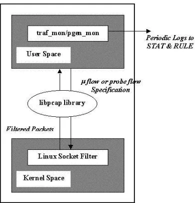
Figure 2.5: Pgen mon and Traf mon : Probe and Micro-Flow Monitor

and RULE modules to send the statistics to, the frequency of sampling the measures and of sending are all user specifiable.

(31)

(32)

Chapter 3

Statistical Anomaly Detection

3.1 The Concept

Statistical Anomaly Detection is based on the hypothesis that a system being monitored for intrusions will behave anomalously when attacked and that these anomalies can be detected. The approach was first introduced in [7]. [9] compares it with other intrusion detection approaches.

Thus far, we have used the acronym NIDES/STAT to refer to both the present sta-tistical anomaly detection engine/algorithm and the EWMA SPC Chart-based engine/technique. For this and the next chapters, and throughout the thesis, wherever they are compared against each other, we use NIDES/STAT to refer to only the anomaly detection algorithm and EWMA to refer to only the EWMA SPC Chart-based approach. The approach referred to would be apparent from the context of the discussion.

(33)

For our anomaly detection approach, NIDES/STAT, the profile referred to in long term and short term profiles is a Probability Density Function (PDF) of the monitored statistic. In view of this then, a long term profile is essentially the PDFexhibited by or observed for the statistic, in the long term period of observation of its outcomes/samples. Similarly, the short term profile is the PDF exhibited by the statistic for the recent past.

For this work, we define a statistically predictable system as one in which the long term profile of the stochastic process/system, measured by NIDES/STAT as de-fined above, does not change significantly in the time over which the short term profile is measured. As a necessary (but not sufficient) condition then, the generating moments, especially the mean and the variance, of such processes/systems do not shift significantly over the recent past as well. These are similar in spirit to the random processes that are stationary up to order 2 - the ones which have means and variances that do not vary over time. Whereas a strictly stationary process thats stationary up to order 2, severely restricts an evolution of the first and the second generating moments of the process over time, a statistically predictable system only requires (reiterating, not suffices with) that the gen-erating moments not change significantly over the recent past period over which the short term profile is calculated. Consequently, a predictable system does allow for gradual shifts in the mean and variance of the underlying base process over large multiples of the short term period. We hypothesize that for statistically predictable systems, a significant devia-tion of the short term profile from the long term profile is an anomaly. This is the radevia-tionale behind the statistical anomaly detection approach, NIDES/STAT.

3.2 Justification for using the NIDES

The Statistical Anomaly Detection approach has faced severe criticism from the intrusion detection community due mostly to its high false alarm generation rate[24]. How-ever, the effectiveness of this approach in fact depends on the nature of the subject to a large extent.

Statistical anomaly detection is, in general, well suited for monitoring subjects that have a sharply defined and restricted behavior with a substantial difference between intrusive and normal behavior. A QoS flow is an ideal candidate for such a subject and justifies the use of anomaly detection for monitoring it.

(34)

SRI’s NIDES[19] algorithm. This algorithm was originally applied to subjects which were users using a computer’s operating system and associated software utilities on it. It is impossible to accurately profile a statistically unpredictable system without making as-sumptions on the system’s behavior that are only theoretically interesting. As reasoned below, a user on a computer system and the operating system itself are unpredictable sub-jects, that can not be profiled, and are hence unsuitable for statistical anomaly detection. With that in perspective, below is a justification of why the NIDES/STAT algorithm is suitable for monitoring the network QoS.

(35)

already present in the network are protected by traffic admission control and policing at the ingress routers and also by the relatively differentiated services that flows of different priority classes experience. DiffServ SLAs and TCAs ensure that the QoS is as specified and hence predictable (in the absence of attacks). An important point to note in this context is that a failure to do so will also be considered as an anomaly and detected, irrespective of whether the network QoS was attacked externally or not. NIDES/STAT is carefully used only for QoS statistics that are predictable. Thus, for example, if a QoS flow has predictable and well bounded or defined byte rate, packet rate and end-to-end delays but unpredictable jitter, then NIDES/STAT does not monitor the jitter for such a flow. Jitter can still be monitored for that VLL by injecting probes into it. Since the probes are sourced deterministically (periodically) into the DiffServ cloud, the jitter at the egress router is a function of the DiffServ cloud only.

(36)

metering and monitoring for the SLA/TCA are not compromised. We have already justified the reasonability of this assumption in section 2.2.

• The network traffic including the probes do not have any particular distribution and instead have distributions that are specific to the network and its status. The NIDES algorithm that NIDES/STAT uses also does not assumes any specific distribution or model for the subject. The only requirement NIDES asks of the distribution is that it be fixed or slow moving, meaning the profiled process be statistically predictable. As argued before, this is a reasonable assumption for NIDES/STAT when applied to QoS flow parameters.

With this justification and motivation for the use of NIDES/STAT for QoS moni-toring in mind, we now look at the mathematical background for NIDES/STAT.

3.3 Mathematical Background of NIDES/STAT

3.3.1 The χ2 Test

The statistical anomaly detection is done by the NIDES/STAT module in com-bination with a EWMA Statistical Process Control module that monitors only highly sta-tionary processes with very low deviations (for reasons described later in this chapter). The NIDES/STAT module is treated here and the latter in the following chapter 4.

For a random variable, let E1, E2, ..., Ek represent some k arbitrarily defined,

mutually exclusive and exhaustive events associated with its outcome and let S be the sample space. Letp1,p2, ...,pk be the long-term or expected probabilities associated with

these events. That is, in N Bernoulli trials, we expect the events to occur N p1, N p2, ...,

N pk times asN becomes infinitely large. For sufficiently largeN, let Y1, Y2, ..., Yk be the

actual number of outcomes of these events in a certain experiment. Pearson[31, 15] has proved that the random variableQ defined as

Q=

k

X

i=1

(Yi−N pi)2

N pi

(3.1)

(37)

rest of the smaller ones. Rare events that do not satisfy this criterion individually may be combined so that their union may.

The pi are the long term probability distribution of the events. Let p0i = Y_Ni be

theshort term (meaning the sample size, N, is relatively small) probability distribution of the events.

Our test hypothesis, H0, is that the actual short term distribution is the same as

the expected long term distribution of the events. Its complement, H1, is that the short

term distribution differs from the long term one for at least one event. That is,

H0 :p0i =pi,∀i= 1,2, ..., k and H1 :∃i, p0i 6=pi

Since, even intuitively, Q is a measure of the anomalous difference between the actual and the expected distributions, we expect low Q values to favor H0 and high Q

values to favor H1.

(38)

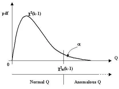
As Figure 3.1 indicates, we define α as the desired significance level of the hy-pothesis test. Also, let χ2

α(k-1) be the corresponding value of Q, that is, such that,

P rob(Q _≥ χ2

α(k −1)) = α. For an instance of Q, say qk−1, we reject the hypothesis

H0 and accept H1 ifqk₋1 ≥χ2_α(k−1).

So, with every experiment, we make N Bernoulli trials and calculate a Q based on Equation 3.1. Based on the above inequality criterion then, we determine whether, or more precisely, assume thatQand therefore the experiment was anomalous or as expected (normal).

Qualitatively, αis a sensitivity-to-variations parameter; the lower we set the value of alpha, the lesser would be the rate at which even relatively large and rare Q’s will be flagged anomalous, while the higher we set it, the higher will be rate at which even relatively lower and usualQ values will be declared anomalous.

3.3.2 χ2 Test applied to NIDES/STAT

In the context of NIDES/STAT, the random variable sampled is the measured count of a QoS parameter of the network flow being monitored. The experiment is the process of measurement or sampling of the parameter’s value. As will be seen soon, we do not sample the parameter multiple times (the N trials from above), but rather with each sample (the experiment), we use an exponentially weighted moving average process to estimate the parameter’s most recent past (short term) profile. In view of this, N takes a new formNr that’s described later in this chapter.

The QoS parameters we use presently are

• Byte Count is the number of bytes of the network flow data that have flowed in a fixed given time (from the last logging time to the present one). The rationale behind this parameter is that QoS flow sources tend to be fairly CBR or low-deviation VBR sources. As mentioned before, this is due to encoder or fixed-bandwidth channel compatibility related design issues. For example, [6] illustrates the observed CBR-like property exhibited by RealAudio sources when observed at 10s of seconds of granularity which is absent at lower (¡10s) granularities.

(39)

• End-to-end Delay is the total delay experienced by the network flow packets from the ingress to the egress of the VLL of the DiffServ cloud. Due to practical difficulties and issues with time-synchronization of the boundary nodes, we limit the use of this measure only for the tests with simulations.

• Jitter is defined as the average (of the absolute values of the) difference between the inter-arrival times of consecutive probe packet pairs arriving at the egress router of a VLL. The calculation makes use of the sequence numbers that the probe packets carry to identify the order in which the packets were actually injected into the system. For CBR sources, like the probes, using inter-arrival time jitter eliminates the need for end-to-end delay jitter. For VBR sources, to measure end-to-end delay, in general, we would need to time stamp packets at the ingress and to time synchronize the boundary routers. We focus on inter-arrival time jitter for probes only in this work.

NIDES/STAT can be extended to use other measures that matter to the SLA. NIDES/STAT is trained with the maxima and the minima of every parameter. This range is linearly divided into several equal-width (equal interval size) bins into which the count outcomes may fall. These are the events used by the χ2 Test. The number of bins is arbitrarily set at 32. Hence, any 31 events out of the total 32 events are independent. Thus we expect aχ2 Distribution for Q the maximum degrees of freedom of which are 31.

Sections 3.3.3 and 3.3.4 detail how the long term and the short term distributions of the counts are obtained.

NIDES/STAT algorithm defines a variable S to normalize the values of Q from different measures and/or flows so that they may be compared against each other for alarm intensities. This is done such thatS has a half-normal probability distribution satisfying

P rob(S²[s,_∞)) = P rob(Q > q) 2 That is,

S= Φ−1(1−P rob(Q > q)

2 ) (3.2)

(40)

3.3.3 Obtaining Long Term Profile pi

To establish the long term distribution for a measure, the detection system is first placed on the QoS domain when it has been absolutely isolated from any malicious attacks on its QoS flows (for example, when the SLAs are met and the QoS on manual inspection is as expected). NIDES/STAT is then trained with the normal (that is, unattacked) QoS flow statistics. Once it learns these training measures, it has a normal profile against which to compare a recent past short term profile for anomaly detection. The phases that NIDES/STAT goes through while building a long term normal profile are

-1. Count Training : where NIDES/STAT learns the count maxima, minima, mean and the standard deviation over a specified, sufficiently large, number of training measures. The maxima and the minima help in the linear equi-width binning used by the χ2

Test.

2. Long Term Training : At the end of a set number of long-term training measures, NIDES/STAT initializes the pi and the p0i equal simply to the bin frequencies as

pi=p0i=

CurrentCounti

CurrentT otal (3.3)

where CurrentCounti is the current number of ith-bin events and CurrentT otal is

the current total number of events from all the bins.

These are the initial long term and short term distributions.

3. Normal/Update Phase : After every preset Long Term Update Period, NIDES/STAT learns about any changes to the long term distribution itself. By using exponentially weighted moving averages, the older components in the average get exponentially de-creasing significance with every update. This is important since the flow parameters, though typically approximately stationary in a QoS network, may shift in mean over the long update period and this shift needs to be accounted for to avoid false positives. This is done as

(41)

and

pi=

b_×pi×LastW T otal+CurrentCounti

W T otal (3.6)

Here,bis defined as the weight decay rate at which, at the end of a presetLT P eriod period (long term profiling period) of time, the present estimates ofCurrentCounti

and CurrentT otal have just a 10% weight. Typically, LT P eriod is about 4 hours (as justified in chapter 6). Clearly, equation (3.6) then gives the required long term frequencies pi as the ratio of the EWMA of the current bin count to the EWMA of

the current total count. Further, only the most recent LT P eriodperiod has a (90%) significance to the long term profile.

3.3.4 Obtaining Short Term Profile p0i

Unlike the long term frequencies pi, the short term ones are updated with every

count as

p0_i =r×p0_i+ 1−r (3.7)

and

p0

j =r×p0j,∀j 6=i (3.8)

where i is the bin in which the present count falls. r is the decay rate, defined in NIDES/STAT as the rate at which the current short term bin frequency estimate has a weight of 1% at the end of a ST P eriod period (short term estimation period) of time. ST P eriod is about 15 minutes (as justified in chapter 6). The 1₋r in the equation (3.7) satisfies P

p0

i = 1 and also serves as the weight for the present count of 1 for the bin to

which the present measure belongs. Further, only the most recent ST P eriod period has a (99%) significance to the short term profile.

3.3.5 Generate Q Distribution

The calculation of the Q measure in NIDES/STAT is based on but a slightly modified version of Equation 3.1. Since the short term profilep0

i are calculated through an

(42)

to build the short term profile. We define Nr as the effective sample size based on the

EWMA process given by

Nr= 1 +r+r2+r3+...≈

1

1₋r (3.9)

which makes Equation 3.1 as

Q=

32

X

i=1

(p0

i−pi)2

pi

Nr

(3.10)

NIDES/STAT maintains along term Q distribution curve, against which each new

short term Q is compared to calculate the anomaly scoreS. The long termQ distribution generation is very similar to the long term frequency pi distribution generation. The

pro-cedure parallels the one in section 3.3.3, where equations (3.3) through (3.6) now become

-at the end of a specified long term training Qmeasures, we set

Qi=

CurrentQCounti

CurrentQT otal (3.11)

where we arbitrarily use a 32 bin equi-width partitioning, CurrentQCounti is the

current number of ith_-bin _{Q events} _and _{CurrentQT otal} _{is the current total number of} _Q events from all the bins.

Further, in the update/normal phase, after every long term update Q measures, we use

LastW QT otal=W QT otal (3.12) W QT otal=b_×LastW QT otal+CurrentQT otal (3.13) and

Qi =

b×Qi×LastW QT otal+CurrentQCounti

W QT otal (3.14)

to get the long term Q distribution.

3.3.6 Calculate Anomaly Score and Alert Level

(43)

large Qs that are consequently rare. This means both that, 1. in the absence of attacks, the False Alarms or False Positives are generated only rarely (low FPR), while 2. in the presence of attacks, only severe ones that generate exceptionally high Qs will be detected (low detection rate). αs are then set to strike a tradeoff between the required false positive and detection rates. Multiple αs can be used to classify different levels of attacks in terms of severity and likelihood.

Equation (3.2) gives the degree of anomaly associated with a new or short term generated value of Q, say q. This S score also determines the level of alert based on the following categories

-• Red Alarm Level - S falls in a range that corresponds to a Q tail probability of α= 0.001. This means thatQ’s andS’s chances of having such high a value are 1 in a 1000. (High severity, Low likelihood)

• Yellow Alarm Level - S falls in a range that corresponds to a Q tail probability of α= 0.01 and outside the Red Alarm Level range. Then,Q’s andS’s chances of falling in this tail area are roughly 1 in a 100. (Medium severity, Medium likelihood)

• NormalAlarm Level - For all values ofS below the Yellow Alarm Level, we generate a Normal Alarm that signifies an absence of attacks. (Normal level, Usual)

If after an attack is detected, it is not eliminated within the LT P eriod period of time, NIDES/STAT learns this anomalous behavior as normal and eventually stops generating the attack alerts.

Certain parameters such as the drop rate associated with an AF probe flow in an uncongested network may be highly stationary with zero or very low deviations. For such parameters, the long term frequency distributionpi does not satisfy the N pi >5 rule

for all expect possibly one or two bins. The χ2 test does not gives good results for such parameters. NIDES/STAT does make an attempt to aggregate rare bins which do not satisfy this criterion into a single event that does (due to increased bin frequency). We find, however, that whenever the number ofQi components calculated satisfying the above

(44)

for finding the anomaly score. When it exceeds or equals 3, we switch back to theχ2 _mode.

In simpler words, for QoS statistics with extremely low-deviation long term distributions, which do pose this problem, we switch to EWMA Control Chart mode to generate anomaly scores.

(45)

Chapter 4

EWMA Statistical Process Control

The Exponentially Weighted Moving Average (EWMA) Control Chart is a popular Statistical Process Control technique used in the manufacturing industry for product quality control. In this, a probability distribution curve for a statistic gives the rarity of occurrence of a particular instance of it. Outcomes that are rarer than a certain predefined threshold level are considered as anomalies. As explained, the NIDES/STAT algorithm is not suitable for a highly stationary measure with very low deviations, and it is for only such measures that we use the EWMA Control Charts to detect intrusions.

For example, a QoS customer network could be sourcing a relatively unpredictable VBR flow with mean packet and byte rates shifting swiftly over time, and could reserve a QoS bandwidth to accommodate even the highest rates it generates (over provision). The flow itself might be very sensitive to packet dropping and would reserve an AF (Assured Forwarding with low drop precedence) QoS class from the DiffServ ISP for that. The ISP would then use probes to monitor the packet rates, since the flow’s corresponding statistic is not suited for anomaly detection. Due to the use of AF class and over provisioning though, the flow could receive exceptionally low packet drop rates. In this case then, the statistic produces an exceptionally stationary (since probes are inserted into the VLL at a fixed soft real-time rate) distribution with a deviation too low for NIDES/STAT to profile or handle using theχ2 test. However, due exactly to this exceptionally high predictability, the statistic is well suited for the EWMA Statistical Process Control technique.

(46)

arbitrary subjects will lead to excessive false alarms.

4.1 Statistical Process/Quality Control

Shewhart[38, 39, 37] first suggested the use of Control Charts in the manufacturing industry to determine whether a manufacturing process or the quality of a manufactured product is in statistical control. The EWMA Control Charts, an extension of the Shewhart Control Charts, are due to Roberts[34].

In EWMA Control Charts, the general idea is to plot the statistic²k given as

²k=λxk+ (1−λ)²k−1 (4.1)

Here, a subgroup of samples consists ofnindependent readings of the parameter of interest (from n different manufactured products at any instant of time). Samples are taken at regular intervals in time. Then, xk is the average of the kth subgroup sample. λ is the

weight given to this subgroup average. ²k is the estimator for this subgroup average at kth

sample. The iterations begin with ²0 =x. x is the (estimate of the) actual process mean,

while ˆσ is the (estimate of the) actual process standard deviation.

Ifλ_≥0.02, as is typical, oncek_≥5, the process Control Limits can be defined as

x±3√σˆ

n s

λ

2−λ (4.2)

Let U CLdenote the upper control limit andLCL denote the lower control limit, ST E denote the short term estimate andLT E denote the long term estimate. For a base process that is Normally distributed, theST E estimator then falls outside the control limits less than 1% of times.

Ignoring the first few estimates then, when the iterations stabilize, we consider any estimate outside the control limits as an anomaly. The cause of the anomaly is then looked for and if possible eliminated. If the fault(s) is not corrected, the control chart eventually accepts it as an internal agent.

(47)

In case of samples that do not involve subgroups, that is, where n= 1, the equa-tions (4.1) and (4.2) become

²k=λxk+ (1−λ)²k−1 (4.3)

and

x±3σ s

λ

2−λ (4.4)

where we begin with ²0 =x.

It is important to note that theX chart (based on subgrouping) is more sensitive in detecting mean shifts than the X chart[36] (based on individual measures). Hence, wherever possible the X chart should be preferred.

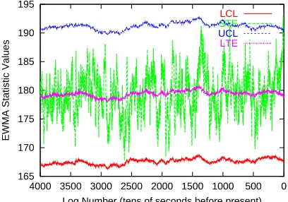
The value of the EWMA weight parameter λ is chosen as a tradeoff between the required sensitivity of the chart towards fault detection and the false positive rate statistically inherent in the method. A low λ favors a low false positive rate, whereas a large value favors high sensitivity. Typically, in industrial process control, it is set at 0.3. Figure 4.1 shows an EWMA SPC Chart for a statistic with a Normal distribution. It is interesting to note how closely the Control Limits LCL and U CL follow the short term estimate ST E while still allowing enough variability to it; out of the 4000 samples shown, only 2 generate process out-of-control alerts by falling beyond the control limits.

165 170 175 180 185 190 195

0 500 1000 1500 2000 2500 3000 3500 4000

EWMA Statistic Values

Log Number (tens of seconds before present)

LCL

STE

UCL

LTE

(48)

4.2 Application to Network Flows

In ArQoS, we consider the QoS flows/flow-statistics as quality controlled processes where the quality parameters of interest are the bit rates, packet drop rates, end-to-end one-way or two-one-way delays, and jitter of the flows.

A significant difference between the requirements of NIDES/STAT and EWMA is that NIDES/STAT requires a suitable subject statistic to have an approximately stationary long term distribution (all generating moments be approximately stationary), while EWMA requires only that the first generating moment, that is the mean, be approximately station-ary (and that the variance be low). Thus, a subject statistic suitable for NIDES/STAT is suitable for EWMA if it has a low variance.

In statistical process control, the EWMA control chart is used to detect small shifts in the mean of a process to indicate an out-of-control condition. In contrast, in ArQoS, we monitor flow processes that are only required to be weakly stationary, and hence have to allow for a gradual shift in their means over sufficiently long periods of time. However, a swift shift will be detected as an anomaly and flagged.

In view of the above, an actual process mean x, which we represent as LT E, is found as an exponentially weighted moving average as

LT Ek = (1−rLT)LT Ek−1+rLTxk (4.5)

where the decay parameterrLT makesLT E significant only for the past LT P eriodperiod

in time, just as with NIDES/STAT. The flow processes are chosen such that the mean does not shift significantly over this period of time. Any small shift is reflected as a shift inLT E.

Similarly, the long term count square,LT CntSq is found as

LT CntSqk = (1−rLT)LT CntSqk−1+rLTx2k (4.6)

and the long term standard deviation, ˆσ orLT StdDev is found as

LT StdDev=qLT CntSq₋LT E2 _(4.7)

The EWMA statistic²k, which we represent by our short term estimate parameter

ST Ek, is given by

(49)

where the decay rateris the same as the short term decay parameter used in NIDES/STAT. The ST E estimate has ST P eriodas the moving window of significance.

Then, the equation (4.2) gives the EWMA control limits as

LT E_±3LT StdDev√

n s

1₋r

1 +r (4.9)

wherenequals 1 for byte and packet counts, but is greater than 1 for parameters like jitter and end-to-end delay measures that are averaged over several packets.

ST Ek, LT Ek, LT CntSqk and the control limits U CLk and LCLk are calculated

for every received measure and an alarm is raised wheneverST Ekfalls beyond either of the

control limits. The EWMA control chart mode generates only Normal and Red Alarms. Although the QoS parameters of interest to us are strictly not Normally dis-tributed, nevertheless, our results indicate that the fairly stationary and low-deviation parameters we study do fall beyond the control limits only under anomalous conditions, that is, when under attack.

(50)

Chapter 5

Experiments with Attacks and

Detection

This chapter describes our experiments with the attacks and the detection system. We run two sets of experiments. One set involves an actual emulation of the DiffServ domain on a network testbed, with kernel and user space modules to generate best-effort and QoS flows, to sample QoS flow parameters, to effect the attacks, etc. The second set of experiments involves a thorough validation of the emulation tests using a network simulator to simulate the DiffServ domain, the various background and QoS flows, the attacks etc.

Due to implementation issues, we test almost the same set of attacks on both the simulation and the emulation experiments, except that with the simulations, we do not test for jitter attacks and with the emulation, we do not test for end-to-end delay attacks, and intermittent/bursty attacks. It is important to note that detection of attacks on end-to-end delay requires that the boundary routers be time-synchronized with each other, which is a fairly significant challenge. Any such implementation could have other security weaknesses like attacks on packets containing time synchronization information. We make no attempt to time-synchronize the boundary nodes in our emulation tests and thereby do not test for this particular attack in those.

(51)

The results and observations from these tests are summarized in the following chapter.

5.1 Tests to Validate Algorithms

To verify the correctness of the NIDES/STAT and the EWMA Control Chart algorithms, we use simulated normal network traffic and simulated attacks. With an in-dependent computer code (without any consideration about network topologies or effects thereof), we generate independent values for a random variable that has an arbitrary but stationary distribution (fixed mean and variance). This random variable represents any of the various QoS parameters we intend to monitor in practice. Example distributions we use include Normal, Uniform, and other bell-shaped arbitrary distributions with known means and variances that are kept fixed. These series of random variable outcomes or values then represent the normal, that is, unattacked, QoS parameter values. The NIDES/STAT, and EWMA Charts are trained with these values over a significant sample size to represent the long term period. Then, 1. the long term distribution generated by NIDES/STAT should match (at least approximately) the (equi-width binning distribution of the) original distribution of the statistic (Normal, Uniform etc). This validates the binning and EWMA estimation process used by NIDES/STAT. 2. TheQdistribution generated should approx-imately follow a χ2 distribution with k−1 degrees of freedom (from Equation 3.1), where kis determined from the original distribution’s equi-width binning and finding the number of bins that satisfy the rule-of-thumb N pi ≥5 including the rare-bins groups, if any. This

(52)

5.2 DiffServ Domain and Attacks : Emulation Experiments

5.2.1 DiffServ Network Topology Setup

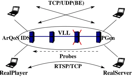
VLL RealPlayer RTSP/TCP Probes TCP/UDP(BE) PGen ArQoS IDS RealServer ! ! ! !

Figure 5.1: Network Setup for Tests

Figure 5.1 shows a condensed topology for our isolated DiffServ capable network testbed. All the routers we use are Linux kernels configured with DiffServ capabilities. For this, we use the traffic conditioning configuration utility tc that comes with iproute2[22] to configure the queueing disciplines, classes, filters and policers attached to the kernel network devices.

5.2.2 QoS-Application Traffic Setup

We setup a VLL between an ingress and an egress router. It is setup using only IP address based routing entries and DSCP based service class mappings. The VLL, sourced and sinked by a RealVideo client-server pair as shown, carries an audio-video stream that uses Real Time Streaming Protocol (RTSP) for real-time signalling, and either EF or AF (in separate tests) as the DiffServ class type for minimal delay or minimal drop rates in forwarding.

5.2.3 Background Traffic Setup

(53)

for-warding services in a moderately or heavily flooded network. Further, it is more interesting to attempt to distinguish effects on the QoS due to attacks from those due to random fluc-tuations in the background traffic. The combination of the Poisson and the HTTP models attempts to capture the burstiness (due to the HTTP model), and the randomness (due to both models) typical to the aggregate Internet traffic. We do acknowledge that this model is not entirely representative of the Internet traffic, and use a much better traffic model with the simulation experiments. To emulate a Wide Area Network (WAN), we introduce end-to-end delays and jitter in each of the routers using NISTNet[5]. We use round-trip delays with means of the order of tens of milliseconds and standard deviations of the order of a few milliseconds to emulate a moderate sized DiffServ WAN with low congestion.

5.2.4 Sensors Setup

Probes are generated at the ingress side of the video (data) flow and the PgenMon and TrafMon sensors, along with the detection engine components are placed on the egress router. We configure the video stream server to stream a Variable Bit Rate traffic (VBR) with a fixed mean rate and low deviation within the congestion that the VLL normally experiences. PgenMon monitors the jitter and the packet rate of the probes, whereas TrafMon monitors the bit rate of the video streaming (one-way) flow.

5.2.5 Attacks Setup

For the attacking agents, we again use NISTNet to significantly increase the end-to-end delays and the jitter in the QoS flows. (We test for end-end-to-end delay attacks only in the simulation experiments, and for the jitter attacks only in the emulation experiments.) We also use Linux kernel modules, we call ipt drop and ipt setTOS, as the packet dropping and packet remarking modules respectively. These are based on the IPTables’[11] packet capturing and mangling framework. The modules are written as IPTables’ kernel extensions to be called whenever a predefined filter independently captures a packet.

Thus, based on a specified filter, a selected flow can be subjected to any combi-nation of packet dropping, packet DSCP-field remarking, and introducing extra jitter and end-to-end delay variation attacks. The attack intensities are user configurable.

(54)

with the SLA. Then the individual attacks are launched to check the detection capabilities of the modules. It is important to note that the attacks can not differentiate between the probe and the video flow in the VLL.

Thus we monitor the VLL’s QoS amidst a moderate background traffic and occa-sional attacks.

5.3 DiffServ Domain and Attacks : NS2 Simulation

Experi-ments

The current version of the Network Simulator, version 2, (NS2)[43] at the time of this work has built-in DiffServ support. We use NS2 simulations extensively in our work. First, we use these to validate the results obtained from the DiffServ domain and Attacks emulation experiments. Second, and more importantly, we use these to simulate the certain other attacks not tested for in the emulation tests; namely, the attacks on the end-to-end delay and intermittent or bursty attacks.

The NS2 script used to simulate the DiffServ domain and the attacks can be found in the appendix A.

5.3.1 DiffServ Network Topology Setup

(55)

16 34 15 33 14 32 13 31 12 29 30 11 28 10 9 27 45 8 26 44 7 25 43 6 24 42 5 Sink 23 41 4 22 39 40 3 Attacking-Router 21 38 2 19 20 37 1 QoS-Customer 18 36 0 17 35

Figure 5.2: Network Topology for the Simulations

(56)

served longer in the round robin scheduling due to its greater weight, the queuing delay for that queue is reduced as well. In this way, by modifying the WRR and RED parameters of the queues in the topology, a differentiated service is provided to the QoS flow.

5.3.2 QoS-Application Traffic Setup

Node 1 represents the QoS customer that is sourcing 250kbps of either a CBR/UDP flow or a MPEG4/UDP streaming video. The former is an in-built NS2 traffic generator with an optional dither parameter that we do use. The latter captures a more realistic video streaming source and is achieved by using a NS2 trace captured and contributed by George Kinal with Femme Comp, Inc. The reader can find more information about this trace in the appendix B.

5.3.3 Background Traffic Setup

One significant difference from the emulated network, where the simulation scores is that with the latter, we use a self-similar[23, 29] BE background traffic. It is instructive to observe the behavior of a QoS flow such as a AF or EF CBR or streaming MPEG4 (say) flow when subject to the restricted influence of a self similar background traffic. Whereas, with the emulation tests, we use Poisson and empirical HTTP-modelled traffic, the combination of which is not a valid network traffic model; with the simulation tests we do not limit the validity of our tests by making simplifying assumptions on the background traffic on the network.

Each of the 40 nodes, 6 through 45, is a Pareto ON/OFF traffic source. The aggregate 4Mbps flow sourced through node 0 into the node 2 is then approximately self similar based on parameters mostly used from [21].

5.3.4 Sensors Setup

All flows are sinked in the node 5 which also has NS2 LossMonitor agents attached to monitor the packet rate and byte rate statistics of the BE background self-similar traffic and the QoS flow separately.

(57)

5.3.5 Attacks Setup

Node 3 is the compromised node that is maliciously disrupting the QoS of the flow being monitored. We use a simple procedure to effect packet dropping, and delaying attacks. For these, we simply change, at run-time, the WRR and RED parameters for the individual flows. Remarking attacks are effected by using a TBF on node 3 with a corresponding addPolicerEntry entry that gives the remarking from and to DSCP values in the specified direction. Flooding is effected simply by attaching traffic generators to the compromised node in the NS2 script.

Reiterating, the simulations help in studying the sensitivity (lowest intensities of attacks of each type that are detected) of the detection system, measuring the false alarm generation rate, and to compare the performance of the three detection approaches (NIDES/STAT, EWMA and RULE) in a fairly controlled environment. We also find the simulations immensely useful for empirical selection of the algorithm parameters.