DEMERS, ALIXANDRA. Determining Path Flows in Networks: Quantifying the Tradeoff between Observability and Inference. (Under the direction of George Fisher List.)
volume observations are also necessary – AVI or AVL data are insufficient. Considering these results, all network analyses are critically dependent upon good utilization coefficient estimates to obtain reasonable flows which, in-turn, are essential for decision-makers. This is true whether you are attempting to estimate OD flows or PUCs (say as a modeler), desiring to make good capacity investment decisions, or trying to make real-time network flow management decisions. In all cases, good quality PUCs are necessary; reliance on link flow observations would require heroic inference assumptions so AVI and/or AVL data are better choices for PUC prediction. Within this dissertation are four components to support this research endeavor and the conclusions drawn. First is a discussion of the theoretical constructs involved in the path utilization rate estimation process. Second, a methodology for estimating PUCs is presented. Third, numerical tests of the methodology are conducted on several hypothetical networks. Fourth, throughout this research three data conditions were examined to test the methodology's predictions – error-free data, stochasticity in
by
Alixandra Demers
A dissertation submitted to the Graduate Faculty of North Carolina State University
in partial fulfillment of the requirements for the Degree of
Doctor of Philosophy
Civil Engineering
Raleigh, North Carolina 2008
APPROVED BY:
Yahya Fathi Nagui Rouphail
William A. Wallace
(Rensselaer Polytechnic Institute)
Billy M. Williams
George F. List
ii BIOGRAPHY
Stuyvesant High School, New York, New York Rensselaer Polytechnic Institute, Troy, New York The University of Texas at Austin, Austin, Texas
Several years of transportation planning and engineering consulting work, primarily in Massachusetts.
Transportation Scholar at Gateway National Recreation Area – Jamaica Bay Unit
iii ACKNOWLEDGEMENTS
• Thanks to my Parental Units for their strong moral support, management acumen, and good senses of humor. Plus, thanks Dad for ensuring through your editing and explaining and my practicing that I learned how to write well, form a good argument, and properly use semi-colons – years ago!
• Thanks to my sister Christina for being great to talk to, fun to hang out with, and a great source of support.
• Thanks to Supriya for always working crazier hours at her job than I ever found a way to do and for still finding time to share long laughs and ideas over the phone – no matter what states or countries we each were in over the years.
• Thanks to my Grandpa for his huge hugs and my Grandma for hours of puzzle-solving.
• Thanks to Lydia for being a constant throughout my PhD program. I wish you the best on your journey.
iv TABLE OF CONTENTS
LIST OF TABLES ...VII
LIST OF FIGURES... VIII
LIST OF ABBREVIATIONS ... XI
LIST OF SYMBOLS... XIII
1 INTRODUCTION ...1
1.1 FRAMING THE QUESTION _______________________________________________ 4 1.2 RESEARCH OBJECTIVES _______________________________________________ 11 1.3 MOTIVATION & RESEARCH VALUE______________________________________ 11 1.4 PAPER ORGANIZATION________________________________________________ 13 2 LITERATURE REVIEW...14
2.1 INTRODUCTION______________________________________________________ 14 2.2 EXAMINING RELEVANT LITERATURE ____________________________________ 17 2.2.1 Data...17
2.2.2 Choice Behavior ...19
2.2.3 Flow Estimation ...21
2.2.4 Traffic Assignment ...24 2.3 SUMMARIZING PRIOR EFFORTS, RECOGNIZING GAPS IN CURRENT KNOWLEDGE_ 26
2.4 ANTICIPATED CONTRIBUTIONS _________________________________________ 31 v i i
v i i i
x i
v
3 METHODOLOGY ...33
3.1 PROBLEM FUNCTIONAL SPECIFICATION __________________________________ 35 3.2 THE MODEL________________________________________________________ 37 3.2.1 Notation ...37
3.2.2 Mathematical Program – First Variation (MP1) ...37
3.2.3 General Description...37
3.2.4 Objective Function ...41
3.2.5 Implications of the Model...42
3.2.6 Important Cases & Their Implications ...52
3.3 POTENTIAL PERFORMANCE MEASURES___________________________________ 56 3.3.1 Coefficient of Variation (CV) ...57
3.3.2 Sum of Absolute Errors ...57
3.3.3 Prediction Accuracy of Path Utilization Coefficients ...62
3.3.4 Root Mean Square Error ...66
3.3.5 Data Envelopment Analysis ...68
3.4 ANALYTIC TOOLS____________________________________________________ 69 4 EXPERIMENT DESIGN ...71
4.1 RANDOM PROBLEM GENERATION _______________________________________ 73 4.1.1 Physical Network ...73
4.1.2 Traffic on the Network. ...78
4.1.3 Instrumentation & Traffic Realizations ...82
4.1.4 Example Realization...84
4.2 OPTIMIZATION & OUTPUT_____________________________________________ 86 4.3 ANALYSIS___________________________________________________________ 86 5 NUMERICAL TESTS ...89
vi 5.2 EXPLORING THE RESULTS _____________________________________________ 96
5.2.1 Zero Sensor Case...96
5.2.2 Effect of Sensor Coverage, Quality, and Type ...98
5.2.3 Impact of the Origin-Destination Matrix ...119
5.2.4 Results Summary...140
5.2.5 Early Conclusions...142
6 CONCLUSIONS AND FUTURE WORK ...144
6.1 CONCLUSIONS______________________________________________________ 144 6.1.1 Motivations Revisited ...144
6.1.2 Contributions to Knowledge ...145
6.1.3 Results in Perspective ...146
6.2 FUTURE WORK _____________________________________________________ 149 6.2.1 Simple Networks ...149
6.2.2 Validation & Robustness of Technique ...152
6.2.3 More Complex Networks...153
6.2.4 Discovering Paths within a Compromised Network ...153
6.3 WRAP-UP__________________________________________________________ 154 7 REFERENCES ...155
APPENDIX ...163
8 APPENDIX A: MATH PROGRAM IN LINGO CODE...164
9 APPENDIX B: VBA CODE SUBROUTINE SUMMARY ...166
vii LIST OF TABLES
TABLE 1.1 SENSOR ATTRIBUTES RELATED TO PATH RECONSTRUCTION...9
TABLE 3.1 COMPARISON OF SAE AND SSE...57
TABLE 4.1 GRAPH THEORETIC TRANSPORT NETWORK DESCRIPTORS...73
TABLE 4.2 EXAMPLE REALIZATION OF A NETWORK...85
TABLE 4.3 SAMPLE SCENARIOS...87
TABLE 5.1 EXPECTATIONS OF SOME BASE CASES...91
TABLE 5.2 SUMMARY STATISTICS OF THE BASE CASES...92
TABLE 5.3 SUMMARY STATISTICS FOR ZERO SENSOR CASE...96
TABLE 5.4 TWO-WAY ANOVA TABLE OF ρ(xp, xˆp)FOR THE X?Q?, D100Q100 SET OF CASES... 104
TABLE 5.5 RESULTS SUMMARY WITH D100Q100... 109
TABLE 5.6 RESULTS SUMMARY WITH D20Q20... 120
viii LIST OF FIGURES
FIGURE 1.1 SIMPLE NETWORK WITH ONE OD PAIR...4
FIGURE 1.2 DIFFERENT INSTRUMENTATIONS OF NETWORK...6
FIGURE 2.1 TRADEOFF BETWEEN DATA AND INFERENCE...14
FIGURE 2.2 POTENTIAL EFFECT ON PATH DISCERNMENT OF PARTIAL AVL COVERAGE...16
FIGURE 2.3 PATH FLOW BUILDING BLOCKS...17
FIGURE 2.4 CATEGORIZING PATHS BASED ON THEIR DIRECTNESS...22
FIGURE 2.5 THE TRADEOFF BETWEEN INFERENCE AND OBSERVABILITY...28
FIGURE 2.6 POTENTIAL INFERENCE VS. OBSERVABILITY GRAPHS FOR DIFFERENT SENSOR TYPES...30
FIGURE 3.1 FLOW OF DATA IN THE PROBLEM...38
FIGURE 3.2 SHIFTED MEANS OF DOD MATRIX...47
FIGURE 3.3 POTENTIAL IMPACT OF AN INACCURATE OD MATRIX ON LINK FLOWS...48
FIGURE 3.4 THE EFFECT OF SCREEN LINE CHOICE ON COUNTING PATH FLOWS...49
FIGURE 3.5 SCREEN LINES AND ISOBARS...50
FIGURE 3.6 INFERENCE AND OBSERVABILITY COMBINATIONS FOR THREE VARIABLES...53
FIGURE 3.7 FLOW DIFFERENCES ON ARC 1 FOR AN EXAMPLE CASE...59
FIGURE 3.8 FLOW DIFFERENCES ON ALL LINKS FOR ALL SIMULATION RUNS OF A SET...60
FIGURE 3.9 LINK UTILIZATION COEFFICIENTS FOR AN EXAMPLE CASE...61
FIGURE 3.10 UNWEIGHTED PUC PREDICTION ACCURACY – 2 VARIATIONS...62
FIGURE 3.11 WEIGHTED PUC PREDICTION ACCURACY...63
ix
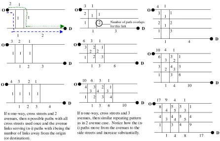
FIGURE 3.13 EXAMINING PATH IMPLICATIONS FOR A ONE-WAY MANHATTAN METRIC...65
FIGURE 3.14 RMSELUC VS. QUANTITY OF INSTRUMENTATION – 3 CASES...67
FIGURE 4.1 EXPERIMENT DESIGN...72
FIGURE 4.2 POSSIBLE SENSOR INSTRUMENTATION SCENARIOS...83
FIGURE 5.1 SAMPLE NETWORKS...90
FIGURE 5.2 OBJECTIVE FUNCTION VALUES VERSUS CORRELATIONS FOR BASE CASES...94
FIGURE 5.3 SAMPLE RESULTS FOR A REPRESENTATIVE NETWORK (NETWORK 10 WITH 25 OD FLOW REALIZATIONS) ...95
FIGURE 5.4 OBJECTIVE FUNCTION VALUES FOR THE X?Q100 (TOP) AND X100Q? (BOTTOM) CASES (BOTH WITH D100Q100) ... 105
FIGURE 5.5 PEARSON CORRELATION VALUES FOR THE X?Q100 (TOP) AND X100Q? (BOTTOM) CASES (BOTH WITH D100Q100) ... 106
FIGURE 5.6 RELATIONSHIPS BETWEEN OBJECTIVE FUNCTION AND CORRELATIONS AS PATH COVERAGE INCREASES (D100Q100 FOR ALL CASES)... 107
FIGURE 5.7 RELATIONSHIPS BETWEEN OBJECTIVE FUNCTION AND CORRELATIONS AS PUC QUALITY DECREASES (D100Q100 FOR ALL CASES)... 108
FIGURE 5.8 OBJECTIVE FUNCTION VALUE VERSUS CASES... 115
FIGURE 5.9 CORRELATION (X, XHAT) VERSUS CASES... 116
FIGURE 5.10 CORRELATION (Y, YHAT) VERSUS CASES... 117
FIGURE 5.11 CORRELATION (V, VHAT) VERSUS CASES... 118
x FIGURE 5.13 OBJECTIVE FUNCTION VALUES FOR D100Q100 VERSUS D20Q20 CASES WITH
X100Q?... 128 FIGURE 5.14 RELATIONSHIPS BETWEEN OBJECTIVE FUNCTION AND CORRELATIONS AS PUC
COVERAGE INCREASES (D20Q20 FOR ALL CASES)... 129 FIGURE 5.15 RELATIONSHIPS BETWEEN OBJECTIVE FUNCTION AND CORRELATIONS AS PUC
QUALITY DECREASES (D20Q20 FOR ALL CASES) ... 130 FIGURE 5.16 EXAMPLES OF OBJECTIVE FUNCTION BEHAVIOR AS AVAILABLE OD FLOWS
xi LIST OF ABBREVIATIONS
ASCE – American Society of Civil Engineers ATIS – Advanced Traveler Information System ATMS – Advanced Traffic Management System AVI – Automated Vehicle Identification
AVL – Automated Vehicle Location CV – coefficient of variation
DEA – data envelopment analysis FIFO – First In, First Out
GIS – Geographic Information System GLS – Generalized Least Squares GPS – Geographic Positioning System ITE – Institute of Transportation Engineers ITS – Intelligent Transportation System IVHS – Intelligent Vehicle Highway System LAD – least absolute differences
LUC – link utilization coefficient
MIMP – Mixed Integer Mathematical Program MP – mathematical program
xii PUC – path utilization coefficient
RMSE – root mean square error SAE – sum of absolute errors
SHAPE – Shortest Augmenting Path Estimation method SSE – sum of squared errors
TFS – traffic-flow simulator
xiii LIST OF SYMBOLS
⇒ - in mathematical terms, this symbol means “implies”
∀ - in mathematical terms, this symbol means “for all”
∈ - in mathematical terms, this symbols means “is a member of” - vector of origin-destination flows
- flow on arc a
- percent of OD flow on path p (path utilization coefficient) - percent of OD flow on arc a (link utilization coefficient)
od a
p oda
D v x y
- incidence matrix of OD pairs to paths - incidence matrix of odp triplets to arcs , , - weighting factors
= true value of variable m = measured value of variable m ˆ = predict
odp odpa
v x y
m m m
α β
γ γ γ
ɶ
xiv total number of arcs total number of paths
initial volume on arc volume on path
final volume on arc cost of path
cost per unit capacity added to arc path or
P A a p a p a p n n
va a vp p
a cp p
ca a pfr p
ve
= =
= =
= =
= = igin node
user cost of arc path destination node
total user cost of traversing arc
capacity of arc total number of nodes
excess or buffer capacity of arc port a p a a N a a
cv a pto p
cst a
cap a n
dcap a dv = = = = = =
= ion of volume that requires use objective function value of the reserve capacity
weighting factor; (1 ) is the amount
of excess capacity that should be PA total number of path-a
a z n τ τ = = −
= rc incidences
maintained above arc 's volume path number associated with path-arc weighting factor; the additional user incidence vector index
cost incurred per unit
k a a pk k ψ = = i
volume for all arc number associated with path-arc volume requiring use of the reserve incidence vector index .
capacity
scaling factor for cost equation total nu
k ODA ak k n
µ
= = = , ,mber of OD-arc incidences origin node associated with OD-arc target demand from to incidence vector index .
estimated demand from to destination node associated with
n
i j
n i j
o
d i j n
de i j d
= =
= =
, lowest cost path from to OD-arc incidence vector index .
arc associated with OD-arc incidence sum of squared errors for OD vector index .
demands
i j
n
n
cmin i j n
a dedev n y = = =
= arc utilization coefficient associated sum of squared errors for arc with OD-arc incidence vector index . flows
1 Our ability to observe travel is quite dependent on what is being transported (person or
freight), the mode of travel, and the transport network utilized. In the freight arena, an entire shipment’s trip from manufacturer to retailer can be reconstructed if the necessary
information is released by the various stakeholders; however, the exact path traveled is not always known. For example, rail freight movements are known by path because the mode is on a fixed guideway, trains have unique identities, and car switching from one engine set to another is recorded. Similarly, air freight movements are known because the origin
destination (OD) pattern is determined by the flight number while the exact path traveled can be determined from the flight plan filed by plane tail number. Moreover, once the flight is complete, information is available about the gate-to-gate and block-to-block times enabling calculation of path travel times over the course of a set time period such as a day or year. Likewise, passenger movements can be tracked through long distance rail, air, and long distance water transport because of ticketing and because the modes are operated in systems that require reservations and the filing of travel plans for coordination, safety, and efficiency of their respective networks. Hence, the above systems have path information embedded with item and/or traveler identification.
2 distance-based fares) track passenger OD patterns, and possibly time in the system, by
requiring tickets for turnstiles at both station entrances and exits. Unfortunately, even with the mentioned systems, path data is unavailable and must be estimated based on the most probable routes and connections from one station to another, plus assumptions are made that people know where they are going and know the proper trains/ directions to travel to reach their destination station, therefore introducing route choice uncertainty into path estimates. Flat fee rail or bus transit systems (such as in New York City) may only collect system entering and exiting flows at each station without OD information, adding one more layer of uncertainty in determining traveled paths, that of uncorrelated travelers (the inability to correlate an alighting passenger at one station with a departing passenger at another station).
Path information often degrades further when one examines both freight and people on the road network for all trip lengths. At its best, researchers can discover the paths traveled because an automatic vehicle location (AVL) device is utilized by a freight carrier or drivers of fleet vehicles. Currently, some long-haul companies use this technology as well as some rental car companies, public transit (bus) agencies, and taxis see (Saricks, Schofer et al. 1997?; Schäfer, Thiessenhusen et al. 2002; Lorkowski, Mieth et al. 2004; Mieth, Schäfer et al. 2004). Although private drivers may have AVL technology, their movements presently are not observable by others. However, that is changing. For example, in the Capital District Advanced Traveler Information System (CD-ATIS) experiment conducted in Spring 2005, 200 drivers were connected to a central server which did record travel characteristics,
3 standpoint is automatic vehicle identification (AVI) technology which is prevalent in regions with tolled transport facilities (such as roads, bridges, and tunnels) and variable fee storage facilities (such as park-and-ride lots and airport parking). AVI technology enables partial tracking of vehicles with tag transponders by placing sensors at locations throughout a network (tag readers at a toll booth, for instance). Note, the details of a trip are lost between any two sensor locations (links traversed, waiting times at signals, and so forth), but a large-scale picture is captured. Regardless of AVL and AVI technology, tolled facilities can capture OD patterns, total travel times, space mean speeds, and traffic volumes within their networks. Without AVI, AVL, and tolled facilities, the picture goes blank without sensor infrastructure.
Consider finally, little or no OD pattern nor path information is collected on pedestrian trips which are at the start and end of all other trips. However, since these trips are rarely the cause of significant congestion (outside of dense urban areas) and severe incidents, they will not be considered here. Rather, this research is focused on the road network because there is a need to increase data collection for improved network observability.
4 types and amounts of instrumentation is the focus of this doctoral research because there is a need to improve data collection strategies for increased network observability.
1.1 Framing the Question
To concretely see how network instrumentation can affect an agency’s ability to collect path flow data, a small example is presented in Figure 1.1 for a single origin-destination (OD) pair. The network has eight arcs (all one-way) and all paths must cross one of the three bridges. There are three possible paths with some link overlap. Consider three
instrumentation options: (1) automatic vehicle location (AVL), (2) automatic vehicle identification (AVI), and (3) loop detectors. The options are arranged according to the amount of information they collect as well as the mobility of the sensor (more to less for both metrics).
Bridge Crossings
Origin
Destination
Direction of Travel
Network Paths
6 If some trip details and mobility are
sacrificed, then the second instrumentation option is
encountered, that of AVI. Generally speaking, AVI systems require two pieces, the transponder (or tag) mounted on a vehicle and the tag reader (the instrument providing observability) externally mounted along the road network. The latter is typically fixed, but portable ones are becoming available and being tested as in a current RPI project (Lee 2005). A tag reader captures the time and identity of each AVI-equipped vehicle passing its
location. Therefore, if two or more readers are on a single path then AVI captures information for that path segment (or subpath). And note, AVI technology is generally focused
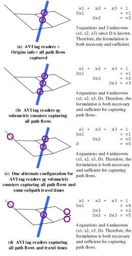
on high-order facilities such as freeways or facilities that require tolls. Data is gathered at (b) AVI tag re aders or
volume tric counters capturing all path fl ows
(c) One al ternate c onfiguration for AVI tag re aders or vol ume tric counters capturing all path fl ows and
some subpath tr avel ti mes (a) AVI tag re aders + Origins info = all path flows
capture d
(d) AVI tag re aders capturing all path fl ows and tr avel times
x1 + x2 + x3 = 1 Dx1 = v1 Dx2 = v2 Dx3 = v3
4 equations and 4 unknowns (x1, x2, x3, D). Therefore, the formulation is both neces sary and sufficient for capturing path flows.
x1 + x2 + x3 = 1 Dx1 = v1 Dx2 = v2
3 equations and 3 unknowns (x1, x2, x3) since D is known. Therefore, the formu lation is both necessary and s ufficient.
x1 + x2 + x3 = 1 Dx1 = v1 Dx2 = v2 D = v0
4 equations and 4 unknowns (x1, x2, x3, D). Therefore, the formulation is both neces sary and sufficient for capturing path flows.
x1 + x2 + x3 = 1 Dx1 = v4 Dx2 = v2 Dx2 + Dx3 = v5
4 equations and 4 unknowns (x1, x2, x3, D). Therefore, the formulation is both neces sary and sufficient for capturing path flows.
7 select locations, missing detailed observations between and beyond collection points. In this example, if a screen line is used connecting the bridge crossings while separating the O and D as in Figure 1.2a, one can measure the path flows and compute the path utilization
coefficients if (n-1) or 2 of the bridges are AVI-equipped with tag readers and one knows the number of vehicles either starting at the O or ending at the D. If no OD information is known, then one would require (n) or 3 tag readers, one for each bridge to observe all
vehicles (Figure 1.2b). However, only spatial paths and not temporal paths will be known in these two cases because there is only one time point for each instrumented path. To measure path travel times on this network, two other cases are shown. Figure 1.2c shows a tag reader network that covers part of the whole network, capturing full path flows and two subpath travel times. To fully collect both spatial paths and temporal paths data, a set-up such as in Figure 1.2d with 4 tag readers would be required. Hence, an AVI system can operate much the same as an AVL system, but with more forethought and hardware required in the planning stages.
8 making assumptions (such as First In, First Out). Therefore, the difference from AVL and AVI is that travel times can never be observed with basic loops because there is no vehicle identification tracking.
Based on this small example, it is evident that path characteristics are difficult to obtain and depend on careful sensor choices and locating. Therefore, a fundamental question that arises is, what data is required to reconstruct a traveler’s path? Once this data is known, then appropriate sensors can be selected to instrument a network. And the problem of where to place the sensors in the network becomes the next step. Focusing on the necessary data, a traveled path has several components, both spatial and temporal:
• Start location • End location
• Start time • End time
• Vehicle trajectory between the start and end locations
• Locations where waiting occurs (say, vehicle is in queue at a traffic light)
• Waiting times
9 Table 1.1 Sensor Attributes Related to Path Reconstruction
TRAFFIC DATA COLLECTION METHOD SENSOR ATTRIBUTES
Legend: symbols are from less to more versatile
zero to full information Lic
e n se P lat e C ou n t S u r ve y F loat in g C ar A e r ial L oop S m ar t L oop A T R V id e o/ L as e r R ad ar G u n T M C A V I (t r an sp on d e r ) A V L ( G P S ) General
Short-term Long-term
Fixed Partially Fixed Mobile
Manual Partially Automatic Automatic
Stand-alone Integrated
Path-specific
Trip Origin
Departure Time
Actual Path / Vehicle Trajectory
Trip Destination
Arrival Time
Potential Proxies
Volume
Individual Vehicle Speed
Direction of travel (heading)
Vehicle Identification
Vehicle Location – facility
Vehicle Location – lane
Note difference between floating car and AVL: floating car here is referring to a controlled field study (often for collecting space mean speed data on particular facilities, not actual trips by the driving population), not in widespread use.
10 are captured. Hence, more fixed detection equipment is required and/or further AVI and AVL detection is necessary. For instance, vehicle trajectory information can be collected:
• Directly from AVL devices.
• Directly from AVI devices and loop detectors fitted with inductive signature recognition equipment (here referred to as “smart loops”) (Ritchie; Abdulhai and Tabib 2003; Sun, Arr et al. 2004) but with a loss of detail between tag readers, and from the origin to the first tag reader and from the last tag reader to the destination.
• Indirectly from laser-based detection systems that yield vehicle lengths and video-based vehicle detection using image processing technology (Oh and Stephen G. Ritchie 2002).
• Indirectly from fixed sensors such as loop detectors that have limited capabilities to collect more than volume, occupancy, and speed information. Basically, these sensors cannot correlate a vehicle crossing one with the same vehicle crossing another one, although there has been some success with using vehicle length measurements on freeway sections (Coifman 1998) and see (Nichols and Cetin 2007). Therefore,
assumptions must be made as to when and where a particular vehicle will cross another fixed sensor.
11 quality, the technique also identifies paths that are missing link count data, suggesting insight into where detectors are required.
1.2 Research Objectives
The research proposed herein is in support of two primary research objectives. First and foremost is the goal of extending the current theoretical frontier of quantifying path flows and their characteristics. This is planned to be accomplished by exploring small networks to start, then creating formulations for increasingly general networks. The second objective is to quantify the tradeoff between direct observation and inference with respect to path flows so that future projects intent on measuring path flows can be guided toward the most beneficial mix of observations and inference based on their available means (for example, current sensors on-hand, available modeling expertise, and budget constraints).
To sum up, here are the objectives in the form of a few guiding questions:
How can transportation engineers and planners more accurately determine the path flows on a network through instrumentation adjustments?
How can the tradeoff between direct observation and inference be quantified? How can route planning be validated?
1.3 Motivation & Research Value
12 accuracy; an agency or firm can only instrument so much of a network. Therefore, it is critical that the tradeoff between efficiency and path flow accuracy be quantified for
personnel to make appropriate decisions. Three examples are briefly presented to highlight the potential impact of path flow knowledge (or lack thereof).
1. What if planners assume inaccurate traffic flows for a region’s future?
Funds may be allocated to “improving” routes that will not be used – a poor decision incurred by ineffective use of resources to develop the flow estimates (wasted dollars).
Insufficient funds may be allocated to routes that will see a marked, unexpected increase in traffic resulting in high v/c ratios and poor levels of service.
2. What if traffic engineers estimate traffic flows with limited accuracy for timing a signal network?
Drivers on roads with higher estimated flows than actual flows have sufficient green time but (1) side streets drivers are forced to wait through unused main street green times and (2) road capacity is inefficiently used.
Drivers on roads with lower estimated flows than actual flows wait in extensive queues at traffic signals with insufficient green times.
3. What if dispatchers route their pick-up and delivery vehicles on tours based on a logistics specialist’s false traffic flow assumptions?
13 If roads on the tour have lower flows than anticipated, then vehicles will arrive early to one or more destinations incurring unproductive time while waiting for the pick-up/delivery time window.
Based on these examples, there is a need for further path flow research. This dissertation is put forth to fulfill that need.
1.4 Paper Organization
Section 2 is a review of select literature addressing four components that shape a picture of path flows and some current methods utilized for determining traveled paths followed by a discussion of the tradeoff between inference and observability when quantifying path flows, and wrapped up with thoughts on gaps in the current literature. Section 3 outlines the
methodology for determining path flows in an instrumented network with descriptions of the applied model, performance measures, and analysis tools. Next, Section 4 includes the experiment design to test the methodology through the random generation of networks then assessed for their instrumentation’s ability to determine the path flows. Section 5 has results of the performance measures for the numerical tests. Finally, concluding remarks and future work are presented in Section 6. Also included are appendices with (a) LINGO
14
2 LITERATURE REVIEW
2.1 Introduction
If all vehicles are instrumented with AVL, then it is a trivial problem to discern the path flows of a network – count up all the vehicles, tally up what paths they were on. However, most transport systems are not and will not be in such a state in the near future. Therefore, discerning path flows in the near term requires using the data available from other
instrumentation configurations. Depending on the type of instrumentation and its network coverage, varying amounts of observability and inference will be required to determine the path flows. One of the goals herein is to quantify the tradeoff between inferring and observing path flows.
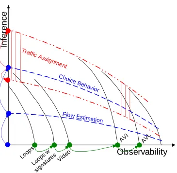
Conceptually, this tradeoff can be plotted as in Figure 2.1. If condition A is present, then there is almost complete coverage of the network with sensors that can yield path flow information (similar to having a high percentage of AVL-equipped vehicles in the network); hence, there is a need for almost no inference to determine the uncovered paths. Being in condition A therefore means that the quality of path flow
discernment should be quite good provided the sensing instruments are reliable. The primary disadvantage of condition A is the high cost of such a
Observability
In
fe
re
n
c
e
C
B
A
15 level of instrumentation, whether it is incurred by transportation agencies and/or by
consumers. Hopefully, the costs will drop over time as technology advances enable more networks to be highly instrumented. In condition B, budget constraints may have hindered a higher level of sensing so more reliance on inference is required. This inference may come in the form of engineering judgment such as applying conservation of flow equations, it may also include information derived from driver surveys, finally, traffic assignment models may be applied to the available data to fill in the gaps. Here in condition B, there is a strong call for quantifying the tradeoff between observability and inference, likely dependent on the type of each one, so that the greatest number of path flows can be distinguished. For instance, a network with 50 percent of links sensed with loop detectors may be better served by inference in the form of an OD survey with route choice questions rather than conservation of flow equations since the survey data asks about what paths a traveler follows through the network; condition B in the survey case is expected to yield a more accurate picture of the path flows than the conservation of flow case. Finally, condition C is the worst possible one with little or no data observed on which to base an estimate of path flows. In this case, the analyst relies heavily on inferring the correct path flows – quite a challenging task with weak substantiation. In summary, quantifying the relationship between observability and inference to create the best estimate of path flows is a key part of this proposed work.
16 track their movements through a network. Further suppose that the path decisions made in the simulation would also be made in the real world (or recognize that this is not the case, but accept the simulated decisions as truth for now). Then the question posed becomes, what output routines must be written so the tagged vehicles’ paths become observable? In other words, the simulation model knows the path truth (for all vehicles), but how can it be extracted? Similar to real-world condition A in Figure 2.1, if one writes a routine that tags 100 percent of the vehicles, then all paths are extracted with little work but at a high expense because processing times are slowed as the number of tagged vehicles increases (likewise in the real world it is costly to tag everyone). Now, if someone uses a routine that tags a percentage less than 100, then some paths are extracted but not all – again, this is similar to condition B because it is less costly but also less data-rich (see Figure 2.2).
100% of trips tagged One outcome of 50% of trips tagged
17
2.2 Examining Relevant Literature
A literature review was conducted to explore how researchers to-date have measured and estimated traffic flows on paths. Discussed below are materials directly related to
quantifying path flows.
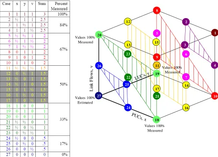
Think of four possible building blocks to create an estimate of network path flows such as in . The lowest and most important building block is that of observed data. Without it, there is no truth. However, as will be discussed later, the available data may not uncover the whole picture of path flows
because of sensor limitations. Therefore, other tools are needed; based on the literature reviewed, three tools are commonly used in transportation engineering: choice behavior, flow estimation, and traffic assignment. As shown in Figure 2.3, these tools can be combined with data in a host of ways to yield path flow estimates. Each building block will be examined in turn and supported by two or more examples from the literature.
2.2.1 Data
As discussed earlier, path flows can be directly obtained through AVL data that captures both spatial and temporal trip information for a particular vehicle – see “Probes as path seekers: a new paradigm” (Demers, List et al. 2006). Data for path flows may also be
D
FE
CB
TA
Legend D = Data
FE = Flow Estimation CB = Choice Behavior TA = Traffic Assignment
Figure 2.3 Path Flow Building Blocks
18 collected via video cameras with overlapping views and the images processed with geometric analysis. Two examples of this empirical method are “Path Detection in Video
Surveillance” (Makris and Ellis 2002) and “Monitoring pedestrians in a [sic] uncontrolled urban environment by matching low-level features” (Vannoorenberghe, Motamed et al. 1996). Both of these papers rely on motion detection research applied to tracking pedestrian movements. Makris and Ellis developed a method based on overlapping and
non-overlapping video images whereas Vannoorenberghe used a single camera with a fixed view in conjunction with a background reference image. From an instrumentation standpoint, these methods require a lot of hardware and generate reams of data for short network segments and therefore are not optimal for large road networks.
However, if instrumentation yielding complete path information (such as AVL devices or video imaging) are unavailable, then data must be obtained from other, less ideal sensors or methods and the paths induced. For example, automatic traffic recorders (ATRs) are
19 better path flow estimates including choice behavior, flow estimation, and traffic assignment – each tool is now discussed in turn.
2.2.2 Choice Behavior
Extending beyond deriving path flows from empirical data has been accomplished by some analysts through translating decisions made by individual travelers into route choice
20 freeway is built), then it is known with high certainty and without field data that this person will likely switch to driving the new freeway instead of arterials connecting relevant OD pairs. Likewise, if a person desires driving the quickest route to a location and it is known how he/she determines that route (such as through radio versus television reports) then researchers can adjust path flow estimates based on the driver’s information being available enroute or only pre-trip. To sum up, choice behavior information can be a powerful asset for quantifying path flows.
Two research teams that incorporated choice behavior for traffic flows are Cascetta et al. (Cascetta, Russo et al. 2002) and Bell and Cassir (Bell and Cassir 2002). The former discusses a route perception model for urban road networks. Recognizing that the choice set varies from individual to individual and few people have a choice set encompassing all possible routes, the authors developed a model incorporating perception that could augment standard route choice models in the traffic assignment process. Therefore, when translating OD flows to path flows it is prudent to consider the impact of traveler perception.
The latter work (Bell and Cassir 2002) viewed route choice through the lens of game theory. While holding onto the assumptions of user equilibrium for the traffic assignment process, uncertainty about route costs is explicitly factored into the choice formulation – implicitly accounting for travelers having a “strategy toward risk”. So in this model, travelers are expected to examine all outcomes prior to selecting a route; in other
CB D
TA D
21 words, they participate in a “mixed-strategy Nash equilibrium of an n-player,
non-cooperative game”.
Related to route choice modeling with some travel demand rules possible, but also some supply side rules, is the category of flow estimation – discussed next.
2.2.3 Flow Estimation
22
D O
Direction of flow
(c) Circuitous paths (b) Se mi-d irect paths (a) Direct paths
T
T T
T
T No trucks
Figure 2.4 Categorizing Paths based on Their Directness
Hence, the difficulty is defining “reasonable” and recognizing that this term will be defined differently when circumstances change. For instance, it is reasonable to assume that
23 Focusing on truck travel further, the authors of a 1994 paper titled “Estimating truck travel patterns in urban areas” (List and Turnquist 1994) applied flow estimation techniques to estimate truck travel patterns. They brought in data from multiple data sources, then determined logical paths by using a geographic information system (GIS) and applying conservation of flow rules. Likewise, again in 2002, List teamed up with Eisenman
(Eisenman and List 2004) to estimate OD matrices with a similar methodology. The
researchers collected data from three sources (probes, link counts, and an old OD matrix) and applied flow logic that included the use of only “reasonable” paths through the network. Based on research such as in the above two articles, insight into the impact of different data sources on the relationship between inference and observability may be possible with the data already collected. In other words, pursuit of such an analysis may quantitatively
indicate how much path observability can be obtained from a data type, enabling the filling in of Figure 2.5 with some concrete results.
Another flavor of flow estimation, that of creating a non-assignment model, is illustrated by a pair of authors who developed an OD model for the specific case of
estimating time-varying OD distributions (i.e. as in the real world, flows between an O and a D change from one time period to the next, such as hourly) (Chang and Tao 1999). Four data types were input into the model including: link and cordon counts, a potentially unreliable prior OD matrix, and path utility coefficients (PUC – the fraction of an OD flow on a unique path).
FE D
24 Finally, an example of flow estimation applied in conjunction with a traffic assignment model is in (Bell, Shield et al. 1997). The flow estimation
component enables links without observed volumes and travel times to have traffic assigned to them based on their capacities and using a penalty (delay) for when a link’s demand is greater than its capacity.
2.2.4 Traffic Assignment
Similar to choice behavior, traffic assignment (TA) is a technique to infer traffic flows when the data available are unable to yield a clear picture on their own. Unlike choice behavior models based on survey data and the logical rules that make up flow estimation, traffic assignment is based on theories of how traffic distributes itself on a network. The primary focus of the technique is on the supply side of traffic with tools including capacity
constraints, link impedance functions, and cases such as system optimal and user optimal equilibrium. Briefly discussed here are some examples from the literature.
Dial’s Probabilistic Choice Algorithm (Dial 1971). Dial created a “multipath assignment model” guided by five functional specifications to try and overcome the shortcomings of the all-or-nothing method (instability, failure to reflect actual behavior) through assigning traffic based on the likelihood of a path being used. Hence, his model was an attempt to assign traffic to a network using common sense assumptions (referred to as flow estimation rules here) and the use of a two-pass Markov model. It is important to note that Dial’s algorithm is not an optimization model like the equilibrium models discussed next.
TA D
FE
TA D
25 On the cutting-edge of TA research today is providing TA in real-time situations, called dynamic traffic assignment (DTA). To do so usually means either sacrificing the theory (relaxing assumptions to simplify and speed calculations) and/ or supplying the system with both expensive equipment (such as high-performance computers with parallel processors) or dividing up the decisions (such as with a bi-level mathematical programming model). Three examples from the literature that utilize DTA are now mentioned.
Chui and Mahmassani creatively updated route guidance via an automaton approach with both data and traffic assignment tools (Chiu and Mahmassani 2003). The researchers applied an a priori math program with updated route guidance given to two classes of drivers.
Focusing on both high performance computing and theory relaxation, another pair of researchers explored the evolution of network flows under route choice dynamics over long time periods such as within-day and day-to-day (Srinivasan and Guo 2004). The DYNASMART dynamic TA model was used to simulate the experiments. User equilibrium was the theory of choice that was then relaxed; it proved to be a wise decision since the results showed the network performed significantly different from equilibrium. Besides TA, this project also included choice behavior with a calibrated route choice model as well as flow estimation elements (such as the link capacity constraints and a modified Greenshields model for speed-density relations).
FE TA D
26 An example of a bi-level programming model that includes a traffic assignment element, specifically stochastic user equilibrium (SUE) is (Xu, Lam et al. 2004). In the lower level, the SUE is part of the “traffic-flow simulator” (TSF) which is Xu and Lam’s equivalent to the path flow estimator (PFE) developed by Bell et al. except the latter team’s initial PFE was based on UE and then modified to incorporate SUE principles (Bell, Shield et al. 1997). So the lower level assigns traffic to the network and updated the OD matrix while the upper level of the program calibrates various parameters of the network to create an integrated model that has feedback between the two problems.
2.3 Summarizing Prior Efforts, Recognizing Gaps in Current
Knowledge
27 Returning to the idea introduced at the beginning of this literature review, the quality and quantity of path flow data is dependent upon a mix of observations and inferences. Often tempered by budget limitations, an analyst needs to maximize the information gained while minimizing the potential for erroneous results by choosing the best combination of
observation instruments and inference tools such as in Figure 2.5. And a mix of
28
Observability
In
fe
re
n
c
e
Loop s
Vide o
AVI AVL
Loop s w
sign atur
es
Flow Estimation Choic
e Beh avior
Traffic Assig
nment
Figure 2.5 The Tradeoff between Inference and Observability
Observability Axis. If the observability axis is comprised of individual sensor types organized from least information gain to most information gain as you move from left to right along the axis and you consider one sensor type at a time, then the quality of your observations improves over this movement. For example, with loop detectors only
29 sensor types, one moves to the other end of the spectrum – Automatic Vehicle Identification (tag readers) and Automatic Vehicle Location (GPS).
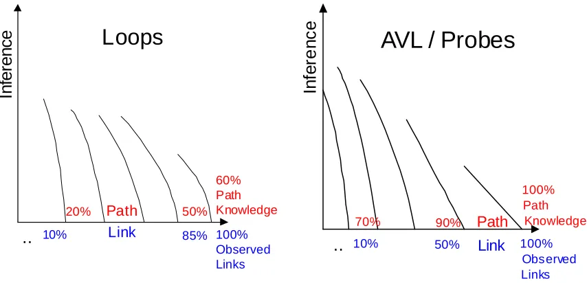
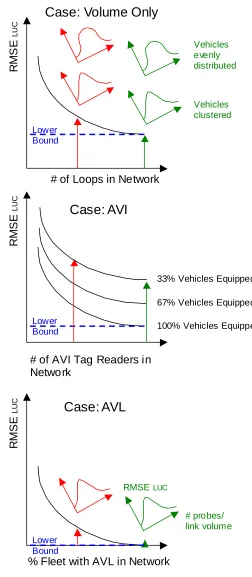
Examining the observability axis further (see Figure 2.6), it is expected that different sensor types will yield varying amounts of path flow information. Consider two base cases (in other words, both without the use of inference), loops versus AVL probes and assume both have zero errors. If 100 percent of a general network is instrumented with loop detectors, then 100 percent of the link volumes will be known; however, 100 percent of the path flows will not be extractable except in very simple networks where FIFO can be proven to hold and where paths do not overlap because again only volumetric data is available with no
30
..
In
fe
re
n
c
e
100% Observed Links
60% Path Knowledge
Link
Path
85%
50%
10%
20%
Loops
..
In
fe
re
n
c
e
100% Observed Links
100% Path
Knowledge
Link
Path
50%
90%
10%
70%
AVL / Probes
Figure 2.6 Potential Inference vs. Observability Graphs for Different Sensor Types
31 estimation since they depend on assumptions that may or may not apply to the network in question. Therefore, these must be handled with utmost care.
Combining Observability and Inference. The third case suggested in the graph is when a combination of each is applied to a given situation, and it is here that a gap in knowledge exists. The type of sensor or combination of sensors will effect the amount of path information available as will the inference tools employed. Although some curves were suggested in this text, they are not backed up by analytical or empirical data; therefore, the actual shape of each curve is suspect. Hence, by examining the tradeoff between
observability and inference for path determination, more clearly defined relationships between different observation instruments and inference tools can be discovered.
2.4 Anticipated Contributions
33
3 METHODOLOGY
34 This dissertation research was guided by the following methodology to address the problem of optimizing the information obtained from sensors given an existing system of detectors on a road network:
1. Develop a mathematical program (MP) to determine path flows.
2. Create or find a road network; preferably with path flow data available for verification.
3. Solve the math program using a set of randomly generated scenarios that involve different levels of stochasticity in the problem inputs.
4. Assess the performance of the math program based on performance measures and comparison to the actual path flows (when available).
5. Repeat this process (steps 1 through 4) – tweaking the math program until it is able to determine the path flows well.
6. Adapt the math program to more complex and realistic network conditions, again by repeating steps (1) through (4) and adjusting the math program to increase its
accuracy and usefulness to the broader community of researchers and practitioners. It is recognized that full path enumeration is only sensible for small networks. Beyond this size, methods such as kth shortest path and column generation that obviate full path enumeration were explored for the implementing algorithm.
35 network for exploratory purposes. That model was refined and its predecessor is specified in Section 3.2 and discussed in detail with the implications of the model specification discussed in subsection 3.2.5, plus several important cases mentioned in subsection 3.2.6. And
potential performance measures to evaluate the math program’s results are described in Section 3.3. Following the methodology is the experiment design (Section 4), then the findings of the analysis conducted so far on 10-node networks (Section 4.1) and concluding remarks (Section 6).
3.1 Problem Functional Specification
Functional specification – the blueprint for the design of a system.1
The proposed functional specifications are as follows:
1. The solution method is to include a mathematical program for optimization. 2. The function of the math program is to determine path flows from an instrumented
network and/or instrumented vehicles using a network.
3. The model should be independent of time, i.e. static in nature to focus on one instant. 4. Conservation of flow shall be upheld throughout the network.
5. The model should be applicable regardless of the network topology. 6. The model should enumerate only the k shortest paths.
1
http://www.techweb.com/encyclopedia/defineterm.jhtml?term=functional+specification Full citation: Technology information about functional specification on both Answers.com and
36 And borrowing three specifications from Dial’s multipath assignment model (Dial 1971):
7. “The model should give all reasonable paths between a given origin and destination a non-zero probability of use, while all unreasonable paths should be given a probability of zero.”
8. “When there are two or more reasonable paths of unequal length, the shorter should have the higher probability of use.”
9. “The model’s user should have some control over the path diversion probabilities.”
It is desired that a model of the following form be developed:
Min z = γAVL(predicted - observed)AVL + γAVI(predicted - observed)AVI + γLOOPS(predicted -
observed)LOOPS
37
3.2 The Model
3.2.1 Notation
- vector of origin-destination flows - flow on arc a
- percent of OD flow on path p (path utilization coefficient) - percent of OD flow on arc a (link utilization coefficient)
od a
p oda
D v x y
- incidence matrix of OD pairs to paths - incidence matrix of odp triplets to arcs , , - weighting factors
= true value of variable m = measured value of variable m ˆ = predict
odp odpa
v x y
m m m
α β
γ γ γ
ɶ
ed value of variable m
3.2.2 Mathematical Program – First Variation (MP1)
Equation 1
Equation 2
Equation 3
Equation 4
3.2.3 General Description
The proposed math program is comprised of one objective function, three constraint
equations, and upper and lower variable bounds as needed. It is formulated as a static model so the complexities of time-dependent OD travel are not yet incorporated at this stage of
ˆ
ˆ ˆ
min
ˆ ˆ
s.t. arcs a
ˆ ˆ
oda triplets ˆ
1 OD pairs
, , , 0
p p
a a oda oda
v y x
a a oda oda p p
odpa p od a
odp
odpa p oda
p
odp p p
a p oda od
x x
v v y y
v y x
x D v
x y
x
v x y D
γ γ γ
β
β
α
−
− + − +
= ∀
= ∀
= ∀
≥
∑
∑
∑
∑
∑
∑
ɶ
ɶ ɶ
ɶ ɶ ɶ
ɶ
38 experimentation. The MP is designed to capture path information from three types of sensor bundles:
1. Fixed-location, volume-only detectors such as loops (point sensors).
2. Fixed-location (at least for a particular model run), vehicle identification detectors such as today’s AVI tag readers.
3. Mobile, vehicle identification, location, speed, and heading detectors such as the current AVL-equipped vehicles (probes).
In Figure 3.1 the MP can be examined in context with the input and output information.
Traffic Inputs
Network Topology Inputs
Weighting Factors
MP Optimization
Traffic Ouputs
Objecti ve Function Ouput
, ,
,
od a p oda
D
ɶ
v
ɶ
x
ɶ
y
ɶ
,
odp odpa
α β
, ,
v x y
γ γ γ
ˆa, ˆp, ˆoda
v x y
Figure 3.1 Flow of Data in the Problem
39 be determined. The objective function is a minimization of three sums ( Equation 1), each of which is the absolute value of the difference between an estimated value minus a choice variable and this difference is then divided by the choice variable to ensure that the magnitude of the difference is captured and not the sign of it. The first sum focuses on the link flows, the second sum is for link utilization coefficients (LUCs), and the third is for the path utilization coefficients (PUCs). Therefore, the quality of the outcome will depend upon which variables are known (measured) and which are estimated through other means. Moreover, any of the three variables (va, yoda, xp) can be the dependent variable. By
minimizing these three variables’ differences the math program is designed to create dependent variables that are closely aligned with their measured counterparts. In other words, an assumption is made that the independent (“~”) and dependent (“^”) variables should not be significantly different, rather one is used to tweak and fill in the gaps of the other. This is a common practice in OD estimation (using a target matrix, see (Sherali, Sivanandan et al. 1994) for one example) but has drawbacks related to the quality of the input OD flows, as will be discussed shortly.
The next three equations constrain the minimization so only reasonable values are allowed. Equation 4 is to ensure that no more and no less than 100 percent (shown in decimal form in the equation) of traffic for a given OD pair is distributed onto the paths used by said pair; in other words, all flows are assigned to a path and the percent of PUCs sum to 100 for each OD pair. The second constraint (Equation 3) ties the path and link utilization coefficients
40 accounted for (and the sum of the PUCs equals the LUC for that link). And Equation 2maps the OD flows to the link flows (conservation of flow equation) by relating the PUCs to the link flows with the understanding that on a given link, and for a given OD pair, the link utilization coefficient will necessarily equal the proportion of traffic between the O and D on all paths that cross the link of interest; hence, the use of the βodpa incidence matrix that maps
each path flow (PUC) to the links traversed.2
Since this model is for a traffic network, both the network’s topology (incidence matrices
αodp and βodpa showing connectivity) and the traffic volumes va must be greater than or equal
to zero so non-negativity constraints are included in the formulation. Moreover, two of the variables, xp and yoda, are proportions having both lower and upper bounds of zero and one,
respectively.
As a whole, some key assumptions are implicit in this formulation. First, fixed sensors can be located along any arc in the network. Second, mobile sensors are associated with the arcs they traverse, but an explicit count of them is not possible (the number of sensors is a higher level issue if this were part of a bi-level problem). Third, monitored arcs have enough sensors for all lanes. Finally, the goal of this MP is to organize all the available sensor data to derive values for path flows (or path utilization coefficients), specifically by seeing how close predicted values can be driven toward observed values. So, this is a data-driven process that assumes matching the observed values is a wise objective. However, it is
2
Paths, like links are numbered consecutively for the entire network. Hence, xp with p = 1 to P and va = 1 to A.
41 recognized that at least two error sources may exist, sensor measurement errors and modeling errors. The former depends on the device used and the conditions of the experiment whereas the latter can depend on coding errors, data entry errors, and incorrect theories. Therefore, this process must be explored to validate whether it is applicable when errors of different types and degrees are present.
3.2.4 Objective Function
As mentioned above, the objective function ( Equation 1) is minimizing the differences of the observed data with the predicted data for link flows, link utilization coefficients, and path utilization coefficients. So the measure of optimality is to minimize the differences between the traffic flow-related input and output variables for the maximum information gain for path flow determinations.
Notice further that the variables are of distinctly different magnitudes with va and Dod being
in terms of vehicle flows (integer) whereas xp and yoda are proportions ranging from 0 to 1,
therefore the magnitudes are normalized through the division of the predicted minus observed differences by the observed values.
Next observe that a variant of the L1-norm is used, but an L2-norm which is computationally easier could also be used. The Euclidean distance or L2-norm,
1
2 2
1 2
1
n p
p
i n
p i
m = m m m
=
≡ ≡ + +
∑
⋯ , is conducive to partials since it is quadratic, but it is42 zero to one range). And, it is important to look at the partial derivatives of the objective function to see how the function will shift with a change in each variable.
Note that the L1-norm,
1
1 1
n p
p i p
i
m = m
=
≡
∑
, will not yield a good partial derivative becausethe absolute value function is not continuous (non-smooth). On the other hand, the L1-norm will allow one to see that there is an ideal shift for each variable (namely,
ˆ , ˆ , and ˆ
v=v yɶ =yɶ x=xɶ). So to enable such discovery, a variation of the L1-norm is included in the objective function.
Finally, weightings of each summation in the objective function are provided for two reasons. Firstly, each variable may or may not be incorporated depending on the available data so the summations of variables can be easily multiplied by a weight of zero to remove them from the objective function without altering the entire model. For example, loop data (va) is easy to acquire so will often be included whereas link utilization data is harder to come
by (it may happen through choice behavior surveys), so the yoda summation may often be
multiplied by zero. Secondly, the weights can incorporate penalties/ costs that could signify error or uncertainty in the observed data.
3.2.5 Implications of the Model
43 origin-destination data is discussed. And third, constraints that could be added are
mentioned.
3.2.5.1 Sensor Type
AVL Sensors. If complete AVL data are available, then all the information needed exists for predicting path flows and the solution is trivial to find; notice that ˆx shows up in every p equation (see MP2 below) so the math program can be driven to a solution with xɶp known. Observe that there are few articles that discuss the AVL sensors with regard to path flows (Schäfer, Thiessenhusen et al. 2002; Nanthawichit, Nakatsuji et al. 2003; Kühne, Schäfer et al. 2003-08; Demers, List et al. 2006); rather, most AVL articles include a treatment of travel time estimation.
ˆ min
ˆ ˆ
s.t. arcs a
ˆ ˆ
oda triplets (MP2) ˆ
1
p p
x
p p
odpa p od a
odp
odpa p oda
p
odp p p
x x
x
x D v
x y
x
γ
β
β
α
−
= ∀
= ∀
=
∑
∑
∑
∑
ɶ ɶ
ɶ
OD pairs ,v xa p,yoda,Dod 0 xp,yoda 1
∀
≥ ≤
44 coefficients or both link utilization coefficients and path utilization coefficients? Another way to look at this is that AVI data provide a second set of point-to-point flows (potentially some OD flows), based on the sub-network covered by the tag readers, plus they provide trip chain information. Therefore, if the researcher’s main focus is on the accuracy of LUCs, there is no added value that the AVI network also provides linked trip information, so the researcher can ignore the path information and only input the sub-network OD flows to provide a lift to the math program thereby improving the quality of the LUCs. However, if the focus is on improving the PUCs, then a second lift can be done by including the linked trip information because these chains are now of immense value. Mathematically, the two variables impacted have additional information from the AVI sub-network that can be shown as follows:
p
od
p od
p subnetwork od subnetwork
x D
D x
x
D − −
⇐ ɶ ⇐ ɶ
ɶ ɶ
ɶ ɶ
In the past seven years, AVI research has picked up with a handful of OD estimation articles now published (Asakura, Hato et al. 2000; Dixon and Rilett 2002; Oh, Ritchie et al. 2002; Antoniou, Ben-Akiva et al. 2004; Dixon and Rilett 2005; Zhou and List 2006).
45 ˆ
min
ˆ ˆ
s.t. arcs a (MP3) ˆ
1 OD pairs
, , , 0
a a
v
p a
odpa p od a
odp
odp p p
a p oda od
v v
v
x D v
x
v x y D
γ
β
α
−
= ∀
= ∀
≥
∑
∑
∑
ɶ ɶ
ɶ
xp,yoda ≤1
46 of arc flows plus the total number of PUCs which equates to (31 + 360 = 391) 391
unknowns. So the problem can be set up with approximately 120 equations and 400 unknowns – clearly underspecified.
As is evident based on the above discussion, it is unlikely with current sensor attribute bundles that only the link utilization coefficients (yoda) will be measured and that the only
term in the objective function would be for the yoda variables. However, LUCs are
commonly included in OD estimation models along with other data (Lam and Huang 1996; Liu and Fricker 1996; Lo, Zhang et al. 1996; Hjorth 1999; Hazelton 2000; Hjorth 2002; List, Konieczny et al. 2002; Lo and Chan 2003).
3.2.5.2 Origin-Destination Data
Addressing the issue of OD-flow data quality is crucial because of the interaction these flows have with link and path flows. Hence, the Dɶod vector3 causes flow shifts in va and
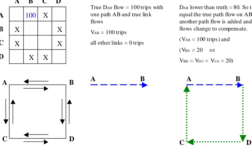
proportional changes to xp and yoda. Looking at the big picture for OD flows, what if the
standard deviation is left alone, but the means for each OD pair are not measured well – now what affects the answer? In other words, the means in the Dɶod vector are shifted uniformly high or low as in Figure 3.2. For example, if given observed link flows and an OD matrix: if an OD matrix flow decreases, then it forces less traffic to generate more volume, therefore more circuitous paths happen so the same traffic covers more links (see Figure 3.3).
3