Scholarship at UWindsor
Scholarship at UWindsor
Electronic Theses and Dissertations Theses, Dissertations, and Major Papers
2016
Practical Guides for Data Retrieval in Deep Web Crawling
Practical Guides for Data Retrieval in Deep Web Crawling
Xu Sun
University of Windsor
Follow this and additional works at: https://scholar.uwindsor.ca/etd
Recommended Citation Recommended Citation
Sun, Xu, "Practical Guides for Data Retrieval in Deep Web Crawling" (2016). Electronic Theses and Dissertations. 5869.
https://scholar.uwindsor.ca/etd/5869
This online database contains the full-text of PhD dissertations and Masters’ theses of University of Windsor students from 1954 forward. These documents are made available for personal study and research purposes only, in accordance with the Canadian Copyright Act and the Creative Commons license—CC BY-NC-ND (Attribution, Non-Commercial, No Derivative Works). Under this license, works must always be attributed to the copyright holder (original author), cannot be used for any commercial purposes, and may not be altered. Any other use would require the permission of the copyright holder. Students may inquire about withdrawing their dissertation and/or thesis from this database. For additional inquiries, please contact the repository administrator via email
Deep Web Crawling
By
Xu Sun
A Thesis
Submitted to the Faculty of Graduate Studies through the School of Computer Science in Partial Fulfillment of the Requirements for
the Degree of Master of Science at the University of Windsor
Windsor, Ontario, Canada
2016
c
by
Xu Sun
APPROVED BY:
Dr. Huapeng Wu
Electrical and Computer Engineering
Dr. Dan Wu
School of Computer Science
Dr. Jessica Chen, Advisor School of Computer Science
I hereby certify that I am the sole author of this thesis and that no part of this
thesis has been published or submitted for publication.
I certify that, to the best of my knowledge, my thesis does not infringe upon
anyones copyright nor violate any proprietary rights and that any ideas, techniques,
quotations, or any other material from the work of other people included in my
thesis, published or otherwise, are fully acknowledged in accordance with the standard
referencing practices. Furthermore, to the extent that I have included copyrighted
material that surpasses the bounds of fair dealing within the meaning of the Canada
Copyright Act, I certify that I have obtained a written permission from the copyright
owner(s) to include such material(s) in my thesis and have included copies of such
copyright clearances to my appendix.
I declare that this is a true copy of my thesis, including any final revisions, as
approved by my thesis committee and the Graduate Studies office, and that this thesis
Deep web crawling refers to the process of collecting documents that have been
organized into a data source and can only be retrieved via a search interface. This is
often achieved by sending different queries to the search interface. Dealing with the
difficulty in selecting suitable set of queries, this crawling process can be implemented
with stepwise refinement: documents are retrieved step by step, while in each step, we
adapt the query selection to our accumulated knowledge obtained from the documents
downloaded in the previous steps. However, it takes much of our time and effort to
download the documents and learn from the resulting sample in order to improve the
query selection. Here we propose a cost-effective, data-driven method for stepping the
adaptive crawling of the deep web. Through empirical study, we explore the criteria
in setting the lengths of the steps to best balance the trade-off between the sample
updating cost and the improved quality of the selected queries. Derived from four
existing data sets typically used for deep web crawling, such criteria provide practical
I would like to express my gratitude to my supervisor Dr. Jessica Chen, for her
valuable assistance and support during my master program.
I also would like to present my appreciation to my committee members, Dr. Dan
Wu and Dr. Huapeng Wu. Thank them for their valuable comments and suggestions
to this thesis.
Meanwhile, I would like to thank Dr. Jianguo Lu and Dr. Yan Wang for collecting
the data sets and providing suggestions on my work.
Finally, I want to thanks to my parents and my friends who give me consistent
DECLARATION OF ORIGINALITY III
ABSTRACT IV
AKNOWLEDGEMENTS V
LIST OF TABLES VIII
LIST OF FIGURES IX
I Introduction 1
II Related Work 5
1 Query Selection Problem . . . 5
1.1 Greedy Algorithm . . . 6
1.2 Weighted Greedy Algorithm . . . 7
1.3 TS-IDS Algorithm . . . 8
1.4 Incremental Queries . . . 9
2 Document Retrieving Strategies . . . 10
2.1 Automatic form filling . . . 10
2.2 Web Database Retrieval . . . 13
2.3 Domain Specific Crawling . . . 14
3 Summary . . . 15
III Background 17 1 Framework of crawling approaches . . . 17
1.1 One-step Sampling Approach . . . 17
1.2 Incremental Approach . . . 18
2 Set-covering Model . . . 19
2.1 Document-term Matrix . . . 19
2.2 Hit Rate and Overlapping Rate . . . 20
2.3 Query Selection Method . . . 21
IV Method 26 1 Overview . . . 26
1.1 Performance Parameters . . . 26
1.2 Revising Cost (k-value) . . . 28
1.3 Stop Criteria . . . 29
1.4 Work Process . . . 30
2 Problem Formalization . . . 34
3 Theoretical Basis . . . 35
3.1 Hypothesis I and Hypothesis II . . . 36
V Experiments 44
1 Experiment Environment and Datasets . . . 44
2 Impact of Parameters . . . 45
2.1 k-value . . . 45
2.2 Unit Sending Cost . . . 46
3 Other Factors . . . 46
3.1 Initial Sample . . . 46
3.2 Create Query Pool . . . 50
3.3 Query Selection Algorithm . . . 50
VI Conclusion 52
REFERENCES 53
1 Example: weighted greedy algorithm . . . 8
2 Example: T S−IDS algorithm . . . 9
1 HTML form in Google deep web crawling . . . 11
2 Text box, selection inputs and presentation inputs . . . 12
3 Work flow of topic focused deep web crawling . . . 15
4 Flow diagram of one-step sampling based approach . . . 18
5 Set covering problem . . . 19
6 Example: Document-term matrix . . . 20
7 Example: query selection . . . 24
8 Flow diagram of work process . . . 31
9 Sample-querynumber relation,α = 0 . . . 33
10 Sample-condition relation, k= 0.001 and k = 104 . . . 34
11 Qual1 and Qual2, sample size = 200, β = 103, k= 10 . . . 37
12 Single step, equal splitting and 10/90 splitting where sample size is 200 and 400 . . . 40
13 Qual1(S1, c), Qual2(S1, c) and Qual3(S1, c) where sample size is 200 and 400 . . . 42
14 k = 10−1, k = 10, k = 103, k = 104 in newsgroup, wiki, reuters and gov2. β is set to 103 . . . . 45
15 β = 102, β = 103, β = 105 in newsgroup, wiki, reuters gov2. k is set to 10 . . . 47
16 Sample-condition relation in differentk−value, β = 103 . . . 48
17 Sample-condition relation in differentβ value, k = 10 . . . 49
18 Weighted greedy algorithm when k = 10−1, k = 10, k = 103, k = 104 in wiki, β is set to 103 . . . . 51
Introduction
Deep web is usually associated with databases or file systems, and the data kept
in the databases or file systems are retrieved using mechanisms different from those
used for surface web. With surface web, data can be accessed directly through URLs.
With deep web, on the other hand, data are guarded by a search interface. Crawling
deep web [6][13][19][26][41] is the process of collecting hidden data by issuing queries
through various interfaces such as HTML forms, web services, programmable web
API, etc. Crawling deep web is helpful when we want to reuse the excavated data, to
provide index to the data, or to build up an integrated environment for search such
data.
Two major issues have been substantially addressed in the literature regarding
deep web crawling. One is about learning and understanding the interface and the
returned result so that query submission and data extraction can be automated
[1][23][33]. Another issue, which is considered in this thesis, is about properly
se-lecting queries to be submitted to the search interface so that the hidden data can be
retrieved cost-effectively and efficiently.
The cost-effectiveness refers to maximizing the coverage of the retrieved
docu-ments in the dataset being considered with minimal cost. Different cost models have
been adopted in previous work [20][30][39][42] reflecting different settings in the real
world. Typically, they include either sending cost or receiving cost, or both, The
sending cost is usually counted using a constant value for each query. It models the
situation where document retrieval is charged by the website service provider on a
each received link. With the assumption that the received links have more or less
the same number of bytes, this provides a simplified model to estimate the total
number of bytes downloaded for the request. It models the situation where the data
transmission over the internet is charged by the service provider of the data plan
on a per-usage basis. In this thesis, both sending and receiving cost are considered.
To keep the model simple, the unit sending cost is defined as the ratio to the unit
receiving cost.
The efficiency is concerned about reducing the time and memory space consumed
for the related computation and document retrieval.
Regarding query selection and data extraction, there are several typical questions:
(a) Where do we get the words to choose from? (b) What criteria do we use to select
the queries? (c) How to find a proper set of queries satisfying the given criteria? A
naive approach is to pick some words randomly from a dictionary. In the past, people
have found it more cost-effective to choose the queries from the terms that frequently
appear in the documents that are stored in the data source being considered. Core
to this proposal is what criteria should be adopted in order to rank the queries for
selection. Much of previous work was dedicated to proposing different solutions to
such criteria with different cost models [30][42].
This query selection scheme naturally leads to the following two-step document
retrieval approach:
• Initially, retrieve a set of sample documents by issuing some words randomly
selected from a dictionary.
• A query pool is built by taking terms appeared in the previous set of sample
documents. Then, a set of queries is selected and issued to the original database.
Clearly, this two-step approach can also be extended into a multi-step one by
re-peatedly refining the sample during the process of document retrieval, i.e. to
repeat-edly select queries, retrieve documents, update sample documents by downloading
newly obtained documents to local database, until certain conditions are met, such
Normally, this adaptive document retrieval process can be more cost-effective
when we take more retrieving steps, because after each sample revision, we are in a
better position to select better queries. However, this requires multiple updates of the
sample, and it usually takes much of our time and efforts to download and analyze
new documents in order to improve the query selection on each step.
Some practical questions arise at this point: What is the optimal number of steps?
If each step may have different length, how to determine the optimal length of each
step?
In this thesis, we introduce the cost of each round of sample revision into the
problem domain, in order to quantitatively measure the trade-off between sending
more queries at a time and sending queries more often. This revision cost is defined
as the ratio to the unit sending/receiving cost, to keep the cost model simple. Note
that: The query here usually refers to the ”phrase” or single keyword in our study.
We use cost limitto define the length of a step. In a simple situation where there is no receiving cost, this cost limit is reduced to the number of queries to select on a step. Based on our cost model, we propose a method to determine, via empirical
study, the optimal lengths of the steps in terms of cost limit. The soundness of this
method is based on three hypotheses. For each hypothesis, we argue why it should
hold, together with some sample supporting data obtained from real datasets.
Through experiments, we have observed that such optimal lengths vary according
to different sizes of the sample dataset. Thus, we repeatedly apply the above method
to obtain the sample-condition relationship i.e. the optimal cost limits according to different sample sizes.
We have applied the above method to four different datasets used for deep web
crawling. The resulting sample-condition graphs demonstrate similar values and their
distribution.
Such obtained sample-condition relationship provides practical guides on the
adap-tive document retrieval: We embed previously obtained sample-condition relationship
into the future crawling of the other datasets. Using such knowledge, the document
the best length for the next step of iteration. With such knowledge, the document
retrieving process will outperform the sample-based and the ordinary incremental
approaches proposed in the literature.
The datasets considered for deep web crawling are normally classified into
text-based documents [10][38][39] and image-text-based ones [2][19][28]. In the present work,
we only consider the data sources that contain plain text documents. Textual data
sources are usually associated with a keyword-based query interface, so the queries
are simply words or phrases, also called terms here. Given that many query interfaces
nowadays offer the advanced search feature to allow users to send multiple-keyword queries, recent work on deep web crawling has seen the consideration of both
single-keyword [4][30][42] and multiple-single-keyword queries [32][41]. For simplicity, only
simple-keyword queries are considered in the present thesis. We leave it open for feature
work to extend the thesis work into the multiple-keyword setting.
The rest of this thesis is organized as follows: In chapter II, we review the previous
research work about deep web crawling. Chapter III introduces the preliminaries of
our method. In chapter IV, we present the new cost-effective document retrieval
method. In chapter V, we show the experiment results using four datasets. We
Related Work
In this chapter, we summarize the related work of our research with more details.
Section 1 reviews several techniques to analyze and select appropriate queries from
sample. In section 2, we introduce some other document retrieving strategies in deep
web crawling.
1
Query Selection Problem
One important problem of deep web crawling is how to generate a set of queries
cost-effectively and efficiently to harvest more documents, i.e determine which queries
should be submitted to a search interface. A simple solution is selecting some random
words from a dictionary. But it fails to consider that a large number of unnecessary
queries with many duplicates would be issued at the same time. Therefore, many
approaches [4][12][30][34][38][39] had been proposed to address the query selection
problem in deep web crawling.
In [4][37], the author study the problem of siphoning hidden data behind simple
search interfaces by issuing keyword-based queries. They suggest that terms presented
in a document collection would generate a set of appropriate queries and these queries
would lead to a high coverage(over 90% is obtained) for most of their sites considered.
Thus, instead of blindly sending queries, they sample HTML forms to select the higher
frequency keywords from a potential keyword list which is expected to lead to a high
coverage in original datasets. In addition, they consider the performance of stop
document collections even though it sometimes turn out to be useless.
Their algorithm consists of two phases: The first phase is to iterate and build
the list of candidate keywords based on their frequency. Once new keywords was
ap-pended into this list, the algorithm modifies the frequency rank of existing keywords.
In phase 2, they select queries with the highest frequency firstly from the term list in
phase 1. They iteratively carry out this process until the coverage in original DB is
no more increased.
1.1
Greedy Algorithm
In [30], the author proposed an efficient sampling-based method to retrieve the most
of entire database in a text data source with low overlapping rate. At the beginning,
they downloaded a set of documents from original DB as the initial sample. From
this sample, a set of appropriate queries was acquired. The query selection process in
sample could be viewed as a set-covering problem which is NP-hard. So they apply
greedy algorithm in experiments to retrieve more documents with a lower cost on
selecting each query. This process is iterated until the selected query set can cover
all documents in sample. It is estimated that those queries which can return most
documents in sample are cost-effective to return most of data in originalDB as well;
The sample size(the number of documents in sample) do not need to be very large in
order to get an accurate enough prediction of the total database. The framework of
this approach is showing below:
1. Create a sample D by initially selecting a fixed number of documents from
originalDB.
2. Analyse the documents and terms in sample D, and build the query poolQP.
3. Select a set of queries Q fromQP based on the greedy algorithm.
4. Issue query set Qto original DB to retrieve documents.
In this paper, the framework aims to select the most cost-effective query. The
number of documents crawled, not the queries issued. So their algorithm focus on
minimizing the overlapping rate. However, in real deep web crawler, sending queries
to original DB may also account for a part of total resources.
1.2
Weighted Greedy Algorithm
In [30], the authors address the query selection problem by cast it as a set-covering
problem. Then they suggest greedy algorithm to generate an optimal query set in
practice. Therefore, each document is of equal importance in their experiments.
However, in real deep web crawling scenario, not every document is the same. That
is because a large document is more likely to be returned than the small documents
which only contain few words.
The initial solution to set covering problem for deep web crawling [30] was
im-proved [38] with the observation that the document-term relationship in this
appli-cation domain follows the power law instead of uniform distribution
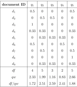
In [38], Wang et al. further improve the straightforward greedy algorithm by
introducing weights into the greedy strategy. Similar to [30], this paper reports
the work on generating an appropriate set of queries so that they can cover all the
documents in sample D with less overlapping rate. In simple greedy algorithm [30],
the unit cost for sending one queryqis set to 1/df, wheredf is the document frequency
of q. The queries are selected one by one. On each step, they select the query with
maximumnew/df, wherenewis the number of new documents that could be retuned
byq. Unlike [30], in weighted greedy algorithm, the authors incorporate weights into
each query selection process, where the weight of a document is the inverse of its
term frequency. The idea behind the weighted greedy method is to select the query
with higher requirement degree as early as possible. The work process of this query
selection strategy is illustrated by the following example.
document ID q1 q2 q3 q4 q5
d1 0.5 0 0 0 0.5
d2 0 0.5 0.5 0 0
d3 1 0 0 0 0
d4 0.33 0.33 0 0 0.33
d5 0 0.33 0.33 0.33 0
d6 0.5 0 0 0.5 0
d7 0 0.5 0 0 0.5
d8 0 0 0 0 1
d9 0 0.33 0.33 0 0.33
df 4 5 3 2 5
qw 2.33 1.99 1.16 0.83 2.66
df /qw 1.72 2.51 2.59 2.41 1.88
TABLE 1: Example: weighted greedy algorithm
1.3
TS-IDS Algorithm
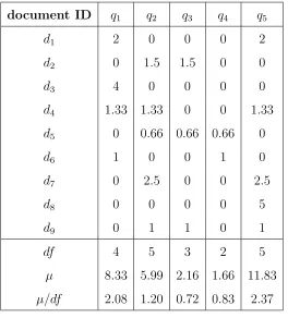
In [39], Wang et al. further modified their weighted greedy algorithm to T S−IDS
algorithm in order to have a better performance in query selection. The authors define
IDS (the inverse of document size) as a measurement of the documents weight, and
T S(term size), as the number of documents it can cover, i.e. the document frequency.
Further, they have assumed that the importance of a document is proportional to the
minimal term size in it. The reason is that: a term with higher T S will bring about
large number of duplicates because more documents could be returned by issuing it
to search interface; On the other hand, small terms are usually with less redundancy
in crawling process. Based on their experiments, the T S −IDS method decreases
the redundancy rate compared with greedy algorithm [30] and IDS algorithm [38]
on a variety of datasets.
Example 2: In the previous example, the unit weight of a document di = df1 ×
query with maximum µ/df will be selected. Here, µ = min(TS). Therefore, in table 2, q5 should be appended to the selected query set.
document ID q1 q2 q3 q4 q5
d1 2 0 0 0 2
d2 0 1.5 1.5 0 0
d3 4 0 0 0 0
d4 1.33 1.33 0 0 1.33
d5 0 0.66 0.66 0.66 0
d6 1 0 0 1 0
d7 0 2.5 0 0 2.5
d8 0 0 0 0 5
d9 0 1 1 0 1
df 4 5 3 2 5
µ 8.33 5.99 2.16 1.66 11.83
µ/df 2.08 1.20 0.72 0.83 2.37
TABLE 2: Example: T S−IDS algorithm
1.4
Incremental Queries
In great majority of incremental deep web crawling approaches, appropriate queries
or HTML forms [17][2] [26][27] are usually selected from documents or web pages
that have been downloaded in previous steps. The number of documents in sample
increases as more queries were sent to original database. This process is iterated until
some terminate conditions were satisfied.
Ntoulas et al. [42] proposed an incremental method on textual database to
gen-erate a near-optimal solution by analyzing and examining the documents returned
from previous steps. The basic idea of this method is that we can approximately get
a good prediction on how many pages or documents will be returned by every word
1. Select a term as initial query q1 and send it to web site.
2. Acquire result index pages and download new documents from internet.
3. Predict the next ‘best’ query, then send it to site for retrieving and downloading
new pages.
4. Iterate this process until some termination criterion is met.
Query selection strategy
In order to generate the optimal query on each iteration, the author estimate the next
potential query qi by:
Ef f iciency(qi) =
Pnew(qi)
Cost(qi)
where P means the fraction of pages that qi can return. Pnew(qi) is the approximate
fraction of new documents that will be returned by qi:
Pnew(qi) = P(q1∨ · · ·qi−1∨qi)−P(q1∨ · · · ∨qi−1)
Cost(qi) represents the total cost of issuingqi to web site, and it can be separated
into three aspects: submitting a query qi, retrieving result pages and downloading
new documents.
Additionally, the authors have reported on their experiments by three policies,
namely random, generic-frequency and adaptive on four real hidden websites. The
results show that their adaptive method is able to retrieve and download most of the
documents in deep websites by sending the least number of queries compared with
the other two policies.
2
Document Retrieving Strategies
2.1
Automatic form filling
In Google’s deep web crawling [32], the authors select good candidates after
developed aims a large coverage in deep web contents, rather than focusing on specific
web sites. Their surfacing method has already been incorporated into Google search
engine, and their results can drive more than a thousand queries per second today.
Form filling
In this paper, a HTML form is defined within a form tag just like figure 2.1. There
<form a c t i o n =‘ h t t p : / / books . com/ f i n d ’ method=‘ g e t ’>
<$ i n p u t t y p e =‘ hidden ’ name=‘ s r c ’ v a l u e =‘hp’>
Keywords : <i n p u t t y p e =‘ t e x t ’ name=‘ keywords ’>
P r o v i n c e : <s e l e c t name=‘ p r o v i n c e ’> <o p t i o n v a l u e =‘Any’/>
<o p t i o n v a l u e =‘ON’/> . . . </ s e l e c t>
S o r t By : <s e l e c t name=‘ s o r t ’> <o p t i o n v a l u e =‘ r e l e v a n t ’/>
<o p t i o n v a l u e =‘ p r i c e ’/> . . . </ s e l e c t>
<i n p u t t y p e =‘ submit ’ name=‘ s ’ v a l u e =‘go ’>
</form>
FIGURE 1: HTML form in Google deep web crawling
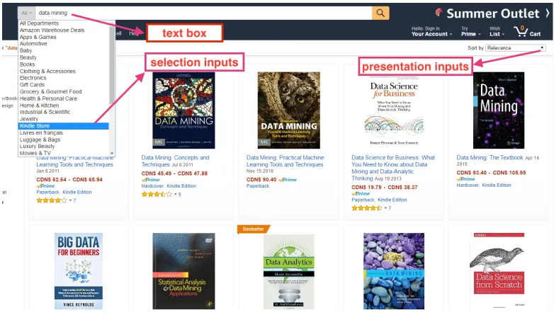
are several input value in the form, but only select menus (selection inputs) and text
boxes (presentation inputs) were considered here. In their work, selection inputs were
usually assigned a wild card value that matches some records in their database. The
presentation inputs is often treated as sort order or HTML layout. Therefore, the
problem of query selection can be seen as the problem of selecting an appropriate
form contents in SQL:
select∗from DB where selection inputsordered by presentation inputs
Also, in their assumptions, the value of text boxes could be a null string, but for
select menus, they assigned a default value as a wild card value. Figure 2 shows what
FIGURE 2: Text box, selection inputs and presentation inputs
Query selection strategy
The purpose of that paper is to receive a good coverage on each web site by issuing
a small number of queries (form submissions). For this reason, they introduce T F
-IDF [35] to select terms from a page after examining the words most relevant to its
contents. In their deep web crawler, T F (term frequency) is a measurement for the
importance of the term on that corresponding web page. IDF (inverse of document
frequency) measures the importance of the word among all possible pages. That is
to say, T F-IDF can balance the word’s significance on the particular page with its
general significance by tf-idf(word, pages) = tf(word, page)×idf(word).
In their experiments, initially, they take top 50 words with the largest tf-idf
value into query pool. Only the top 25 words were added into query pool in next
steps. Furthermore, some useless words with high term frequency (over 80%) or
only appeared on one page will be removed from the query pool. Then they submit
the remaining queries in query pool to original database and a new sample will be
2.2
Web Database Retrieval
As we all know, the majority of web databases are highly dynamic in practical
ap-plications. So a problem has to be addressed about how to maintain the consistency
between the local database and the integrated web database. In [20], the author
proposed an incremental crawling method to update their local database by several
queries generated by their incremental harvest model. That is to say, their work
can be divided into two phases: the first one is how to build the incremental
har-vest model; Second one is selecting the appropriate queries. Furthermore, they define
three measurements to evaluate the performance of their crawler in their experiments,
which areT RC (Total Coverage Rate),ICR (Incremental Coverage Rate) andEF F
(Efficiency).
Incremental harvest model
In their paper, Huang et al. useW DB(ti) to represent all the records in web database
at time ti. So the incremental records between the neighbouring samples, such as ti
and ti+1 can be calculated by:
∆W DB(ti+1) =W DB(ti+1)−W DB(ti)
Next, they build the training sample automatically through these incremental records,
and the incremental harvest model was obtained.
Query selection
The query selection problem is transferred to Set Covering Problem by keeping records
and queries in a document-term matrix. This is similar to [30]. Firstly, the initial
query qi was selected randomly from their initial query list (pool), then some new
records will be retrieved and downloaded to local database by submitting qi to the
web database. Afterwards, an optimal query is iteratively chosen on each step by their
incremental harvest model. This process is terminated when no more new records
2.3
Domain Specific Crawling
From previous work, we know that the only way to crawling deep web data is by
send-ing some appropriate queries to search interface [3][22][36]. Moreover, some strategies
about query selection problem have already been introduced. Most of them usually
focused on receiving the largest coverage in original database, i.e. breadth-first.
Ac-tually, there are also some cost-effective deep web crawling methods for specific topics
[25], i.e. depth-first.
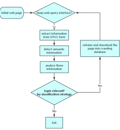
In [9], a Domain specific Hidden Web Crawler (AKSHR) was proposed. Their
framework can be divided into four phases: Firstly, there is a search interface crawling
which can retrieve and store specific search interface by carrying out
domain-specific-assisted approach automatically; The second phase is a domain-specific
inter-face mapping. The authors use the Domain Specific Interinter-face Mapper (DSIM) [8] to
detect the semantic distance between the components of different web interfaces in the
same deep web site. The third phase consists of an automatic form filling which can
generate queries by collecting labels and corresponding values from returned pages;
The last phase is page analysis, which distinguishes whether the result pages returned
by queries on last step is right or wrong. Additionally, they use three measurements
(P recision,Recall, andF −measure) to evaluate the performance of their crawling
results in experiments.
In [21], Jiang et al. provide a deep web crawler framework using machine learning
techniques. Because some existing crawling methods ignored the experience gained
from previous queries, in this paper, they analyze and conclude the environment
information on each given step. Furthermore, the crawler acquires this information
and selects the next query by reward calculation (Q-value) based on the last sample.
Moreover, in [40], the author further proposed a topic specific deep web crawling
method by applying weka as their classification arithmetic to analyze the semantic
webs. They use HarvestRatio as the measurement to evaluate the performance of
their experiment results.
describe by the following figure 3
FIGURE 3: Work flow of topic focused deep web crawling
3
Summary
In this chapter, we have reviewed some research work which are relevant to deep web
incremental approaches [42]. In these two papers, the authors have presented
algo-rithms and results that are very helpful in our work. On the other hand, their studies
may be more reasonable if they take both the sending cost and the downloading cost
into consideration. In our thesis, we would like to add some parameters and criteria
Background
In this chapter, we discuss the preliminaries of our work in two sections. In Section
1, we will show the framework and relationship between one-step sample-based and
incremental approach. In Section 2, we introduce how to transfer the query selection
problem into set-covering problem.
1
Framework of crawling approaches
In this thesis, in order to concentrate on analyzing the performance of one-step
sam-pling approach [30] and incremental approach[42] under different criteria, we build our
own deep web crawler. In addition, we present the framework of these two approaches
in this section to show a rough work process of them.
1.1
One-step Sampling Approach
The framework of one-step sampling approach which is similar to [30], and the work
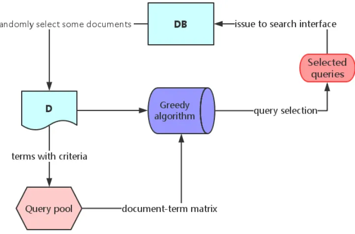
flow diagram is showing in figure 4. Firstly, we randomly collect some documents
as the initial sample D, and query pool QP is created by selecting some terms from
sampleD. Then a query setQwith some appropriate queries are generated and saved
based on our query selection method. After that the corresponding result documents
FIGURE 4: Flow diagram of one-step sampling based approach
1.2
Incremental Approach
With incremental strategies [42], queries are selected step by step, and new documents
are returned and saved as more queries were generated and issued. We follow this
same line of approach here. On first step: We randomly select some documents from
original DB as initial sample D1, which could be the same sample with one-step
sampling approach. Then, a set of optimal queries Q1 will be generated by greedy
algorithm based on the sampleD1. After that, we issueQ1 to original databaseDB,
and a new sampleD2 will be returned and downloaded to our local database. On next
steps: The process similar to the previous step is repeated until some termination
condition is met.
In our studies, the stop criteria could be any cost constraint. Specially, one-step
sampling approach can be seen as one part (first step) of incremental one. However,
the final results of these two approaches should be different in practice. The reason is
resources into pieces in incremental approach. But for one-step sampling approach,
we do not need to do this.
2
Set-covering Model
In our study, the query selection problem is to select a set of appropriate queries
which can cost-effectively retrieve as many new documents as possible with the least
cost. In previous paper [30], it is found out that the query selection problem can be
seen as the set-covering problem (SCP) [5][11][16][29] which is NP-hard [14]. So the
greedy algorithm has been used as a popular solution for this problem.
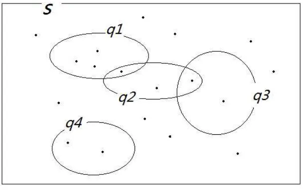
FIGURE 5: Set covering problem
In figure 5, suppose S is the total database with all documents (point) in it. If
a point is in a circle (q), we indicate that this document can be covered or returned
by this query q. Therefore, the query selection problem in dataset S is to find a set
of q (circle) which can cover more documents with a minimal cost. I.e. Set-covering
problem
2.1
Document-term Matrix
Definition 1: (Document-term Matrix)Given a set of documents D =d1, d2,· · · , dm
the document-term matrix A = (aij) where aij = 1 if the document di contains the
term qj, i.e. di can be covered by qj; otherwise aij = 0.
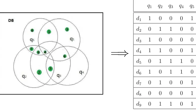
Example 3: A deep web data source DB ={d1, d2,· · · , d9}is shown in figure 6 below,
and query poolQP = {q1,· · · , q5}). Each query is contained in at least one document.
The corresponding document-term matrix is given on the right. One possible solution to this set covering problem is Q = {q1,q3,q5}.
=
⇒
q1 q2 q3 q4 q5
d1 1 0 0 0 1
d2 0 1 1 0 0
d3 1 0 0 0 0
d4 1 1 0 0 1
d5 0 1 1 1 0
d6 1 0 1 1 0
d7 0 1 0 0 1
d8 0 0 0 0 1
d9 0 1 1 0 1
FIGURE 6: Example: Document-term matrix
2.2
Hit Rate and Overlapping Rate
From document-term matrix, we can define hit rate [30] to reflect the cost-effectiveness
of the optimal query set Q in terms of its coverage.
Definition 2: (Hit Rate, HR)Given an m×n document-terms matrix A = (aij)
which comes from a datasets DB = {d1,· · · , dm } and a query pool QP ={ q1,· · · , qn }. A set of queries Q (Q⊆QP) is represented by an n-binary vector X = [X1,· · · , Xn
],Xj = 1 ifqj was selected to Q, otherwise,Xj = 0. Let Y = [y1,· · · , ym] be a binary
m-vector and yi = 1 if Pnj=1aij ×Xj ≥ 1, otherwise , yi = 0. The hit rate of Q in
documents (u) collected by query set Q and the size of datasets DB. u= m X i=1 yi
HR(DB, Q) = u m
Additionally, we define overlapping rate [30] to represent the retrieving cost of all
matched documents by queries in Q.
Definition 3: (Overlapping Rate, OR)Given Q = {q1,· · · , qk}, the overlapping
rate of Q can be calculated by the ratio between the sum of the number of covered documents by each query in Q (v) and the number of of unique documents (u). In terms of document term matrix, this is defined as follows:
OR(DB, Q) = v u
2.3
Query Selection Method
Definition 4: (Query Selection) Given an m×n binary matrix A = (aij), let
Cost(retrieve)= [c1, c2,· · · , cn] be a non-negative n-vector and eachCost(retrievej) = Pm
i=1aij represents the retrieval cost of the query qj. The total cost of query qj is
Cost(qj) = β+Pmi=1aij where β is the ratio of unit cost between sending a query and
receiving a document. Hence, the query selection problem is to search for a binary n-vector X = [X1, X2,· · · , Xn] that satisfies the objective function.
minPn
j=1 Cost(qj)×Xj
Subject to
n X
j=1
aij ×Xj ≥1 (1≤i≤m)
Xj ∈0,1 (1≤j ≤n)
In the document-term matrix of a sample D, each column represents a
Cost(retrievej) is the document frequency of term qj, which is the number of
docu-ments that can be returned by qj.
There are many query selection strategies in deep web crawling, and they can be
divided into three directions [30]:
• Minimize cost
We select the next queryqkwhich has the smallest cost: Cost(qk) = min{Cost(qj)|
1≤j ≤n} and Xj = 0( qj has not been selected yet) on each step. The lowest
total cost for optimal query setQis Pn
j=1(Cost(qj)×Xj), which approximates
the smallest cost.
• Maximum coverage
Another query selection strategy is to select the next termqk to cover the largest
number of rows (documents) which are not yet covered by previous columns
(queries). Namely, if we select qk as the next column (query), setting Xk = 1
to maximize Pm
i=1((1−yi)×aik) where yi ∈ {0,1} and yi = 1 if di has been
returned, otherwise, yi = 0. The largest coverage is approximated by covering
most new rows(documents) on each step.
• New/Cost
In our studies, we combine the previous two strategies together
new cost =
new returned documents by qk
Cost(qk)
One of the issues here is how do we know the number of new documents that
would be returned by qk. Let S(Qk−1) be the set of documents which have
already been returned by previous query set{q1, q2,· · ·qk−1}. We can calculate
S(Qk)−S(Qk−1) by Pmi=1((1−yi)×aik for every potential query in QP, i.e.
the number of new documents that could be retrieved by qk, where yi ∈ {0,1}
and yi = 1 ifdi has been returned, otherwise, yi = 0. Therefore, we have:
new cost(qk) =
Pm
i=1((1−yi)×aik)
β+Pm i=1aik
(1)
Algorithm 1: Query selection algorithm
Input: an m×n matrix A = (aij),β
Output: optimal query set Q
Cost(qj) =β+ m X
i=1
aij
Xj = 0(1≤j ≤n)
yi = 0(1≤i≤n)
while Pm
i=1yi < m do
/* generate the query with maximum new/cost */
for all potential queries qk in QP do
new cost(qk) =
Pm
i=1((1−yi)×aik)
β+Pm i=1aik
end
append qk with maximum newcost(qk) into optimal query set Q
Xk= 1
yi = 1, ai,k = 1 f or (1≤i≤n)
end
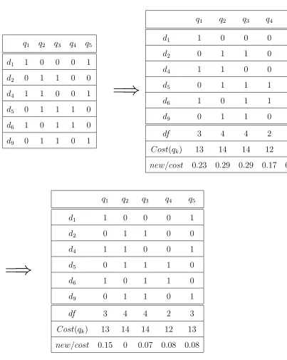
Example 4: Consider the document-term matrix in figure 6 as our original dataset
DB, and β = 10. A random initial sample D is given in figure 7. When we apply algorithm 1 on DB:
q1 q2 q3 q4 q5
d1 1 0 0 0 1
d2 0 1 1 0 0
d4 1 1 0 0 1
d5 0 1 1 1 0
d6 1 0 1 1 0
d9 0 1 1 0 1
=
⇒
q1 q2 q3 q4 q5
d1 1 0 0 0 1
d2 0 1 1 0 0
d4 1 1 0 0 1
d5 0 1 1 1 0
d6 1 0 1 1 0
d9 0 1 1 0 1
df 3 4 4 2 3
Cost(qk) 13 14 14 12 13
new/cost 0.23 0.29 0.29 0.17 0.23
=
⇒
q1 q2 q3 q4 q5
d1 1 0 0 0 1
d2 0 1 1 0 0
d4 1 1 0 0 1
d5 0 1 1 1 0
d6 1 0 1 1 0
d9 0 1 1 0 1
df 3 4 4 2 3
Cost(qk) 13 14 14 12 13
new/cost 0.15 0 0.07 0.08 0.08
FIGURE 7: Example: query selection
1. q2 was selected, which has the largest newcost(q2) = 0.29 in QP, and d2, d4, d5, d9
into Q, P6
i=1yi = 4 < 6. Note: q2 and q3 have the same
new
cost, we randomly
select one of them in this situation.
2. q1 was selected, which has the largest newcost(q2) = 0.15 in QP. After this step, X
= [1,1,0,0,0],P6
i=1yi = 6, so we appendq1 into Q. All documents in sampleD
are covered by Q, so the while loop in algorithm 1 is terminated. Q = {q2, q1}
is returned by our query selection algorithm. The HR(DB,Q) = 89 = 0.89, OR(DB,Q) = 4+5
Method
In the previous chapter, we have shown some preliminary knowledge about deep web
crawling. In this chapter, we present our method. In section 1, we focus on giving an
overview of our method. In section 3, we propose three hypotheses, after which we
explain how to generate a sample-condition relation diagram and the equal splitting
strategy based on these three hypotheses.
1
Overview
In our studies, we aim to provide a guideline for users to choose a more cost-effective
and efficient crawling strategy in crawling deep web. With this objective, we need to
define some parameters to measure the performance of a crawler in different situations,
such as the coverage, cost model and quality. After that, we will explain the work
process of our method in section 1.4.
1.1
Performance Parameters
Coverage in Original Datasets
In our work, the coverage in original dataset DB refers to the ratio between the
number of documents that contain at least one of the selected queries in Q and the
total number of documents in DB, which is defined as hit rate (HR) in [30]. In our
work, we name the coverage inDB asHR(Q, DB), and it can be used to evaluate the
efficiency of a query set Q. Similarly, the coverage in sample D can be represented
calculated as following:
HR(Q, DB) = number of documents containing Q
|DB| (1)
|DB| means the number of documents in original database DB.
Cost Model
As pointed out in many papers on deep web crawler, the crawling cost comes from
many sources, such as the network traffics caused by receiving documents from DB
or the limitation on total number of queries that can be issued by the users daily.
In our work, for each query in Q, the unit receiving cost is represented by α.
Unless explicitly mentioned, in the following, we will use numeric value 1 to denote
the unit receiving cost. The cost of receiving 1000 documents, for example, will be
1000.
The unit cost of sending one query is represented by β, with integer values. When
α is nonzero, it can be viewed as the ratio of the cost between sending one query and
that of receiving one document. If α= 1, β = 1500, and there are 500 documents in
the data set containing term q, for example, the sending cost of q will be 1500, and
the receiving cost of q will be 500. The total cost of q will be 1500 + 500 = 2000.
The cost model for each query is:
Cost(q) =β+α×number of documents containing q (2)
where α is usually fixed as 1 in this thesis.
Quality
LetQbe a set of queries, and D is a data set. The quality of a query q w.r.t. (Q, D)
is measured by the per unit cost return of the number of documents that are obtained
by sending query q to D and that are not obtained by sending any other queries in
Q toD. Note that the cost is calculated for both sending and receiving.
During the query selection process, ideally, we determine the quality of a term
the current sample, and DB is the original data set. However, during the crawling
process, we do not have complete information about the original data set. Thus, we
approximate this quality by measuring the quality of q w.r.t. (Q, S) where Q is the
set of queries already selected by the query selection process during the current round
of iteration, and S is the sample data set. The quality formula of sample S is given
below:
Qual(q, Q, S) = number of new documents
c (3)
A higher value of Qual(q, Q, S) means this q can harvest more new documents with
less resources.
1.2
Revising Cost (k-value)
In the adaptive query selection process, the document retrieval is realized by
itera-tively selecting queries followed by downloading the corresponding documents. This
process is adaptive in the sense that after each iteration of document downloading,
the newly retrieved documents are merged into the sample data set for update before
processing the next round of query selection.
We assume that the queries selected from the updated sample possess better
quality, compared to those selected from the sample without update. There are two
sources that may lead to such quality improvement.
• We have improved knowledge, obtained from the previously downloaded
doc-uments from the same data source, about the terms used in the original data
set. This information is used to enrich the sample for query selection.
• During the query selection process, we determine the quality of a term based on
its quality measured in the sample data set, in order to approximate the same
measurement in the original data set. Such estimation is generally better in the
updated data set.
This adaptive retrieval process requires multiple updates of the sample. Updating
down-loading, and the computational resource consumed to construct the updated matrix,
to generate the query pool, and to select queries.
We use an integer number k to represent the cost of one round of sample update.
When α is nonzero, it can be viewed as the ratio between the cost of one round of
sample update and that of receiving one document. If k = 1000, for example, and
there are in total 5 iterations of sending and receiving in the crawling process, the
total cost for revising the sample data sets will be 1000∗5 = 5000.
Following the stepwise refinement approach, the problem here is how many steps
should we take and how to divide the iteration steps, in order to maximize the overall
result of document retrieval within limited cost budget, or minimize the cost to reach
the quality document retrieval.
1.3
Stop Criteria
In deep web crawling, the queries are usually selected from the query pool sequentially
[30][38][39][42]. There are basically three criteria to terminate the selection:
1. All documents in original datasets are retrieved by Q, or HR(Q, Original) is
high enough, to determinate the crawling process.
2. The crawling process has to terminate due to cost constraint.
3. The set of queries already selected has met the condition for the current round
of iteration
Here we study the best conditions for the third one. Such a condition, called
refine-ment condition, may include, for example:
• the total number of queries already selected
• the hit rate of the set of queries already selected
In our setting, this refinement condition is a cost limit in the sense that: The
query selection process for the current round should terminate if the cost of the
both the cost of sending this query, and the cost of retrieving all the documents that
could be retrieved by this query. The cost of a set of query is the total sum of the
cost of each query in this set.
1.4
Work Process
Through empirical study, we explore the best cost limit for the refinement condition
which determines the length of the steps. Such cost limit varies with different sample
sizes: when the sample is large, the cost limit will be larger, leaving the refinement
condition loose. In this situation, the iteration is in favour of the sample-based
crawling.
Actually, the result of our study is a sample-condition relation (SCR) that
pro-vides the refinement condition based on the sample size. This sample-condition
re-lation provides practical guidelines for cost-effective stepwise refinement in iterative
document retrieval. For example, when sample size is |D|, users can find the
cor-responding optimal cost condition is SCR(|D|) by checking our sample-condition
relation diagram.
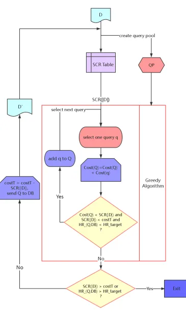
Given a real deep web crawler, with the initial sample D. Using SCR, we can
find that the optimal cost condition is SCR(|D|). Suppose the total cost budget is
costT, HRtarget refers to the target of hit rate in original database. A flow diagram
for users is given in figure 8. Note that when the first query is selected, Q is empty.
The frame work of our method is explained here:
1. Set SCR(|D|) as the cost limit on first round by checking our sample-condition
relation diagram.
2. Apply greedy algorithm onDandQP, then select one optimal queryq, calculate
Cost(q) by formula 1.1.
3. Let Cost(Q) = Cost(Q) +Cost(q), and check whether Cost(Q) < SCR(|D|)
and HR(Q, Original)< HRtarget and SCR(|D|)< costT.
Otherwise, set the total cost budget costT to costT −SCR(|D|). And issue
all queries in Q to DB. New documents will be retrieved and downloaded to
local database to construct new sampleD0. Check the sample-condition relation
diagram, obtain a new cost limit SCR(|D0|) for D0. After that, proceed to the
next round by following step 2 again.
Special Cases
In normal cases, we set αto 1, so β can be treated as the ratio between the unit cost
of sending a query and receiving a document. There are also some special cases we
have to consider.
1. α = 0
In this situation, the cost limit is uniquely determined by the number of queries.
So the refinement condition expresses the constraint on the total number of queries
to select as the length of the step.
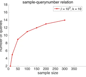
Example 5: Suppose that there is only sending cost and no receiving cost (α = 0). The sample-condition relation is reduced into the sample-querynumber relation.
• Suppose that the sample size is initially 20. According to the sample-querynumber relation in 9, we should select 5 queries for the first round.
• Suppose that the first two stop criteria in section 1.3 are not met, and that after sending the first 5 queries, the sample size is updated into 100. By sample-querynumber relation, we should select 11 queries for the next round.
• Suppose that the first two stop criteria in 1.3 remain unsatisfied. We send these 11 queries in the previous step to DB, and the sample size is updated into 300. According to 9, we should select 14 queries for the next round.
This process is iterated until one of those three terminate conditions in section 1.3.
2. β = 0
In this situation, we do not need to consider the sending cost of each query in Q.
FIGURE 9: Sample-querynumber relation,α = 0
the cost of retrieving URLs as the total cost in their studies. We will to provide more
detail in chapter V to this situation.
3. k →0
When k → 0, the updating cost is almost ignorable. In this situation, the
sug-gested refinement condition is the tightest: terminating the query selection soon. To
the extremist, we could send the queries one by one, updating the sample after each
query.
4. k → ∞
When k → ∞, on the other hand, the update cost is too high that we should
almost always go with the sample-based approach to send out all the queries at once.
The refinement condition in this situation is quite loose so the query selection process
mostly terminates with the first two conditions.
More precisely, a sample-condition relation on newsgroup data set with different
FIGURE 10: Sample-condition relation,k = 0.001 and k = 104
2
Problem Formalization
In our study, based on our cost model, we propose a method to determine the near
optimal lengths of the steps in terms of cost limit. On the other hand, we further
observe that optimal lengths vary according to different sizes of the sample dataset.
Given an initial sample S0 and total cost limit L. The aim of our study is to
determine a positive integer n and positive integers set {x1, x2,· · ·, xn} to maximize
n X
i=1
qi
subject to
n X
i=1
ci < L
where xi represents the number of queries sent on the ith step, i.e. the length of this
step. qi represents the quality obtained by sending xi queries on the ith step. It can
be determined onS0 and{x1, x2,· · · , xi}. ci represents the cost spent on theith step,
onS0 and {x1, x2,· · · , xi}. n is the total number of steps. Given cost limit L,n can
only have finite values. For each value n, variable xi (for 1 ≤ i ≤ n) can only take
finite values. Thus, this is a combinatorial optimization problem.
3
Theoretical Basis
The sample-condition relation is derived from the four data sets used for deep web
crawling. We need to determine, for a given sample size, the best refinement condition
(cost limit).
Let the sample size be fixed. In order to find the best condition, we study the
condition-quality relation with the following two strategies:
• single step strategy
• equal splitting strategy
With the single step strategy, we use the given cost limit c to select queries to
send to the original data set all at once. The quality of these queries is recorded as
the quality of this condition cwith single step strategy.
With the equal splitting strategy, we use 50% of the cost limitcto select the first
part of the queries. This is followed by sample update with costk. Then the second
part of the queries are selected with the remaining cost 50%×c−k. The quality of
the queries from these two parts is then recorded as the quality of this condition c
with the equal splitting strategy.
We use Q(S1, c) to denote the set of queries generated by greedy algorithm from
sample S1 under the cost limit c. With our context, the revising cost for updating
sample is fixed ask. In addition, we define Qual1(|S1|, c) as the quality of single step
strategy by sending Q(S1, c).
Qual1(S1, c) =
the number of new documents covered by Q(S1, c)
c
Similarly, the quality of equal splitting strategy is define as:
Qual2(S1, c) = Qual1(S1,
1
where S2 is the updated sample after issuing Q(S1,12c) to DB.
3.1
Hypothesis I and Hypothesis II
We have the following two hypotheses on the condition-quality relationship. Let c and
c1 be two cost limits. Note that the cost k for updating sample data set is included
in the total cost limit c.
Hypothesis 1: If single step strategy yields better quality than equal splitting strategy w.r.t. (S1, c), i.e. Qual1(S1, c) > Qual2(S1, c), then it would generally also yield
better quality than equal splitting strategy w.r.t. (S1, c1), if c1 < c.
The reason is this: In equal splitting strategy, k is fixed, and the crawler have to
split the cost limitcinto two parts. When cost limit is c1, the available resources for
two parts are 12c1 and 12c1−k respectively, which are both less than 12c and 12c−k
because of c1 < c. Therefore, the revising cost k plays a more important role in c1
than in c. That is to say, compared to c, there are more resource deduction to do
query selection for equal splitting than for single step when cost limit is c1. With less
queries generated, less new documents will be returned. When cost limit is c, Qual1
is smaller than Qual2, so given a smaller cost limit c1, the quality of equal splitting
strategy would generally not be better than single step strategy as well.
Hypothesis 2: If single step strategy cannot yield better quality than equal splitting strategy w.r.t. (S1, c), i.e. Qual1(S1, c) < Qual2(S1, c), then generally it would not
yield better quality than equal splitting strategy either w.r.t. (S1, c1), if c1 > c.
With a larger value of cost limit c1, the revised sample S2 can make a more
accurate prediction to original DB than c, and the cost used in downloading new
sample S2 accounts for a smaller proportion in c1 compared with c. I.e. k has less
impacts on the results of equal splitting strategy. Consequently, for any c1 > c, if
Qual2(S1, c)> Qual1(S1, c), we have Qual2(S1, c1)> Qual1(S1, c1).
Based on these two hypotheses, we compare the condition-quality relations with
step strategy yields better quality than equal splitting strategy: when cost limit is
larger than c, we should split the process into multiple steps.
We look for such refinement condition for a given sample size in this way:
• Use binary search to find a range [a1, a2] such that it contains the refinement
condition and (a2−a1 <∆);
• Use linear interpolation or average to find the refinement condition in range
[a1, a2].
The condition-quality relations with single step and equal splitting strategy on
newsgroup datasets is given below, where sample size is 200.
FIGURE 11: Qual1 and Qual2, sample size = 200, β= 103,k = 10
Example 6: In the above graph, red is from single step strategy and blue is from equal splitting strategy. The maximum cost limit c for single step strategy to be better is around 15000.
Suppose that we start from range [1,28]. The splitting strategy is better for 28, so
the cost limit we are looking for is 2000∗(24−23)/2.
Furthermore, in this condition-quality relation diagram, when c1 < 15000, single
step strategy always yields better quality; when c1 > 15000, equal splitting strategy
always yields better quality. To be more precise, we have listed some corresponding data in Table 3 about this diagram.
cost limit Qual1: single step strategy Qual2: equal splitting strategy
21 169.5650 89.3000
22 130.0387 106.1250
23 88.9537 82.9750
24 49.8272 53.4937
25 26.4997 28.4844
26 14.1763 14.8453
27 7.4150 7.5172
28 3.7420 3.7961
29 1.8745 1.9115
210 0.9385 0.9785
TABLE 3: Qual1 and Qual2, sample size is 200 in Newsgroup
3.2
Hypothesis III
We define the refinement condition c for a given sample size to be the maximum cost
limit for single step strategy to be better than multi-step strategies. Based on the
following hypothesis III, we adopt the condition c obtained from the above method
with equal splitting strategy.
Hypothesis 3: Using other splitting strategy in the above method will yield similar result of cost limit c.
In precious contents, we define Qual1 and Qual2 to measure the quality of single
step and equal splitting strategies. It should be noted that there are many other
1. Also splitting once, but with different percentage for the two parts, e.g. 10/90
splitting, which means the first part of query selection should terminate with
cost limit 10%×c, while the second part terminates with cost limit 90%×c−k.
2. Splitting more than once, e.g. 13/13/13, which means the first part of query
selection should terminate with cost limit 1
3 ×c; the second part terminates
with 13 ×c−k; and the third part terminates with 13 ×c−k.
10/90 Splitting Strategy
For the first situation, compared with equal splitting strategy, although 10/90
split-ting can not generate a good query set on first step, it would have a more accurate
prediction toDB by updated sample on second step. Therefore, if equal splitting have
a better quality than single step with refinement condition c, usually 10/90 strategy
would also outperform the quality of single step strategy as well. On the other hand,
if single step strategy yields better quality than 50/50 strategy, it is usually because
the revising cost k accounts for a large proportion of the cost budget in the crawling
process. Even though 10/90 splitting strategy distribute 90% of its total resources
to the second step, which enriches the second part of the sending and receiving to
yield better result, such benefit is balanced by less improvement of the sample due
to less budget distributed to the first part of sending and receiving. That is to say
the quality of 10/90 splitting would not be much better than equal splitting strategy.
Furthermore, we show an example below.
Example 7: Figure 12 shows condition-quality relationships between single step, equal splitting and 10/90 splitting strategies on newsgroup data set, where β = 103, k= 10. From this diagram, we can find that, no matter in 10/90 or 50/50 splitting strategy, the refinement condition c are within the range of [23,24] and [24,25], respectively for
FIGURE 12: Single step, equal splitting and 10/90 splitting where sample size is 200
Multiple Steps Strategy
Similar to the definition of Qual1 and Qual2, we define Qual3 as the quality for
three-step:
Qual3(S1, c) = Qual1(S1,
1
3c) +Qual1(S
0 2,
1
3c−k) +Qual1(S3, 1 3c−k)
The reason why we apply multiple-step strategy is to select better query and
obtain a more accurate prediction on the original database. When Qual1(S1, c) >
Qual2(S1, c), i.e. the quality of single step is better than two-step, even though we
can receive a more accurate prediction on second step, the growth in quality cannot
cover the cost which was spent in updating the sample. In other words, a large amount
of resources were wasted in modifying the sample. Therefore, when we take
three-step strategy into consideration, the available resources which could be distributed
on each step is less than equal splitting strategy. In addition, the actual cost used in
crawling work is only 13c−k on each step, which was even less than equal splitting
strategy. Hence, normally if Qual1(S1, c) > Qual2(S1, c), Qual1(S1, c) would also be
better than P rod3(S1, c) as well. Analogously, if Qual1(S1, c) < Qual2(S1, c), the
improvement of quality can cover the impact of revising cost on second step. Thus
it usually can cover the impact of revision cost in next steps. Hence, in this case,
the quality of three-step strategy would in general also be better than single step.
Further evidence of these arguments is given in Figure 13.
Example 8: Figure 13 shows the condition-quality relation of one-step, two-step and three-step strategies which is under newsgroup data set, where β= 103, k = 10. Take
all these three strategies into consideration, it suggests that c is in range [23,24] for all the three strategies when S1 = 200, and when sample size is 400, the conclusion
remains the same.
We concentrate on only a part of splitting strategies in our studies. Other strategy
may yield better result sometimes. For example, if 25/25/25/25 is the final split of
total cost budget according to our equal splitting strategy, in some situations, it is
FIGURE 13: Qual1(S1, c),Qual2(S1, c) andQual3(S1, c) where sample size is 200 and
in our experiments. Therefore, we have to point out that some limitations of this
study exists. It is hard for us to try all splitting strategies in our experiments due to
the limitation of computational resources.
4
Summary
In this chapter, we define some parameters to measure the coverage and quality of
different strategies. The purpose of our study is to provide a guideline for deep web
crawler based on our sample-condition relation diagram. Our method is cost-effective
Experiments
In this chapter, we first explain in section 1, the datasets and the environment
set-ting for the experiments. Then we present the sample-condition relation in different
datasets. Moreover, we illustrate the impacts of some parameters on our results in
section 2. Finally, we discuss some issues related to our experiment in section 3.
1
Experiment Environment and Datasets
We write our Java code about query selection based on Lucene [18] package. In
order to show the consistency of our results, we carry out our experiments on four
famous datasets in deep web crawling: newsgroup, Wiki, Gov2 and Reuters. Given
the fixed value of unit sending cost β and revising cost k, we aim to provide a more
cost-effective crawling strategy for users by the way of checking our sample-condition
relation diagram. Our experiment is carried out on a web server with 24 processors.
The original datasets are quite large compared to the computation capability we
have. For example, it takes too much time to build a document-term matrix when we
try to select queries by applying adaptive method. Thus we randomly select 10,000
2
Impact of Parameters
2.1
k-value
In our experiments, we use k to represent the revising cost for updating sample in
adaptive crawling method. The reason is that the adaptive method have to take
a large amount of CPU time and space to retrieve and download new documents
fromDB. After that, we also need to anylyze new sample and do query selection on
it. Therefore, in order to examine how much k affects the sample-condition relation
diagram, we set β to a fixed value 103, and provide the SCR diagram with four
different k values in the following figure 14.
FIGURE 14: k = 10−1, k = 10, k = 103, k = 104 in newsgroup, wiki, reuters and
gov2. β is set to 103
increase of sample size. In addition, when k is increasing, the base of this log function
is increasing as well. That is to say, the cost limit is getting into a fixed value which
increases slowly as sample size increases. This result is in support of our previous
analysis. It demonstrates that when k increases its value, i.e. when it becomes more
and more expensive to perform the sample update, the cost limit will become higher
and higher, which turns more and more in favor of sample-based approach.
2.2
Unit Sending Cost
Recall that β refers to the ratio between unit sending and unit receiving cost in
general. When the unit receiving cost and the unit revising cost are fixed, a higher
value ofβ means the sending cost plays a more important role than revising cost,This
is very similar to the situation whenα and β are fixed andk decreases its value. We
show our SCR diagram with three different β values below.
In the SCR diagrams in figure 15, when β = 102, for example, the relationship
between condition and sample size is similar to the SCR diagram where k = 104 in
figure 14.
A consolidated view on the impacts of k and β on sample-condition relation is
given in figure 16 and figure 17.
3
Other Factors
In our work, we first randomly retrieve some documents from original DB as initial
D. Then theQP is built by choosing some terms from this initial sample. After that,
we select appropriate queries on each step. There are some other factors that affect
our analysis on the step size of the increments in the querying process.
3.1
Initial Sample
About the method to generate initial sample D, we should be aware that we do
FIGURE 15: β = 102, β = 103, β = 105 in newsgroup, wiki, reuters gov2. k is set