The Effect of Multiple Environmental Changes on Crop Model Response and Potential Improvements of Dynamical Land Surface Models

(1)

ABSTRACT

MERA, ROBERTO JAVIER. The Effect of Multiple Environmental Changes on Crop Model Response and Potential Improvements of Dynamical Land Surface Models. (Under the direction of Dev Niyogi and Fredrick Semazzi.)

Agriculture has become a dominant form of land cover through changes in land use,

and is increasingly being considered an important part of land surface and general circulation

models. The objective of this study is to analyze crop models’ responses to multiple changes

in environmental conditions and to provide sources for potential improvements of dynamical

land surface models. We address these goals by evaluating a crop model’s response to

changes in observed climate and future projections from a regional climate model (RCM),

and discerning the effect of multiple environmental changes on C3 and C4 plants.

After successful validation of the model CROPGRO (soybean), we modified

prescribed variations in solar radiation (R), precipitation (P), temperature (T), in the observed

climate for a field experiment’s ambient and enhanced carbon dioxide (CO2) treatments. We

found that the impact of changes in radiation and precipitation is affected by water stress,

while temperature effects differ greatly for varying water-stress conditions and CO2

concentrations.

We then analyzed the model’s responses to data from an RCM simulation for current

and transient increase in atmospheric CO2 levels. Using model data and calculated anomalies,

we found that higher temperatures had a negative impact on crops. We found that higher CO2

reduced the impact of water stress.

Finally, we investigated the effect of individual versus simultaneous changes in R, P,

and T on plant response in a C3 (soybean) and a C4 (maize) plant. Using

(2)

differently for R, P, and T and maize is more sensitive. The results also show that

simultaneous changes in variables do not necessarily agree with individual changes.

Our findings suggest that there is good potential for using the crop models within

dynamical land surface modeling systems for current and doubled CO2 scenarios. Further,

our results indicate that additional considerations for ozone and process-level formulation

(3)

THE EFFECT OF MULTIPLE ENVIRONMENTAL CHANGES ON

CROP MODEL RESPONSE AND POTENTIAL IMPROVEMENTS OF

DYNAMICAL LAND SURFACE MODELS

by

ROBERTO JAVIER MERA

A thesis submitted to the Graduate Faculty of North Carolina State University

In partial fulfillment of the requirements for the Degree of

Master of Science

MARINE, EARTH, AND ATMOSPHERIC SCIENCES

Raleigh, North Carolina, USA

2006

APPROVED BY:

____________________

Dr. Gail G. Wilkerson

Dr. Dev Niyogi

Co-Chair of Advisory Committee

_______________________

Dr. Fredrick H.M. Semazzi

(4)

DEDICATION

To my wife, my parents, and my brothers for their support, encouragement, patience, and

faith in me throughout my studies. For my family and friends, past and present, for helping

me become the person I am today. And to New Orleans, for everything, may it always be my

(5)

BIOGRAPHY

Roberto Javier Mera was born in the city of Guayaquil, Ecuador, in 1978. He moved

to New Orleans, USA, in 1990 where he attended Benjamin Franklin High School and

graduated with honors in 1997. Roberto decided to drastically change the scenery by

becoming a student at the University of North Carolina at Asheville where he would fulfill

his desire to become a meteorologist. After an unfortunate hiatus in 1998 and 1999, he

returned to school in the 2000 fall semester where he continued with his studies in

meteorology. He was in the Dean’s List on several semesters and became a member of the

Sigma Delta Pi National Hispanic Honor Society. During the summer between his Junior and

Senior years, he conducted undergraduate research in Ecuador on the relative economic

effects of the 82-83 and 97-98 El Niño events in that country. He graduated in 2003 with a

major in Meteorology and a minor in Spanish. He began his master’s studies in Atmospheric

Science at North Carolina State University in the fall of 2003. Roberto has served as a

research assistant at NC State and participated in research conducted at Purdue University

and for USDA-ARS. He was accepted as a doctoral student in 2005. His interests include

model skill and value measurements, regional climate modeling, climate-crop model

(6)

ACKNOWLEDGEMENTS

I wish to extend my deepest gratitude to my advisor, Dr. Frederick Semazzi, for his guidance and encouragement through several projects and for supporting and advising me on my academic decisions. I would also like to thank the co-advisor in my committee, Dr. Dev Niyogi for his numerous suggestions for cutting edge research and providing me with opportunities to work with researchers in other scientific areas. I’d like to extend my thanks to Dr. Gail G. Wilkerson of the Crop Science Department at NC State for expanding my knowledge of science beyond the atmospheric realm. I am also grateful for the assistance and input provided by Dr. Noah Diffenbaugh of the Purdue Climate Change Research Center, and Dr. Fitzgerald L. Booker and Walt Pursley of the USDA-ARS Plant Science Research Unit.

I would like to extend my thanks to Greg Buol of the Crop Science Department for the countless hours he spent with me and responding to countless emails to make sure I knew the various configurations, bugs, and benefits of crop modeling. This work would not have been possible without the aid of my colleagues at the Climate Modeling Laboratory; Jared Bowden, Richard Anyah, Baris Onol, Vikram Voojpoojar, and Neil Davis. Without their help I would not have been able to construct the various visuals I used to portray the information in this and other studies, or been introduced to global and regional climate modeling. And finally, I’d like to extend sincerest thanks to my wife, Sara, my family and friends, and to the city of New Orleans for the strength and inspiration that helped me be disciplined and remain committed to my work in the past, present, and future.

(7)

LIST OF TABLES

Chapter 2

Table 1.Definition of variables in multiple interaction simulations………48

Table 2. Average seasonal and monthly weather conditions and CO2 concentrations.

Temperature is in daytime averages and CO2 concentrations are 12 h d_1 (0800–2000 h)

averages……….48

Chapter 3

(11)

LIST OF FIGURES

Chapter 2

Figure1. Observed climate data for the 1999 season. Solar radiation (MJ m-2 day-1) shown in the top plot, precipitation (rain – mm) in the middle, and Max. temp. (°C) (solid line), min. (dashed line) in the bottom plot……….49

Figure 2. Observed climate data for the 2000 season. Solar radiation (MJ m-2 day-1) shown in the top plot, precipitation (rain – mm) in the middle, and Max. temp. (°C) (solid line), min. (dashed line) in the bottom plot……….50

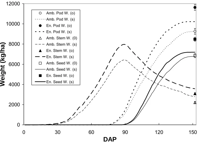
Figure 3. Predicted (lines) versus observed (points) partitioning masses (pod, stem and seed) in 1999. Error bars indicate the confidence intervals in the field experiment………..51

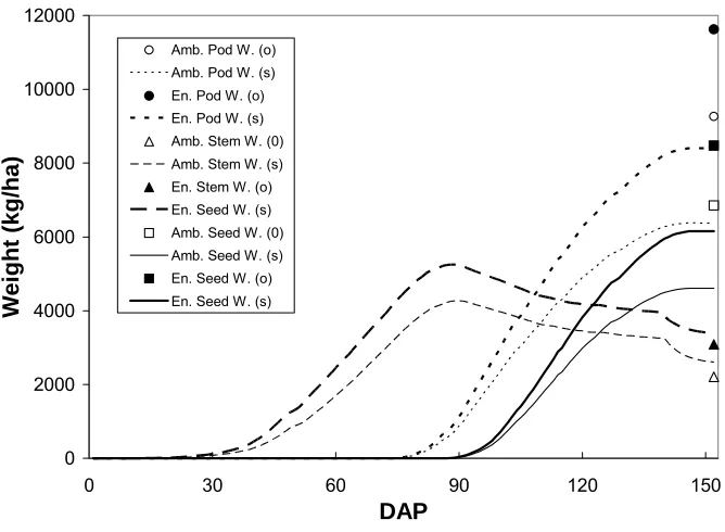
Figure 4. Same as fig. 3 but for 2000………52

Figure 5. Non-linear effects of ambient and enhanced CO2 in irrigated and non-irrigated

environments for 1999 and ambient and enhanced CO2 for 2000. 1999 ambient and enhanced

irrigated simulations have a higher yield at 125% while non-irr. versions are higher between 75 and 100%. The year 2000 simulations seem to prefer radiation levels at 125% for both

ambient and enhanced CO2 conditions………..53

Figure 6. Same as Fig. 5 but for precipitation changes. The relationship is non-linear for the 1999 enhanced CO2 treatments and for both ambient and enhanced treatments in 2000. The plots shows water stress as seen when irrigated treatments in 1999 are compared to the non-irrigated………..54

Figure 7. Same as fig. 5 but for changes in temperature. The effects are non-linear with gradual decreases in yield for non-irrigated 1999 simulations. The 1999 irrigated, enhanced CO2 has a significant peak between 24°C and 26°C, while the ambient gradually peaks at

25°C. The 2000 ambient and enhanced simulations show low yields at 22 that rapidly increase at 23 with small peaks and a gradual decrease thereafter………55

Figure 8 Factor Separation Plot for 1999 Soy Crop Differential Yield (kg/ha). The enhanced (irr) simulation sees the highest impacts by the radiation/precip. (ERP) and radiation/temp

(ERT) interactions, while it is negatively affected by the triple interaction (ERTP). All

simulations follow a similar pattern in positive effects (ERP, ERT) and negative (ET, ERTP ) but

differ in opposite manners when irrigation is changed for EPT and EP. ER is only positive for

irrigated ambient. ………..56

Figure 9. Same as figure 8 but for the 2000 season The enhanced (irr) simulation sees the highest impacts by the radiation/precip. (ERP) and radiation/temp (ERT) interactions, while it

(12)

in positive effects (ERP, ERT) and negative (ER, ERTP ) but differ in opposite manners for EPT,

EP and ET, pointing to an interaction with higher levels of CO2………..57

Chapter 3

Figure 1. Observed climate data for the years 1962-1989. Average annual temperature (°C) on top, and total annual precipitation (mm) on the bottom………..83

Figure 2. Original RCM climate data for the years 2072-2099. Average annual temperature (°C) on top, and total annual precipitation (mm) on the bottom. There is a tendency to a warmer and relatively drier climate as shown by the trendlines………..84

Figure 3. Model anomalies. Average annual temperature (°C) on top, and total annual precipitation (mm) on the bottom. There is a slight trend towards warmer temperatures...85

Figure 4a. Soybean crop yields for observed climate at default CO2 level (solid) and 1989 CO2 level (all in dashed)………..86

Figure 4b. Same as 4a but for transient OBS CO2 levels, c) 2099 CO2 levels, and d) transient A2 CO2 levels (all in dashed)………...86

Figure 4c. Same as 4a but for 2099 CO2 levels………87

Figure 4d. Same as 4a but for transient A2 CO2 levels………87

Figure 5. Annual soybean crop yields for A2 scenario model predictions at default CROPGRO CO2 level and projected 2099 level. ………88

Figure 6a. Soybean crop yields for model anomalies at default CO2 level (solid) and 1989 CO2 level (dashed)………89

Figure 6b. Same as 6a but for transient OBS CO2 levels………..89

Figure 6c. Same as 6a but for 2099 CO2 levels………90

Figure 6d. Same as 6a but for transient A2 CO2 levels……….90

Figure 7. Relationships between soybean crop yields and total yearly precipitation (mm) for observed climate at a) 1989 CO2 level, b) transient OBS CO2 levels, c) 2099 CO2 levels, and d) transient A2 CO2 levels (all in dashed)……….91

(13)

Figure 9a. . Relationships between soybean crop yields (kg/ha) and total yearly precipitation (mm) for future A2 climate at projected 2099 CO2 level (empty circles) and CROPGRO

default level (solid squares). Linear relationships shown for projected CO2 (dotted) and

default (solid)……….93

Figure 9b. . Same as 9a but for average yearly temperatures (°C)………...93

Figure 10. Relationships between soybean crop yields (kg/ha) and total yearly precipitation (mm) for AN model anomalies at a) 1989 CO2 level, b) transient OB CO2 levels, c) 2099 CO2

levels, and d) transient A2 CO2 levels………...94

Figure 11. Same as figure 10 but for average yearly temperature (°C)……….95

Chapter 4

Figure1. Observed climate data (control) for growing season (April 15 through October 15). Solar radiation (MJ m-2day-1) shown in the top panel, precipitation (rain, mm) in the middle, and maximum temperature (°C) (solid line), minimum temperature (dashed line) in the

bottom panel………..132

Figure 2a. Non-linear effects of radiation changes on soybean and maize yield (kg ha-1).

Higher values obtained for the 75% radiation simulation case indicate reductions in global radiation up to a point aids crop yield, and very high or very low values have a negative effect………133

Figure 2b. Non-linear effects of radiation changes on soybean ET (mm) during the different stage of the crop growth. Since ET can be considered a fraction of the incoming radiation, the values are proportional to radiation values………..133

Figure 2c. Non-linear effects of various radiation changes on soybean nitrogen concentration (%). Variation found to be most prominent at day 127, where control value has highest N concentration………134

Figure 2d. Same as Figure 2b, except for maize ET (mm)………..134

Figure 3a. Same as Figure 2a, but for precipitation changes. The relationship is linear, and higher values are shown for 150% precipitation simulation and suggest the importance of higher rain levels to non-irrigated crop yield………..135

Figure 3b. Same as Figure 2b, but for precipitation changes………..135

(14)

Figure 3d. Same as Figure 2d, but for precipitation changes. As with soybean, the higher values are shown by the 150% precipitation simulation……….136

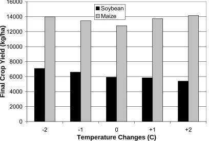
Figure 4a. Same as Figure 2a, but for temperature changes. In these simulations, cooler weather provided higher biomass………137

Figure 4b. Same as Figure 2b, but for temperature changes. For the ranges considered, the corresponding variations in yield were too small for any recognizable trends…………...137

Figure 4c. Same as Figure 2c, but for temperature changes. The impact is more on ET as compared to crop yield………138

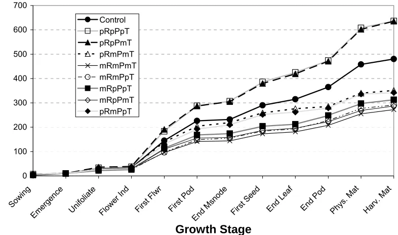
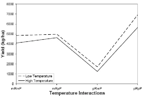
Figure 5. Simulated yields (kg ha-1) for soybean and maize for combinations of different plus

(p) and minus (m) changes in the control values of radiation (R), precipitation (P), and temperature (T)………138

Figure 6a. Similar to Figure 5, but for ET from soybean………139

Figure 6b. Same as Figure 6a, but for a maize………139

Figure 7a. Factor separation Plot for Soybean Crop Differential Yield (kg/ha). A marked trend exists for the radiation-precipitation (EpRpT) interaction to have the largest positive effects. Radiation contribution (EpR) alone gives the lowest differential yield while the triple interaction (EpRpPpT) and temperature (EpT) also appear to have significant negative effects………..140

Figure 7b. Same as Figure 7a, but for maize………141

Figure 8a. Similar to Figure 7a, except for soybean ET………141

Figure 8b. Same as Figure 8a, but for maize differential ET (mm). The same general trend was found as in soybean, with the radiation-precipitation (EpRpP) interaction giving the highest differential ET found in this plot. Radiation (EpR) alone had a much less prominent positive effect while the triple interaction (EpRpPpT) gave the largest negative numbers ………142

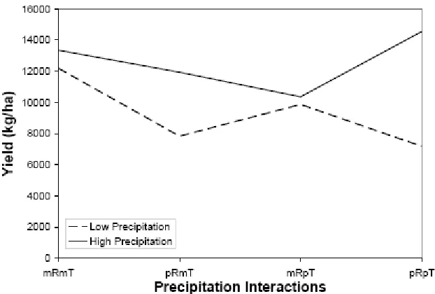
Figure 9a. Summary of interaction between radiation and temperature for high and low precipitation settings results for soybean………...142

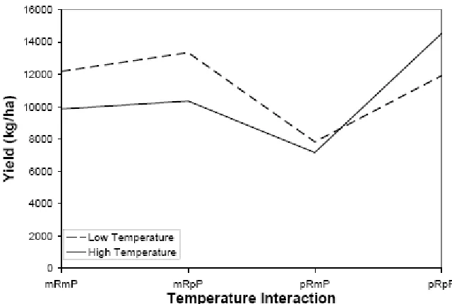
Figure 9b. Same as Figure 9a except for precipitation and temperature interactions under high and low radiation settings for soybean………...143

(15)

Figure 9d. Same as Figure 9a except for maize………..144

Figure 9e. Same as Figure 9b except for maize………..145

Figure 9f. Same as Figure 9c except for maize………...145

Appendices

Figure 1. 1999 Original simulation with altered species file and Norfolk sandy clay loam… ………169

Figure 2. 1999 Simulation using original species file and Appling sandy loam…………169

Figure 3. 1999 Simulation using Appling sandy loam with SLPF coefficient at 1………170

Figure 4. 1999 non-irrigated simulations………171

Figure 5. Same as Figure 1 but for 2000………...171

Figure 6. Same as Figure 2 but for 2000………..………...172

Figure 7. Same as Figure 3 but for 2000………..………...173

Figure 8. Same as fig 4 but for 2000………...173

Figure 9. Radiation changes in altered species and Norfolk soil………174

Figure 10. Same as Figure 9 but for original species and Appling soil (1.27 SLPF)…….174

Figure 11. Precipitation change effects on crops in altered species and Norfolk soil...….175

Figure 12. Same as Figure 11 but for original species and Appling soil (1.27 SLPF)…...175

Figure 13. Temperature change effects on crop yields in altered species and Norfolk soil…. ………176

Figure 14. Same as Figure 13 but for original species and Appling soil (1.27 SLPF)…....176

Figure 15. Factor Separation Plot for 1999 Soy Crop Differential Yield (kg/ha) at altered species and Norfolk soil………..177

Figure 16. Same as Figure 15 but at original species and Appling soil (SPLF 1.27)…….177

(16)

Figure 18. Same as figure 16 but for 2000. ………178

Figure 19. 2000 Season temperature data at -4 degrees of the average seasonal observed temperature (above) and observed (below)……….179

Figure 20. Growth analysis for 2000 season. Seed (grain) weight kg/ha is shown at observed average temperatures and altered (-4C) average temperatures………...180

Figure 21. Daily climate for A2 2097 season in Chapter 3………..181

Figure 22. Same as Figure 21 but for 2099………..182

Figure 23. Growth analysis for grain weight during the 2097 and 2099 seasons for A2

(17)

1. INTRODUCTION

1.1 Agriculture and Land Surface Models

The Earth’s climate is changing due to both natural and anthropogenic forcings (IPCC

2001). Factors such as increasing greenhouse gases, aerosols, and land use changes

contribute to changes in the climate. Droughts, floods, and weather extremes such as severe

storms or prolonged periods of unseasonably cold or warm temperatures can have a

significant effect on agriculture. Agriculture is one of the most climate-sensitive fields, but

recently it has been found that its reciprocal effects on the environment could be a potential

contributor to climate change (Rosenzweig and Parry, 1994; Foley et al., 2005). Possible

changes in the climate due to land cover/land use change (LCLUC) and increases in carbon

dioxide (CO2) could provide increased complexity in patterns of regional productivity, and

the changes that its feedbacks may incur in the atmosphere.

The potential benefits of analyzing a crop’s response to changes in the climate could

help diagnose how modifications in agricultural patterns may affect the atmosphere.

Agriculture plays a major role in regional climate change through its influence on LCLUC.

These changes, in turn, affect agricultural productivity through changes in the environment.

Global climate model (GCM) results have been shown to have inadequate spatial scales to

adequately address these potential changes because of their coarse resolution (Gates, 1985;

Robinson and Finkelstein, 1989; Lamb, 1987; Smith and Tirpak, 1989; Cohen, 1990). There

is a considerable mismatch of scales between coarse resolution GCMs (100s of km) and the

scales of interest for regional impacts (at least an order magnitude finer scale) (IPCC, 1994;

Hostetler, 1994). For instance, mechanistic models (e.g. CROPGRO, CERES-Maize)

(18)

resolutions varying from single plants to a few hectares (Mearns et al., 2003). Results from

these models may be highly susceptible to fine-scale climate variations that may be

embedded in coarse-scale climate variations, especially in regions with complex topography,

coastlines, and in those with highly heterogeneous land surface covers (Mearns et al., 2003).

The addition of agricultural effects on the environment has been explored to diagnose

its impact on climate at the regional scale (Tsvetsinskaya et al., 2001; Feddema et al., 2005).

Statistically significant changes (at the 0.05 level) in latent heat and sensible heat have been

found in extremely dry conditions as a response to changes in leaf area index (LAI) values

through the incorporation of crop model processes from CERES-maize (Tsvetsinskaya et al.,

2001). Other important variables, such as evaporation and transpiration, were also found to

be affected by changes in LAI. This effect followed a distinct diurnal pattern that was more

pronounced in drier conditions.

The study by Feddema et al. (2005) shows that agricultural expansion under the

International Panel on Climate Change (IPCC) Emissions Scenario A2 scenario had

significant effects in the mid-latitudesproducing cooler temperatures with a smaller mean

daily temperaturerange over many areas. It was also found that the A2 scenario, with

elevated values of CO2, produced significant changes that were often opposite those in the B1

(lower CO2 levels) scenario.

Unlike previous research that compared past and present climates through the

inclusion of potential and current vegetation, respectively, a recent study focused on the

evolution of vegetation distribution in the United States for the past 300 years (Roy et al.,

2003). The study utilized NASA’s Ecosystem Demography (ED) computer model, which

(19)

the expansion of agriculture since 1700 caused significant cooling (~0.5C) in parts of the

Great Plains and Midwest. It is believed that temperature changes in the mid-latitudes has

occurred due to increases in evapotranspiration from farmlands as well as increased surface

albedo (Sellers et al., 1996; Betts, 1999; Bonan, 1999; Zhao et al., 2001; Roy et al., 2003; de

Noblet-Ducoudré, 2005).

Past studies also show that a projected lengthening of the growing season in

mid-latitudes (Myneni et al., 1997) could result in increases in biomass density, biogeochemical

cycling rates, photosynthesis, respiration, and fire frequency, thus leading to considerable

changes in albedo, evapotranspiration, hydrology and carbon balance (Bonan et al., 1992;

Thomas and Rowntree, 1992; Harding and Pomeroy, 1996; Levis et al., 1999). A number of

studies have also focused on interactions between climate and vegetation over the tropics,

where conversion of forests to grasslands and croplands has been occurring for years (e.g.,

Nobre et al. 1991; Xue and Shukla 1993; Polcher et al. 1996).

The role of farmlands in the global scale has also not been considered in studies such

as Dufresne et al. (2002), Friedlingstein et al. (2003), and Cox et al. (2000), where the

interactions between land surfaces and increasing levels of CO2 was explored. Global

biosphere models summarize natural biogeochemical and biophysical processes to simulate

important ecosystems processes (e.g., photosynthesis, respiration, etc.) at a large spatial

scale, and are often designed to be coupled with atmospheric general circulation models

(GCMs) (Gervois et al., 2004). These global models generally have few plant functional

types, and they treat croplands in a simplistic manner.

Indeed, recent studies have suggested that croplands effects on the atmosphere may

(20)

intensity of tornadoes through high levels of transpiration (D. Niyogi, Personal

Communication, 2006). As is the case with global models, the majority of research seeking

to address the impact of land use on regional scales has treated croplands as “modified

grasslands.” Crop models, which are able to represent agroecosystems realistically, have only

been tailored for specific predictions and analyses at the site or field level, and their

incorporation into global and regional models has seldom been considered (Gervois et al.,

2004).

There is a need for closer coupling between models of climate, crops and hydrology,

in order to get better representations of climate change. Recent research has aimed at

acquiring crop-specific information for dynamical land surface models through the use of

crop models (Gervois et al., 2004; Betts, 2005). There have been studies performed

integrating crop models into land surface models for global scales (Gervois et al., 2004;

Osborne, 2004), and regional scales (Pan et al., 2004a; Pan et al., 2004b). This type of

research has shown promising results that suggest additional work is necessary for

introducing crop models to land surface models in order to attain proper representation of

cropland-climate interactions. Areas with heterogeneous landscapes are critical to

reproducing important features of the climate, and applications within these regions require

RCMs with the capability to discern fine-scale processes (Mearns et al., 2003). Regions with

heterogeneous land surfaces include the southeastern US, the Sahael, and inland Australia,

where high resolution modeling is highly recommended (given a particular context, resource,

and study goal) (Mearns et al., 2003).

Our aim in this study is to analyze a crop model’s response to multiple changes in the

(21)

and thus acquire a representation of key aspects that should be taken into consideration for

the integration of crop modeling systems within dynamical land surface modeling systems.

We present this approach through the description of our study (section 1.2).

1.2 Description of Study

Greenhouse gases have increased exponentially since the industrial revolution (IPCC,

2001). Climate simulations using GCMs have consistently predicted large scale climatic

responses due to increases in greenhouse gases like CO2 from anthropogenic sources (IPCC,

2001; Meehl et al., 2005). The impact of increasing CO2 on agriculture has been major focus

of climate change studies. A wide variety of field experiments have shown that increased

CO2 tends to stimulate plant growth (Cure and Acock, 1986; Bazzaz, 1990; Rogers and

Dahlman, 1993; Rogers et al., 1994; Drake et al., 1997; Curtis and Wang, 1998; Ainsworth et

al., 2002; Jablonski et al., 2002; Booker et al., 2005). Another group of studies has shown

that plant responses may vary by considerable amounts, due mainly to differences in

experimental protocols and genotypes, and plant growth environment (Ainsworth et al.,

2002; Fiscus et al., 2001; Kimball, 1983; Eastman et al., 2001; Niyogi and Xue, 2005).

Crop models provide a method to test multiple changes in environmental conditions

to construct future projections of agricultural productivity. For instance, the model

CROPGRO (soybean), has been used to discern the effect of elevated levels of CO2 has on

soybean crops (Cavazzoni et al., 1997; Boote et al., 2002a; Wolf, 2002a; Alagarswamy et al.,

2006). These studies, however, have not addressed how simultaneous changes in weather

variables such as precipitation (P), solar radiation (R), and temperature (T) may interact with

(22)

compare the crop model’s response to individual and simultaneous changes in climate

parameters in enhanced and ambient CO2 conditions, irrigated and non-irrigated treatments,

and mixtures of the two. For this, we use observed weather data from a field experiment after

successful model validation.

Regional climate models (RCMs) present an alternate way to test CROPGRO’s

response to environmental changes. They have been shown to be superior to GCMs through

their ability to enhance spatial and temporal differences in crop performance trough higher

resolution (Semenov and Jamieson, 2000; Cocke and LaRow, 2000; Guerreña et al., 2001).

Recent studies suggest that RCMs have the ability to approximate regional and localclimate

change scenarios that would enable application for predicting impacts on agriculture (Giorgi

et al., 2001; Hanley et al., 2002). RCMs have previously been used to drive crop models for

climate change sensitivities and elevated CO2 effects (Guerreña et al., 2001; Hanley et al.,

2002; Adams et al., 2003; Carbone et al., 2003; Tsvetsinskaya et al., 2003).

Recent advances in regional climate modeling have allowed for higher resolution

scales that can capture fine scale processes that may influence regional and local responses to

changes in large scale patterns due to anthropogenic and non-anthropogenic causes

(Diffenbaugh et al., 2005). Such fine scales could prove beneficial for coupling the RCM

with a crop model by creating more representative local conditions, and reproducing climate

extremes that may be useful in analyzing a crop’s response. In our second study, we will use

RCM data to drive CROPGRO at a variety of CO2 concentrations to discern the impact of

climate change on the relationship between crop yields and environmental variables like soil

moisture, precipitation, effective precipitation, and temperature. We develop model

(23)

compare them against model runs using observed weather data and original RCM

projections.

Recent studies suggest that different aspects of climate change (e.g. solar radiation,

precipitation, and temperature) should be addressed beyond increasing amounts of CO2 on

regional productivity (Hansen et al., 2002; Pielke et al., 2001). Variations in atmospheric

radiation can alter hydrological cycles (Ramanathan et al. 2001), the carbon cycle (Niyogi et

al. 2004), and evapotranspiration (Pielke et al. 2001). Earlier studies suggest that

precipitation is the leading climatic factor affecting crops (Rosenzweig and Tubiello, 1997;

Iglesias et al., 1996). It’s been shown that water deficit can reduce the overall biomass of

soybean, regardless of CO2 enrichment (Ferris et al., 1999). Studies of crop’s responses to

climatic factors have made it evident that complex interactions due to precipitation patterns

greatly impact regional productivity.

In addition to the study of precipitation changes, a number of studies have also

focused on the influence that radiative changes may have on crops. Such work has focused

on crop sensitivity to ultraviolet radiation (Bookeret al., 1992; Fiscus et al., 1994; Miller et

al. 1994; Mark and Tevini, 1997), and radiative properties like diffuse radiation (Chamedies

et al. 1999; Niyogi et al. 2004). Biospheric productivity and structure could be impacted by

increasing aerosols and clouds due to biomass burning or volcanic eruptions (Hansen et al.

1999; Gu et al. 2003). The natural and anthropogenic aerosols could contribute to reduction

in the solar radiation absorbed by the Earth’s surface by absorbing solar radiation, and

reflecting it into space. A study by Pielke et al. (2005) suggests that this could produce a

redistribution effect on surface heating and could change agricultural productivity in certain

(24)

Temperature is another factor that can affect agricultural productivity (Fiscus et al.,

1997). Changes in temperatures influences photosynthesis, respiration, transpiration rates,

plant development, and sugar storage. Complex interactions betweenchanges in radiation

and temperatures can incur a variety of effects. Increasing aerosols can typically reduce

surface temperatures by lowering surface radiation levels. The composition of the aerosols

adds to the complexity of this interaction, since carbon dominated aerosols may cause

warming while sulfate aerosols may induce further cooling (Pielke et al., 2005).

Water vapor pressure deficits in the air can be affected by changes in temperature,

thus impacting the water use from agricultural landscapes (Kirschbaum, 2004). This

feedback can cause considerable modifications in temperature and evaporation/transpiration

through changes in transpiration and contribute to regional changes in precipitation and

cloudiness, leading to changes in radiation (Pielke et al., 2001). Thus, it is important to

recognize that environmental changes other than increasing CO2 levels (e.g. radiation,

precipitation, temperature) should be considered for their effect on regional productivity.

Past studies have shown the potential for interactive effects of multiple environmental

factors on the plants’ response by assessing the role of multiple effects and isolating

individual impacts of climate change (Kirschbaum, 1994; Idso & Idso, 1994; Ham et al.,

1995; Drake et al., 1997; Eastman et al., 2001). Thus, in the third part of the study, we seek

to develop an analysis to evaluate the individual and multiple interactions of radiation,

temperature, and precipitation changes on regional productivity of C3 (soybean) and C4

(maize) crops.

We present our study as follows. Section 2 discusses crop model sensitivity to

(25)

the effect of environmental forcing on improving dynamical land surface models by testing a

crop model with data from an RCM. In section 4 we explore potential individual versus

simultaneous climate change effects on soybean (C3) and maize (C4) crops through the use of

an agrotechnology Model. Conclusions are presented in section 5, and an appendices are

(26)

REFERENCES

Adams, R. M., McCarl, B. A., Mearns L. O. 2003. The effects of spatial scale of climate scenarios on economic assessments: An example from U. S. agriculture. Clim. Change.60, 131-148.

Alagarswamy, G., Boote, K.J., Allen, L.H. Jr,. Jones, J.W. 2006. Evaluating the CROPGRO– Soybean Model Ability to Simulate Photosynthesis Response to Carbon Dioxide Levels. Agron. J. 98, 34-42.

Ainsworth, E.A., Davey, P.A., Bernacchi, C.J., Dermody, O.C., Heaton, E.A., Moore, D.J., Morgan, P.B., Naidu, S.L., Ra, H.-S.Y., Zhu, X.-G., Curtis, P.S., Long, S.P. 2002. A meta-analysis of elevated [CO2] effects on soybean (Glycine max) physiology, growth

and yield. Global Change Biol. 8, 695–709.

Bazzaz, F.A. 1990. The response of natural ecosystems to the rising global CO2 levels. Annu.

Rev. Ecol. Syst. 21, 167–196.

Betts, R.A., 1999. The impact of land-use on the climate of present day. Research activities in atmospheric and oceanic modeling, CAS/JSCE WGNE Rep. 28, WMO, Geneva, Switzerland, 7.11–7.12.

Betts, R.A., 2005. Integrated approaches to climate–crop modelling: needs and challenges. Philosophical Transactions: Biological Sciences. 360, 2049 – 2065.

Bonan, G.B., Pollard, D., Thompson, S.L. 1992. Effects of boreal forest vegetation on global climate. Nature.359, 716–18.

Bonan, G.B., 1999. Frost followed the plow: Impacts of deforestation on the climate of the United States. Ecol. Appl. 9, 1305-1315.

Booker, F.L., Miller, J.E., Fiscus, E.L., 1992. Effects of ozone and UV-B radiation on pigments, biomass and peroxidase activity in soybean. In: Berglund, R.L. (Ed.). Tropospheric Ozone and the Environment: II. Effects, Modelling and Control Air and Waste Management Association, Pittsburgh, PA. pp. 489-503.

Boote, K. J, Batchelor, W.D, Jones, J. W. 2002a Project planning and work session. Griffin AES, Griffin, GA.

Carbone, G., Kiechle, W., Locke, L.,Mearns, L., McDaniel, L., Downton, M., 2003, Response of soybeans and sorghum to climate change scenarios in the southeastern United States. Climatic Change, 60, 73-98.

(27)

Chameides, W.L., Yu, H., Liu, S.C., Bergin M., Zhou, X., Mearns, L., Wang, G., Kiang, C.S., Saylor, R.D., Luo, C., Huang, Y., Steiner, A., Giorgi,F., 1999. Case study of the effects of atmospheric aerosols and regional haze on agriculture: An opportunity to enhance crop yields in China through emission controls? PNAS.96, 13626-13633.

Cocke, S., and T. E. LaRow, 2000. Seasonal predictions using a regional spectral model embedded within a coupled ocean–atmosphere model. Mon. Wea. Rev. 128, 689– 708.

Cohen, S.J. 1990. Bringing the global warming issue closer to home: the challenge of regional impact studies. Bull. Am. Met. Soc.71, 520-526.

Cox, P. M., R. A. Betts, C. D. Jones, S. A. Spall, and I. J. Totterdell, 2000. Acceleration of global warming due to carbon-cycle feedbacks in a coupled climate model. Nature.

408, 184–197.

Cure, J.D., Acock, B. 1986. Crop responses to carbon dioxide doubling: A literature survey. Agric. For. Meteorol. 38:127–145.

Curtis, P.S., Wang, X., 1998. A meta-analysis of elevated CO2 effects on woody plant mass,

form, and physiology. Oecologia. 113, 299-313.

de Noblet-Ducoudré, N., Gervois, S., Ciais, P., Viovy, N., Brisson, N., Seguin, B., Perrier, A. 2005. Coupling the Soil–Vegetation Atmosphere Transfer Scheme ORCHIDEE to the agronomy model STICS to study the influence of croplands on the European carbon and water budgets. Agronomie., in press.

Diffenbaugh, N.S., Pal, J.S., Trapp, R.J., Giorgi, F. 2005. Fine-scale processes regulate the response of extreme events to global climate change. PNAS, 102, 4415774–15778.

Drake, B.G., González-Meler, M.A., Long, S.P.. 1997. More efficient plants: A consequence of rising atmospheric CO2? Annu.Rev. Plant Physiol. Plant Mol. Biol. 48, 609–639.

Dufresne, J.-L., Fairhead, L., LeTreut, H., Berthelot, L., Bopp, L., Ciais, P., Friedlingstein, P., Monfray, P. 2002. On the magnitude of positive feedback between future climate change and the carbon cycle. Geophys. Res. Lett. 29, 1405,

doi:10.1029/2001GL013777

(28)

Feddema, J.J., Oleson, K.W., Bonan, G.B., Mearns, L.O., Buja, L.E., Meehl, G.A., Washington, W.M. 2005. The Importance of Land-Cover Change in Simulating Future Climates. Science. 310, 1674 – 1678.

Ferris, R., Wheeler, T.R., Ellis, R.H., Hadley, P., 1999. Seed yield after environmental stress in soybean grown under elevated CO2. Crop Sci. 39, 710-718.

Fiscus, E.L., Miller, J.E., Booker, F.L., 1994. Is UV-B a hazard to soybean photosynthesis and yield?: Results of an ozone/UV-B interaction study and model predictions. In: R.H. Biggs and M.E.B. Joyner (Eds.) Stratospheric Ozone Depletion/UV-B Radiation in the Biosphere Springer-Verlag, Berlin. pp. 135-147.

Fiscus, E.L., Reid, C.D., Miller, J.E., Heagle, A.S., 1997. Elevated CO2 reduces O3 flux and O3-induced yield losses in soybeans: possible implications for elevated CO2 studies. J. of Exp. Botany. 48, 307-313.

Friedlingstein, P., Dufresne, J.-L., Cox, P.M., Rayner, P. 2003. How positive is the feedback between climate change and the carbon cycle? Tellus. 55B, 692–700.

Gates, W.L., 1985. The use of general circulation models In the analysis of the ecosystem impacts of climatic change. Clim. Change. 7, 267-284.

Gervois, S., de Noblet-Ducoudré, Viovy, N., Ciais, P., Brisson, N., Seguin, B., Perrier, A. 2004. Including Croplands in a Global Biosphere Model: Methodology and Evaluation at Specific Sites. Earth Interactions. 8, 1-25.

Giorgi, F. et al. 2001. Regional Climate Information: Evaluations and Projections. Chapter 10 in Houghton et al., IPCC Third Assessment Report. The Science of Climate Change, Cambridge University Press, pp 583-638.

Gu, L., Baldocchi, D.D., Wofsy, S.C., Munger, J.W., Michalsky, J.J., Urbanski, S.P., Boden, T.A., 2003. Response of a Deciduous Forest to the Mount Pinatubo Eruption:

Enhanced Photosynthesis. Science. 299, 2035-2038.

Guereña, A., Ruiz-Ramos, M., Díaz-Ambrona, C.H., Conde, J.R., Mínguez, M.I. 2001. Assesment of Climate Change and Agriculture in Spain using climate models. Agron. J. 93, 237-249.

Ham, J.M., Owensby, C.E., Coyne, P.I., Bremer, D.J., 1995. Fluxes of CO2 and water vapor

from a prairie ecosystem exposed to ambient and elevated atmospheric CO2. Agricul.

and For. Meteorol. 77, 73-93.

(29)

Ocean-Atmospheric Prediction Studies, FSU, Tallahassee, Florida. University of Florida, Gainesville, Florida.

Hansen, J., Jones, J.W., Kiker, C.F., Hodges, A.W., 1999. El Niño-Southern Oscillation impacts on winter vegetable production in Florida. J. Clim. 12, 92 – 102.

Hansen, J., Sato, M., Nazarenko, L., Ruedy, R., Lacis, A., Koch, D., Tegen. I., Hall, T., Shindell, D., Stone, P., Novakov, T., Thomason, L., Wang, R., Wang Y., Jacob, D.J., Hollandsworth-Frith, S., Bishop, L., Logan, J., Thompson, A., Stolarski, R., Lean, J., Willson, R., Levitus, S., Antonov, J., Rayner, N., Parker, D., Christy, J., 2002. Climate forcings in Goddard Institute for Space Studies SI2000 simulations. J. Geophys. Res. 107, no. D18, 4347.

Harding, R.J., Pomeroy, J.W. 1996. The energy balance of the winter boreal landscape. J. Climate. 9, 2778–2787.

Hostetler, S., 1994: Hydrologic and atmospheric models: the problem of discordant scales: an editorial comment. Clim. Change. 27, 345-350.

Idso, K.E., Idso, S.B., 1994. Plant responses to atmospheric CO2 enrichment in the face of

environmental constraints: a review of the past ten year's research. Agricul. Forest Meteorol. 69, 153-203.

Iglesias, A., Erda, L., Rosenzweig, C., 1996. Climate change in Asia: A review of the vulnerability and adaptation of crop production. Water, Air, and Soil Pol.92, 13-27. IPCC, 1994. IPCC Technical Guidelines for Assessing Climate Change Impacts and

Adaptations. Prepared by Working Group II [Carter, T.R., M.L. Parry, H. Harasawa, and S. Nishioka] and WMO/UNEP. CGER-IO15-’94. University College London, UK and Center for Global Environmental Research, National Institute for

Environmental Studies, Tsukuba, Japan, 59 pp.

IPCC, 2001: Climate Change 2001. The scientific basis. (Eds) Houghton, J.T., Ding, Y., Nogua,, M., Griggs, D., Vander Linden, P., Maskell, K., Cambridge Univ. Press, Cambridge, UK, (available at www.ipcc.ch).

Jablonski, L.M., Wang, X., Curtis, P.S. 2002. Plant reproduction under elevated CO2

conditions: A meta-analysis of reports on 79 crop and wild species. New Phytol. 156, 9–26.

(30)

Kirschbaum, M.U.F. 2004. Direct and indirect climate change effects on photosynthesis and transpiration. Plant Biol.6, 242-253.

Lamb, P., 1987. On the development of regional climatic scenarios for policy oriented climatic impact assessment. Bull. Am. Met. Soc. 68, 1116-1123.

Levis, S., Foley, J.A., Pollard, D. 1999. Potential high-latitude vegetation feedbacks on CO2

-induced climate change. Geophys. Res. Lett. 26, 747-750.

Mark, U, Tevini, M., 1997. Effects of solar ultraviolet-B radiation, temperature and CO2 on growth and physiology of sunflower and maize seedlings. Plant Ecol. 128, 224-234.

Mearns, L. O., Giorgi, F., Whetton, P., Pabon, D., Hulme, M., Lal, M. 2003. Guidelines for Use of Climate Scenarios Developed from Regional Climate Model Experiments. DDC of IPCC TGCIA. (Available online at

http://ipccddc.cru.uea.ac.uk/guidelines/RCM6.Guidelines.October03.pdf)

Meehl, G.A., Washington, W.M., Collins, W.D., Arblaster, J.M., Hu, A.X., Buja, L.E., Strand, W.G., Teng, H.Y. 2005. How Much More Global Warming and Sea Level Rise? Science.307, 1769–1772.

Miller, J.E., Booker, F.L., Fiscus, E.L., Heagle, A.S., Pursley, W.A., Vozzo, S.F., Heck, WW, 1994. Ultraviolet-B radiation and ozone effects on growth, yield, and photosynthesis of soybean. J. Environ. Qual. 23 (1), 83-91.

Myneni, R.B., Keeling, C.D., Tucker, C.J., Asrar, G., Nemani, R.R. 1997. Increased plant growth in the northern high latitudes from 1981-1991. Nature. 386, 698-701.

Niyogi, D.S., Chang, H., Saxena, V.K., Holt, T., Alapaty, K., Booker, F., Chen, F., Davis, K.J., Holben, Brent., Matsui, T., Meyers, T., Oechel, W.C., Pielke Sr, R.A., Wells, R., Wilson, K., Xue, Y., 2004. Direct Observations of the effects of aerosol loading on net ecosystem CO2 changes over different landscapes. Geophys. Res. Letters. 31,

L20506.

Nobre, C., Sellers, P.J., Shukla, J. 1991. Amazonian deforestation and regional climate change. J. Climate. 4, 957–988.

Osborne, T. M. 2004 Towards an integrated approach to simulating crop–climate interactions. Ph.D. Thesis, University of Reading.

Pan, Z., Takle, E.S., Batchelor, W.D. 2004a. Test and Evaluation of Coupled

(31)

Pan, Z., Flory, D., Segal, M., Horton, R. 2004 Growing-season moisture prediction using a climate-plant-soil coupled agroecosystem model. Thirteenth PSU/NCAR Mesoscale Model users’ workshop.

Pielke Sr., R.A., Zeng, X., Lee, T.J., Dalu, G.A. 1997. Mesoscale fluxes over heterogeneous flat landscapes for use in larger scale models. J. Hydrology. 190, 317-336.

Pielke Sr., R.A., Niyogi, D.S., Chase, T.N., Eastman, J.L., 2001. In: Basu S, Singh S, Krishnamurti TN (Eds.) A New Perspective on Climate Change and Variability: A Focus on India. Proceedings of Indian National Science Academy, Special Issue on Modeling of Weather and Climate.

Pielke Sr., R.A., Adegoke, J.O., Chase, T.N., Marshall, C.H., Matsui, T., Niyogi, D., 2005. A New Paradigm for Assessing the Role of Agriculture in the Climate System and in Climate Change Agric. Forest. Meteorol. In press.

Polcher, J., Laval, K., Dümenil, L., Lean, J., Rowntree, P.R. 1996. Comparing three land surface schemes used in GCMs. J. Hydrol. 18, 373–394.

Ramanathan, V., Crutzen, P.J., Kiehl, J.T., Rosenfeld, D., 2001. Aerosols, Climate, and the Hydrological Cycle. Science. 294, 2119-2124.

Robinson, P.J., Finkelstein, P.L. 1989. Strategies for Development of Climate Scenarios.

Final Report to the U.S. Environmental Protection Agency. Atmosphere Research and Exposure Assessment Laboratory, Office of Research and Development, USEPA, Research Triangle Park, NC, 73 pp.

Rogers, H.H., Dahlman, R.C. 1993. Crop responses to CO2 enrichment. Vegetatio

104/105,117–131.

Rogers, H.H., B.R. Runion, Krupa, S.V. 1994. Plant responses to atmospheric CO2

enrichment with emphasis on roots and the rhizosphere. Environ. Pollut. 83,155–189.

Rosenzweig, C., Tubiello, F.N., 1997. Impacts of global climate change on Mediterranean agriculture: Current methodologies and future directions: An introductory essay. Mitigation and Adapt. Strat. for Global Change. 1, 219-232.

Rosenzweig, C., Parry, M.L. 1994. Potential impact of climate change on world food supply. Nature. 367, 133-138.

(32)

Sellers, P.J. et al. 1996. Comparison of radiative and physiological effects of doubled atmospheric CO2 on climate. Science. 271, 1402–1406.

Semenov, M.A., Jamieson, P.D.2000 Linking Climate Predictions with Crop Simulation Models. International Research Institute for Climate Prediction, USA.

Smith, J.B., and D.A. Tirpak (Eds.), 1989. The Potential Effects of Global Climate Change on the United States. Report to Congress, United States Environmental Protection Agency,EPA-230-05-89-050, Washington, DC, 409 pp.

Thomas, G., Rowntree, P.R.1992. The boreal forest and climate. Quart. J. Roy. Met. Soc., 118, 469-497.

Tsvetsinskaya, E.A., Mearns, L.O., Easterling, W.E. 2001. Investigating the Effect of Seasonal Plant Growth and Development in Three-Dimensional Atmospheric Simulations. Part I: Simulation of Surface Fluxes over the Growing Season. J. of Climate. 14, 692-709.

Tsvetsinskaya, E. A., Mearns, L. O., Mavromatis, T., Gao, W., McDaniel, L., Downton, M.W. 2003. The Effect of Spatial Scale of Climatic Change Scenarios on Simulated Maize, Winter Wheat, and Rice Production in the Southeastern United States. Climatic Change. 60, No.1-2, 37-72.

Zhao, M., A.J. Pitman, and T. Chase, 2001. The impact of land cover change on the atmospheric circulation. Climate Dyn. 17, 467–477.

(33)

2. Soybean Crop Sensitivity to Climate Change at Ambient and Enhanced

Carbon Dioxide Levels

Roberto J. Mera1, Dev Niyogi2,*, Gregory S. Buol3, Fitzgerald L. Booker3,4, Walt Pursley3,4, Gail G. Wilkerson3, Fredrick H. M. Semazzi1,5

1

Department of Marine, Earth, and Atmospheric Sciences, North Carolina State University, Raleigh, NC, USA 2

Departments of Agronomy and Earth and Atmospheric Sciences, Purdue University, West Lafayette, IN, USA 3

Department of Crop Science, North Carolina State University, Raleigh, NC, USA 4

USDA-ARS, Plant Science Research Unit, Raleigh, NC, USA 5

Department of Mathematics, North Carolina State University, Raleigh, NC, USA

Abstract

Changes in regional weather and climate patterns have the potential to affect agricultural

productivity. These effects may be enhanced or dampened by increasing levels of carbon

dioxide in the atmosphere. The more basic responses of climate change can be detected in

radiation (R), precipitation (P), and temperature (T). Past studies suggest that changes in

these variables can have strong influences on crops. In this study, we address the effect of

changes in R, P, and T, individually and in concert, at ambient and enhanced levels of carbon

dioxide. We use model simulations of field experiments for soybean crops using the

DSSAT: Decision Support System for Agrotechnology Transfer CROPGRO model. The

model was configured over a field experiment station south of Raleigh, NC [35.8N, 78.6W].

Recorded weather and field conditions during that experiment in the 1999 and 2000 seasons

were used in the model. The model had fairly accurate predictions for simulated yield and

partitioning response to ambient conditions in 1999 and 2000, as well as enhanced conditions

in 2000. Values for the 1999 season were significantly underestimated. Once the model had

been configured, we studied responses to individual changes in R and P (25%, 50%, 75%,

125%, 150%, 175%, 200%) and T (±1°C, ±2°C, ±3°C, ±4°C) with respect to observed

(34)

irrigated and non-irrigated conditions. Subsequently, simultaneous changes were performed

as follows: ±50% of observed precipitation, ±25% of observed solar radiation, and ±2°C of

the observed temperature. Interactions and direct effects of individual versus simultaneous

variable changes were analyzed. Results from the individual changes indicate: (i)

precipitation changes are most sensitive for water stressed plants; (ii) Radiation impact is

non-linear but is affected by irrigation; (iii) Temperature effects are non-linear and differ

greatly for water-stress conditions and CO2 concentrations. Results for simultaneous change

analysis indicate that water stress has a prominent role in how these variables interact with

each other and with increases in CO2. Study results indicate a need for performing

simultaneous parameter changes that include irrigation procedures and varying levels of CO2

in order to assess the response of crop yield from projected climate change. Future climate

change impact studies for CO2 scenarios should consider multivariable, ensemble approaches

(35)

2.1 Introduction

In recent years, a variety of field experiments have been conducted to analyze the

effects of climate change on agricultural systems (Allen et al., 1987; Booker et al., 1992,

1997, 2005; Ferris et al., 1999; Fiscus et al., 1994; Sims et al., 1998). Models such as

SOYGRO/CROPGRO (Jones et al., 1989; Jones et al., 2003) have been used extensively in

recent years to provide future projections (Wolfe and Erickson, 1993; Mearns et al., 1992,

1997; Easterling et al., 1993). Analyses to assess the impact of climate change on agricultural

production and agrotechnological adaptation are some of the ways in which CROPGRO and

other Decision Support System for Agrotechnology Transfer (DSSAT)models

(Hoogenboom et al., 2003) can be used effectively (Hoogenboom 2000).

Climate change studies benefit from the ongoing testing of the crop models through

validation experiments using field data (Boote et al., 2002a, 2003). In one experiment, the

modeled plant’s reaction to temperature changes was tested against chamber-grown data and

found to be fairly well correlated (Pan, 1996; Boote et al., 2002b). A detailed study by Boote

et al. (2002a) comparing CROPGRO simulated leaf photosynthesis to published data from

Sims et al. (1998), Griffin and Luo (1999), and Harley et al. (1985), also found good

agreement. CROPGRO and other models have been used to study the impacts of

precipitation , temperature, and solar radiation changes (Hansen et al., 1996; Wang et al.,

2001; Magrín et al., 2002; Wolf and van Diepen, 1995; Brown and Rosenberg, 1997;

Southworth et al., 2000; Wolf, 2002b). Generally, alterations in the precipitation factor

translated into significant changes in yield.

Site specific evaluations of the CROPGRO-Soybean model have occurred in several

(36)

other sites within the US including North Carolina (Boote et al., 1997). A year,

multi-state compilation of studies by Jones et al. (2004), concluded that CROPGRO-Soybean could

be used to simulate a variety of environmental conditions including the drought response of

soybean cultivars.

A study by Boote et al. (2001) utilized a variety of growth analysis datasets to

investigate the effects of temperature and water deficit on C balance and N balance processes

of the CROPGRO-Soybean model. The study also reviewed existing literature to identify

data from controlled-environment studies for testing soybean response to temperature and

CO2, and identified data to test the accurate simulation of the final yield given by the model.

A number of climate-change studies with CROPGRO have probed the effects of

enhanced amounts of CO2 in the atmosphere. However, there are relatively few evaluations

of the CROPGRO model under enhanced CO2 conditions. For example, Wolf (2002a) and

Alexandrov et al. (2002) considered a scenario that included CO2 enrichment in addition to

other variable changes such as solar radiation and temperature. Unsworth and Hogsett

(1996) found that elevated CO2 increased the rate of net photosynthesis and decreased

stomatal conductance, which in turn significantly enhanced dry matter production and yield (.

Boote et al.’s (2002a) validation experiment also evaluated the effects due to changes in

CO2. In their study, the modeled effects of CO2 were scaled down to specific leaf area (SLA)

and nitrogen (N) concentration, intercellular CO2 assimilation, and canopy photosynthesis

using field data from Sims et al., (1998) Griffin and Luo (1999), Harley et al. (1985), Griffin

et al. (1999), Valle et al. (1985). The model was found to be in good agreement with their

(37)

One of the reasons for the limited model evaluations under enhanced CO2 conditions

is the need for accurate field data. The majority of field studies have shown that increased

CO2 tends to stimulate plant growth (Cure and Acock, 1986; Bazzaz, 1990; Rogers and

Dahlman, 1993; Rogers et al., 1994; Drake et al., 1997; Curtis and Wang, 1998; Ainsworth et

al., 2002; Jablonski et al., 2002; Booker et al., 2005). Previous studies have also shown that

the outcomes of these experiments can often vary by substantial amounts, due mainly to

differences in genotypes, differences in experimental protocols, and plant growth

environment (Ainsworth et al., 2002; Fiscus et al., 2001; Kimball, 1983; Eastman et al.,

2001; Niyogi and Xue, 2005).

To provide better control of environmental conditions, a range of field experiments

have successfully utilized container-grown environments. Initially, there was skepticism as to

whether the container-grown plants could appropriately represent real-world conditions

(Ainsworth et al., 2002; Idso and Idso, 1994; Jarvis, 1989; Lawlor and Mitchell, 1991). One

of the concerns was the possible root volume reduction due to small pots, which in turn could

reduce photosynthetic capacity through carbohydrate source-sink imbalance (Arp, 1991;

Thomas and Strain, 1991; Idso, 1994). However, studies such as McConnaughay et al.

(1993) and Reekie and Bazzaz (1991) showed that response to CO2 was not always decreased

by the use of small pots. Only a couple of experiments have actually focused on comparing

pot-grown and ground-based plants (Heagle et al., 1999; Booker et al., 2005). In Heagle et al

(1999) it was found that even though the growth and plant biomass in the two rooting

environments was different, relative growth and yield responses to elevated CO2 were

similar. These findings have been subsequently verified by Booker et al. (2005), where the

(38)

These recent experiments provide an opportunity for further CROPGRO model

evaluations. For instance, the data from Booker et al. (2005) includes plants that are grown in

the ground and exposed to both ambient and doubled concentrations of CO2.

We had three objectives in this study. The first was to model the ground-grown

soybean data from Booker et al. (2005) at normal and elevated atmospheric CO2 levels. The

second objective was to evaluate the CROPGRO-Soybean model for sensitivity to

one-at-a-time and simultaneous changes in climate variables (rainfall, solar radiation, and

temperature) under both ambient and elevated CO2. Our final objective was to assess

simulated plant response to changes in irrigation strategy under ambient and enhanced CO2

conditions.

2.2 Methodology

In order to configure CROPGRO-Soybean we have used data and analysis from

Booker et al. (2005) in Raleigh, North Carolina. The model was tested to see how the results

compared to the observations in terms of yield, anthesis date, physiological maturity date,

harvest date, as well as pod, stem and seed weights (yield). Following the validation we

modified the weather input data to study sensitivity to changes in individual climate variables

(radiation, temperature, and precipitation (soil moisture)) as well as their interactions.

Finally, we studied the relative effects and impacts of irrigation (soil moisture) and CO2

changes on the crop. In this section we provide a summary of the field experiment, provide a

description of the model, and the analysis approach (including a statistical factor separation /

(39)

2.2.1 Model Calibration

Booker et al. (2005) compared growth and yield of container- and ground-grown

plants under ambient and elevated levels of CO2 and ozone (O3). CROPGRO does not

include O3 interactions, nor was it designed for simulating container-grown plants. Hence we

focused on simulating ground-grown plants under both ambient and elevated levels of CO2

and ambient levels of O3. This study utilized Essex soybean sown on 24 May 1999 and 31

May 2000 at a site 5 km south of Raleigh, NC. The soil was used was Appling sandy loam.

Soybean was planted in rows with 1-m spacing and plant spacing of 5.5 cm (18 plants m-2)

and 7.7 cm (13 plantsm-2) in 1999 and 2000, respectively.

The ground plots in the field tests were fertilized according to soil test

recommendations with 132.4 kg K ha-1 on 18 May 1999 and on 17 May 2000. The plants

were irrigated as required to prevent visible signs of water stress. Total irrigation throughout

the 1999 experiment was 33 cm; irrigation for the 2000 phase of the study was 5.3 cm. Plots

were also sprayed to control spider mites and insects on 2 Aug. 1999 and 20 June, 28 June,

21 July and 1 Sept. 2000.

The Booker et al. experimental setup had controls for both CO2 and ozone (O3).

Ozone was included in their analysis due to its toxicity to plants (Heagle, 1989; Heck et al.,

1983; Morgan et al., 2003). The current version of CROPGRO, however, does not include O3

interactions and hence we will only focus on the charcoal filtered (CF) data (i.e. without O3).

In order to see if CROPGRO could discern a difference in yields due to the presence of O3,

we compared data from Booker et al. (2005) against non-CF experiment (1995 exp). The

(40)

to suggest that an O3 module should be added to DSSAT in order to facilitate the modeling of

air quality effects on crops.

The experimental design in Booker et al. (2005) consisted of all combinations of two

CO2 treatments and two O3 treatments. There were three replicate chambers for each

treatment. The CO2 treatments were ambient (no CO2 addition) and CO2 enrichment of

approximately 337 µmol mol-1 24 h d-1 The plants were exposed to different levels of CO2 in

cylindrical open-top chambers, 3 m diameter × 2.4 m tall, and on a daily basis. The

treatments began in mid-June and continued until mid-October, when plants in all treatments

were at physiological maturity.

For the 1999 section of the experiment, the ground-grown plants were sampled for

aboveground midseason biomass at 98 to 102 d after planting (DAP). At 162 to 164 DAP in

the 1999 experiment, two 80-cm row sections in each of two rows were harvested for yield

measurements. In the 2000 experiment, two 100-cm row sections in each of two rows were

harvested for yield at 146 to 149 DAP. As with 1999, the dry mass of leaves, stems,

branches, and pods was measured. (See appendix for simulation details).

2.2.2 Crop Model

We utilize the CROPGRO-Soybean model (Jones et al., 2003) as part of DSSAT

(Hoogenboom et al., 2004) in this study. CROPGRO is a predictive, deterministic model

which simulates physical, chemical, and biological processes in the plant and the surrounding

environment. The model simulates crop yields and related agronomic parameters, and is set

(41)

CROPGRO is process-oriented and considers crop development, crop carbon balance,

crop and soil N balances, and soil water balance (Boote et al., 1998). Crop development in

the model is differentially sensitive to temperature, photoperiod, water deficit, and N stresses

during various growth phases, and is expressed as the physiological days per calendar day

(PD/day).

The model simulates changes in photosynthesis and evapotranspiration caused by

elevated CO2 (Tsuji et al., 1998). The evapotranspiration (ET) module of CROPGRO

includes the ratio of transpiration in a CO2 enriched atmosphere to that in ambient conditions

in order to account for the effect of elevated CO2 on stomatal closure, increased leaf area

index, and the resulting potential transpiration. Leaf resistance is calculated as a function of

prescribed CO2 levels. The result of the ratio procedure is a lower transpiration rate per unit

leaf area for increased CO2 concentrations on a daily basis. In contrast, seasonal

evapotranspiration may not change proportionally, and may actually be augmented due to

higher biomass and the greater leaf area produced in an elevated CO2 environment (Tsuji et

al., 1998). In the model, ET is estimated following Priestley-Taylor method (Priestley and

Taylor, 1972).

2.2.3 Analysis

For our comparisons between the modeled and observed we have selected specific

items: anthesis and physiological maturity dates, pod and stem weights, and yield at harvest

(seed weight). We calibrated the model using the observed data on soil type and crop

management (see section 1.2.1). The model parameters and coefficients were adjusted for the

(42)

the 2000 season. The irrigation schedule and amounts from the field experiment were also

used for the 1999 season (no irrigation data was available for 2000).

Once the model had been calibrated and tested against the observations, we

proceeded to analyze the different ways in which individual changes in weather variables

(precipitation, temperature, solar radiation) could affect crop yield. Figures 1 and 2 show the

variation in individual variables throughout the growing season for 1999 and 2000

respectively. We decided to alter the observed weather in both years by changing the daily

precipitation (P) and solar radiation (R) values to be 25%, 50%, 75%, 125% and 150% of the

observed values in the field experiment. For temperature (T), we changed the observations by

±1°C, ±2°C, ±3°C, and ±4°C for the daily values. These changes were then applied to all

CO2 and irrigation treatments.

The 1999 weather year file was also subjected to simultaneous changes in the

variables to distinguish their interactions under irrigated and non-irrigated conditions for both

of the CO2 treatments. The same was done for the year 2000 except without irrigation

changes. The variable modifications were performed as follows: ±50% of observed

precipitation, ±25% of observed solar radiation, and ±2°C of the observed temperature.

These ranges in the climate variables were based on the summary projections from climate

model results and the analysis of past regional climate data for seasonal variations.

The only model output considered for the above analysis was the final yield at harvest

(kg/ha). Crop management, soil type, and other specifications from the field experiment as

given in section 2.2 were assumed in all simulations.

In order to examine the different contributions given by individual variable changes

(43)

separation (Stein and Alpert, 1993). The direct effects of variables and interactions were

calculated as follows:

E0 = mRmPmT (1a)

ER = pRmPmT – mRmPmT (1b)

EP = mRpPmT - mRmPmT (1c)

ET = mRmPpT - mRmPmT (1d)

ERP = pRpPmT - (pRmPmT + mRpPmT ) + mRmPmT (1e)

ERT = pRmPpT - ( pRmPmT + mRmPpT ) + mRmPmT (1f)

EPT = mRpPpT - ( mRpPmT + mRmPpT ) + mRmPmT (1g)

ERPT = pRpPpT - ( pRpPmT + pRmPpT + mRpPpT ) + ( pRmPmT + mRpPmT + mRmPpT) – mRmPmT) (1h)

The terms on the right hand side of the equation are the same as provided in Table 1.

Terms on the left hand side of the equation are defined as follows: E0 = background effect

without R, P, T interactions; ER, EP and ET = individual contributions by the variable; ERP,

ERT, and EPT = double interactions; ERPT = triple interactions between R, P, and T. The E’s

in the equations represent the variable interactions. The E0 term is a negative interactions

(-R-P-T) run, where the effects of the interaction were less than in the observed. This reduces

background noise and facilitates the extraction of contributions from specific variables and

The Effect of Multiple Environmental Changes on Crop Model Response and Potential Improvements of Dynamical Land Surface Models

THE EFFECT OF MULTIPLE ENVIRONMENTAL CHANGES ON

CROP MODEL RESPONSE AND POTENTIAL IMPROVEMENTS OF

DYNAMICAL LAND SURFACE MODELS

by

ROBERTO JAVIER MERA

MARINE, EARTH, AND ATMOSPHERIC SCIENCES

APPROVED BY:

____________________

____________________

Dr. Gail G. Wilkerson

Dr. Dev Niyogi

Dr. Fredrick H.M. Semazzi

DEDICATION

BIOGRAPHY

ACKNOWLEDGEMENTS

TABLE OF CONTENTS

LIST OF TABLES

Chapter 2

Chapter 3

LIST OF FIGURES

Chapter 2

Chapter 3

Chapter 4

Appendices

1.

INTRODUCTION

1.1 Agriculture and Land Surface Models

1.2 Description of Study

2.

Soybean Crop Sensitivity to Climate Change at Ambient and Enhanced

Carbon Dioxide Levels

2.1

Introduction

2.2 Methodology

2.2.1 Model Calibration

2.2.2 Crop Model

2.2.3 Analysis