Analysis of the Effect of Thermal Gradients on the Real-time 2D Imaging of the Spot Weld Process.

(1)

University of Windsor University of Windsor

Scholarship at UWindsor

Electronic Theses and Dissertations Theses, Dissertations, and Major Papers

7-11-2015

Analysis of the Effect of Thermal Gradients on the Real-time 2D

Imaging of the Spot Weld Process.

Andrew Ouellette University of Windsor

Follow this and additional works at: https://scholar.uwindsor.ca/etd

Recommended Citation Recommended Citation

Ouellette, Andrew, "Analysis of the Effect of Thermal Gradients on the Real-time 2D Imaging of the Spot Weld Process." (2015). Electronic Theses and Dissertations. 5317.

https://scholar.uwindsor.ca/etd/5317

This online database contains the full-text of PhD dissertations and Masters’ theses of University of Windsor students from 1954 forward. These documents are made available for personal study and research purposes only, in accordance with the Canadian Copyright Act and the Creative Commons license—CC BY-NC-ND (Attribution, Non-Commercial, No Derivative Works). Under this license, works must always be attributed to the copyright holder (original author), cannot be used for any commercial purposes, and may not be altered. Any other use would require the permission of the copyright holder. Students may inquire about withdrawing their dissertation and/or thesis from this database. For additional inquiries, please contact the repository administrator via email

(2)

Analysis of the Effect of Thermal Gradients on the

Real-time 2D Imaging of the Spot Weld Process.

By

Andrew Ouellette

A Thesis

Submitted to the Faculty of Graduate Studies through the Department of Physics

in Partial Fulfillment of the Requirements for the Degree of Master of Science

at the University of Windsor

Windsor, Ontario, Canada

2015

(3)

Analysis of the Effect of Thermal Gradients on the

Real-Time 2D Imaging of the Spot Weld Process.

By

Andrew Ouellette

APPROVED BY:

______________________________________________ Dr. William Altenhof

Department of Mechanical, Automotive and Materials Engineering

______________________________________________ Dr. Steven J. Rehse

Department of Physics

______________________________________________ Dr. Roman Gr. Maev, Advisor

Department of Physics

(4)

iii

DECLARATION OF ORIGINALITY

I hereby certify that I am the sole author of this thesis and that no part of this thesis has

been published or submitted for publication.

I certify that, to the best of my knowledge, my thesis does not infringe upon anyone’s

copyright nor violate any proprietary rights and that any ideas, techniques, quotations,

or any other material from the work of other people included in my thesis, published or

otherwise, are fully acknowledged in accordance with the standard referencing

practices. Furthermore, to the extent that I have included copyrighted material that

surpasses the bounds of fair dealing within the meaning of the Canada Copyright Act, I

certify that I have obtained a written permission from the copyright owner(s) to include

such material(s) in my thesis and have included copies of such copyright clearances to

my appendix.

I declare that this is a true copy of my thesis, including any final revisions, as approved

by my thesis committee and the Graduate Studies office, and that this thesis has not

(5)

iv

ABSTRACT

Many monitoring processes have been proposed for the spot weld process, but most of

these techniques involve the use of post weld verification methods. An ultrasonic

phased array has been shown to be a viable method for the monitoring the spot weld in

2D, however the presence of thermal gradients generated during the welding process

can result in a loss of resolution and accuracy within the image. In this report these

effects were investigated and the device’s imaging ability improved. It was found that

the imaging abilities of the device are not severely degraded and that a 0.9 mm

resolution is attainable using a 10 MHz phased array. Additionally the maximum 0.2 mm

offset of the focused wave generated by heating was found to be correctable by

monitoring of the copper water boundary. These results indicate that good potential

(6)

v

ACKNOWLEDGEMENTS

Firstly, I would like to thank my colleges in my research group, in particular I would like

to thank Andriy Chertov, whose help and experience has helped me accomplish this

work, but also Eric Lessard and Tim Mlinaric, who have helped with work related to this

project.

I would like to thank the many friends I have made throughout my studies, Russell

Putnam, Geoffrey Baran, Jon Fraser, and many others. It is likely I would not have been

able to complete my work without their friendship and support.

Lastly I would like to thank my supervisor Dr. Roman Gr. Maev, and the members of my

committee, whose helpful comments and input allowed for an increased clarity in this

(7)

vi

LIST OF TABLES

Table 3.1 – The Specifications of the previous phased array design…….……….43

(11)

x

LIST OF FIGURES

Figure 1.1 - A depiction of the spot weld process at the various stages, prior to welding,

during welding and post welding. At the end of welding a fused region is visible in the

middle of the stack-up. ... 4

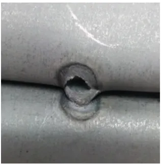
Figure 1.2 - The spot weld electrode at increasing stages of degradation, the notable surface

changes in the severely degraded cap are a result of material being lost from the cap

surface during welding. The rate at which caps degrade is highly dependent on the welding

conditions employed. ... 5

Figure 1.3 - An example of a peel test performed on a weld, the size of the welded area can

be measured from the fused region after completion. Although somewhat inaccurate, peel

testing is one of the fastest measurement methodologies... 7

Figure 1.4 - An example of a cross section after chemical etching, the austenitic growths

indicate that melting and subsequent solidification has occurred, allowing for a direct

measurement of nugget size to occur. ... 8

Figure 1.5 - The RSWA by Tessonics is an example of a post welding microscopy device.

Using a 52 element array the size of a weld is measured using signal processing techniques

(Tessonics, 2008). ... 9

Figure 1.6 -The RIWA monitoring system, consisting of a transducer within the water cooling

column and two or more metal sheets. This system allows for weld quality measurements

to occur in real-time with little modifications needed to the existing system. ... 11

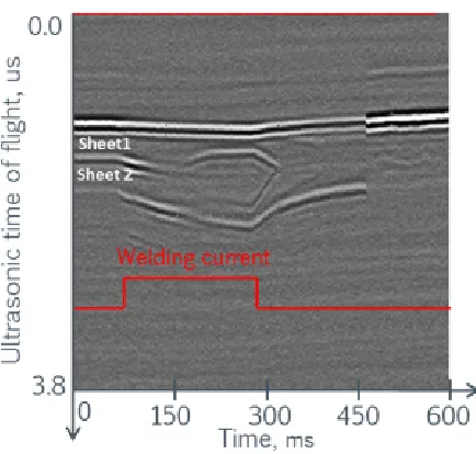
Figure 1.7 - The differing reflections between the unwelded and molten stages of the weld.

The transformation of the central reflection into two separate reflections is indicative of

melting occurring within the welding stack. ... 11

Figure 1.8 – An ideal M-scan, where the development of all boundaries is clearly visible

throughout the welding process. Although ideal, the variance between welding setups

(12)

xi Figure 1.9 - The functionality of the phased array scanning technique. Using phased array

imaging techniques, multiple cross sections can be acquired along the welded plates,

allowing for far more information than the current RIWA system. ... 13

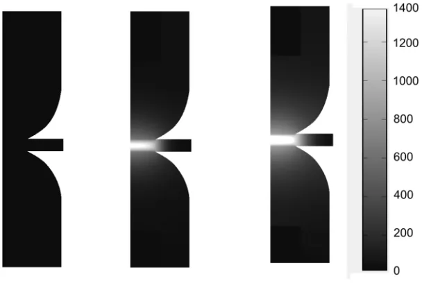
Figure 1.10 - Temperature distributions for the model at the beginning, middle, and end of

welding for a 8kA 20 cylce weld, by extracting the values for any given point in time. The

thermal gradients present in the system can be determined for arbitrary points in the

welding process. ... 15

Figure 2.1 - Contrast of the difference between the propagation of shear and longitudinal

waves. The particle location in each case is depicted by the intersection of the grid lines. It

should be noted that although the particle motion is different in each case the wave’s

direction of propagation remains unchanged. ... 19

Figure 2.2 – A graphical representation of the direction of wave propagation as it passed

through and is reflected from a boundary. Due to mode conversion a ray incident at angle

can produce both a longitudinal and shear wave propagating at angles and

respectively. ... 23

Figure 2.3 - A plot of the transmission coefficients and mode conversion between water and

copper for shear and longitudinal waves. In order to reduce mode conversion angles of less

than 17° should be employed. ... 24

Figure 2.4 - An example of a B-Scan on a media with a void present, any object or boundary

within the emitted ultrasound field(left) having its reflections detected and displayed in the

resulting image(right). ... 27

Figure 2.5 - An example acquisition of a B-scan. An A-scan is created by acquiring ultrasound

data at multiple scan locations and creating a figure corresponding to the spatial or

temporal locations at which these scans are acquired. ... 28

Figure 2.6 - The stark difference between the near and far field emission of a transducer. As

is seen, the near field has inherent oscillations in both spatial directions, while the far field

(13)

xii Figure 2.7 - A depiction of the electronic delays and emission fields of a phased array probe

for electronic steering (a and b) and electronic focusing (c and d) with and without steering

applied. It should be noted that near fields and far field variations exist for all cases. ... 31

Figure 2.8 – A diagram depicting the various parameters of the phased array. These

properties can be modified to maximize imaging abilities for specific situations. ... 32

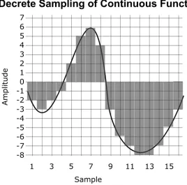
Figure 2.9 - A depiction of the sampling of a continuous waveform at discrete amplitudes

and time values, depicted using points and lines respectively. Improper discretization of

both the frequency and amplitude can result in large errors when reconstruction is

attempted. ... 34

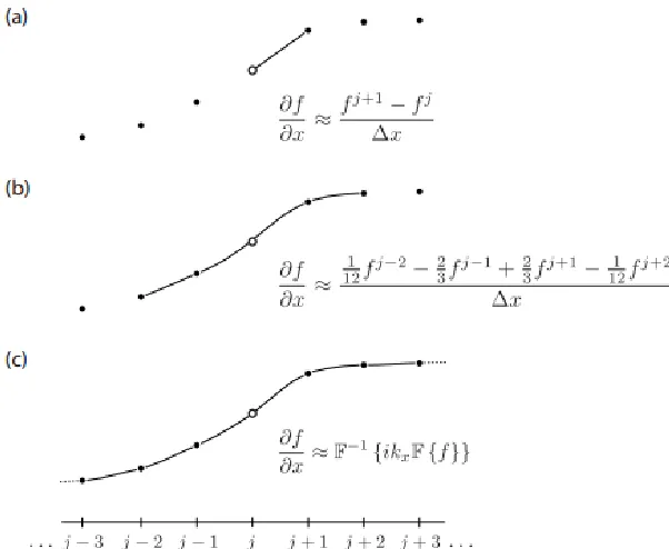
Figure 2.10 - A comparison of differing calculation techniques for spatial gradients using a)

first order forward difference, b) Fourth order central difference, c) Fourier collocation

spectral method 12_{. ... 37}

Figure 2.11 - An example of Gibbs ringing artifacts caused by high discontinuities within the

media. As can be seen, only the decay rate of the amplitude is modified through the

increase of the spectral sampling with the initial overshot remaining constant. ... 38

Figure 3.1 - The housing of the previous probe was designed to allow for water to be

supplied via external channels. A small plastic insert was used to electrically separate the

transducer from external currents, as well as prevent leaks. ... 43

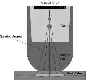
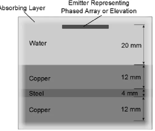
Figure 3.2 - The simulation environment, consisting of the three media within the system.

The geometry of the copper cap is ignored for simplification and perfect coupling assumed

between each media... 45

Figure 3.3 – A depiction of the array’s emission profile and its varying components. ... 46

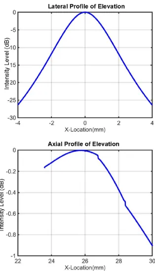
Figure 3.4 - The depiction of the amplitude distributions for the elevation of the previous

transducer. ... 48

Figure 3.5 - The depiction of the amplitude distributions for an on-center focus using the

(14)

xiii Figure 3.6 - The depiction of the amplitude distributions for an off-center focus using the

previous phased array design. ... 50

Figure 3.7 - An example of how a rectangular transducer can be used within a circular

housing to allow for cooling water to be incorporated into the design ... 51

Figure 3.8 - A comparison of the difference between the focused for varying elevation sizes.

... 55

Figure 3.9 – Simulated results for a 5 mm elevation, with a varying size of water column. .. 56

Figure 3.10 - The amplitude field profiles for an 8 mm active aperture with differing element

sizes for an on-center focus. ... 59

Figure 3.11 - The amplitude field profiles for an 8 mm active aperture with differing element

sizes for an off-center focus. ... 60

Figure 3.12 - The transducer housing design showing internal (2), external (1&3) designs and

the resulting product from top to bottom ... 62

Figure 3.13 - The response function of both the new and old transducer to a line spread

phantom. As is clearly seen the new transducer has a significantly higher focus than that of

the previous system. ... 66

Figure 3.14 - The line spread function of the copper phantom compared to its simulated

response in copper. The difference between the experimental and theoretical amplitudes

does not exceed 7%. ... 67

Figure 3.15 - The pulse duration of the signal after beamforming. A long duration of the

signal indicates a ringing of the transducer occurs after initial excitation. ... 68

Figure 3.16 - A measurement of the linearity of the new and old system measured from a

flat planar boundary. Both systems exhibit nonlinear intensities within the region of interest

... 69

Figure 4.1 - The temperature profile extracted at the end of welding using previous

(15)

xiv Figure 4.2 - The time difference between a thermally constant and thermally varying media.

The difference is notably proportional to both the heating along the trajectory and the

length of the trajectory. ... 74

Figure 4.3 - The phase delay difference associated with the time of flight difference, the

difference in the phase delay increases as the focal points move away from the center of

the media. ... 74

Figure 4.4 - The waves resulting from the summation of ideal point sources with the phase

delay offsets applied. The resulting waveforms indicate that at the edge of the imaging field

a reduction of 15% in amplitude would occur in a worst case scenario. It should be noted

that the temporal shift of the wave can be corrected for in post processing. ... 75

Figure 4.5 - The change in amplitude and position of the beam emission pattern, as

normalized to the pattern with no gradients present. ... 78

Figure 4.6 - The transmission coefficient between water and copper as a function of

temperature for a perpendicularly incident wave. As temperature increases a greater

portion of the incident wave in transmitted in the region of modeled temperatures ... 79

Figure 4.7 - The speed of sound ratio between water and copper as a function of

temperature. Through Snell’s law it can be noted that an increase in temperature will lower

the angle of transmission, resulting a wave whose final position is closer to the center of the

weld nugget. ... 79

Figure 4.8 - The speed of sound ratio between a copper/steel boundary as a function of

temperature. Very little change is indicated through the range in which copper is solid and

the transmission angle is dependent almost solely upon the incident angle. ... 80

Figure 4.9 - The transmission coefficient between copper and steel as a function of

temperature. The transmission coefficient is essentially unchanged over the temperature

range for which copper is solid. This indicates that any change in the reflected wave from

(16)

xv Figure 4.10 - The change in angle a wave will experience when intersecting a molten nugget.

The fact that the angle of transmission is roughly half that of incidence means that

reflections from inside of the molten pool may be affected during the early stages of molten

growth. ... 82

Figure 4.11 – A plot of data collected from the system prior to welding and the

corresponding noise. Although electrical noise was found to be negligible in the acquisition

process small shifts in the position of the transducer results in minor shifts to the boundary

position, introducing some variance in the reflections position within the image. ... 84

Figure 4.12 - A depiction of the time evolution of the copper steel boundary amplitude and

position. The amplitude of the reflection was found to significantly decrease as the steel

plates heated, eventually reaching a minimum. ... 85

Figure 4.13 - B-scan acquired at the end of solidification. At the end of heating a clear

curved appearance is present in the interfaces. This curvature is indicative of lower angle

trajectories being remapped to higher values, as the wave is expected to travel further than

they do. ... 88

Figure 4.14 - An amplitude profile along the final weld piece. The reflections from the edges

appear to be over predicted by approximately 0.5 mm on each edge. This indicates that the

modelled effects are occurring, however the error associated with measure means that

such conclusion is not definitive. ... 89

Figure 4.15 - A cross sectional view of the weld. Cross sectioning reveals that the final

location of the unbonded region is approximately 1.5 mm on both sides of the nugget. .... 89

Figure 4.16 - The acoustic microscope image of the weld. Scanning of this plate during

welding is taken at the Y-axes origin. Bonded area is estimated using the darkest region. A

high variance was found to result when compared to the cross sectioned image due to the

presence of a weak bond around the edge of the weld. ... 90

Figure 4.17 – A comparison of the extracted profile from each of the methods used.

(17)

xvi resolution difference and non-linearity of the imaging system have a large influence on

comparison results. ... 90

Figure 4.18 - The acquired B-scan prior to the start of welding. A small curvature towards

the edge of the image indicates that the geometric structure of the electrode has some

influence in these regions. ... 91

Figure 4.19 – The acquired B-scan at the end of welding. Although increased coupling has

resulting in a change in the copper-steel boundary amplitude no increase in the curvature of

the boundary is present. This indicates that the resulting thermal offsets have no notable

(18)

xvii

LIST OF APPENDICES

Appendix A – Total Focusing Matlab Code………96

Appendix B – Calculation of Trajectory though Two Boundary Media…………..99

Appendix C – Code for Calculation of Trajectory Through Layered Media…….100

(19)

1

Chapter 1 Introduction and Background Theory

1.1 Introduction

The spot weld process is a widely used technique in the sheet metal joining industry

and specifically in the automotive sector1_{. This technique makes use of resistive}

heating to fuse metal sheets together at a point. Although a common technique, the

use of new alloys and metals in an attempt to reduce vehicle weight has resulted in

alloys that are more difficult to weld and more likely to encounter issues.

The majority of these issues result from repeated use of the spot weld electrodes

causing deformation of the electrode surface, changing the welding conditions.

Although remedies such as polishing of the electrode cap to restore the original

surface are employed the electrode cap will eventually require replacement. Due to

the fact that the electrodes are water cooled, replacement of the caps requires that

automated assembly lines be shut down. The expense associated with this often

results in the need for balancing weld quality and minimizing downtime.

Due to this extended use of the electrodes, most companies employ some form of

testing on the performed welds. Although offline testing methods have been well

established, the time requirements means that only a small portion of the welds can

be tested. If severe issues are detected at this point an entire batch of welded parts

may be scraped2_{. For this reason it is highly desirable to monitor every weld that}

occurs in real time.

Although a variety of inline testing methods have been proposed to perform this

task3_{, one technique currently employed in an industrial environment makes use of}

an ultrasound transducer build into the spot weld electrode4_{. This method,}

(20)

2 ultrasound waves. By doing this repeatedly a quality signature of the weld can be

created and feedback can be given in real time5_{. Although this system works well in}

the majority of cases it allows for monitoring only along the center of the weld.

In order to alleviate this constraint a system was developed to allow for acquisition

along a cross section of the weld6_{, this system was shown to have some success, but}

was limited to imaging in laboratory conditions. In addition to these limitations the

effects of the temperature gradients produced as the sheets are heated was

considered negligible. Due to the large gradients produces during welding a

quantification of their effects on the imaging process was required to allow for

proper assessment of weld quality.

With these limitations in mind, this research was undertaken with two primary

goals. First a redesign of the system was needed to improve its imaging abilities and

allow for its use outside of laboratory conditions. Secondly the imaging abilities of

the system needed to be quantified and the effects of thermal gradients on these

imaging abilities determined.

1.2 Overview

This chapter covers the basic principles of welding and discusses the problems that

can arise during welding. It covers a method of ultrasonic monitoring that has been

developed for use within our group and is the basis for this research.

In Chapter 2 the basics of ultrasound propagation and ultrasound imaging are

discussed to familiarize the reader with concepts used in this work. It also introduces

the reader to the finite element modelling process employed in this work.

Chapter 3 investigates the limitations of the previously used system and the steps

taken to optimize its imaging abilities. It also covers the experimentally determined

(21)

3 Chapter 4 covers the effects that the thermal gradients produced during spot

welding will have on the imaging process. These effects include changes to both the

accuracy and resolution of the system as the weld develop.

Finally Chapter 5 summarizes the abilities and limitations of the system developed.

This chapter also summarizes the future potential of the system and the

improvements that can still be made.

1.3 The Spot Weld Process

The spot welding process, as outlined in figure 3.1, makes use of two or more metal

plates clamped between conductive electrodes, often constructed of copper. Large

forces, typically of between 500-1000 N, are applied to the sheets by the electrodes

to reduce the contact resistance at the point to be welded. The spot weld controller

then allows for the flow of a large current, typically 6000-22000 A in steel, to flow

through the metal sheets. This current results in resistive heating, eventually causing

melting to occur. At this point the current is turned off and the weld is allowed to

cool. Upon solidification the pool of molten metal fuses between the sheets

resulting in a joint that can have a comparable strength to the base materials7_{. In}

order to reduce the damage to the copper electrodes during this process and

increase the speed at which subsequent welds can be performed water cooling is

(22)

4 Figure 1.1 - A depiction of the spot weld process at the various stages, prior to welding, during welding and post welding. At the end of welding a fused region is

visible in the middle of the stack-up.

In this process, the heat generated within the metal stack is at times difficult to

predict due to the presence of multiple metals and the addition of coatings or oxides

on the surface of these materials. Although when considered in totality these effects

are difficult to describe the basic process is still governed by the underlying physics.

In this case the heating within the system occurs through the joule heating effect, as

described in equation 1.1, whereby the heat generated Q (in joules) is proportional

to the resistance of the metal R, measured in ohms, multiplied by the square of the

current, I, in amps and the time for which the current is applied t, measured in

seconds.

1.1

During this process, heat flows from the system primarily through basic thermal

conduction, described using equation 1.2 below. Whereby the heat flux q ⁄

is proportional to the conductivity of the material k(W/m/K) multiplied by the

change in temperature.

(23)

5

1.4 Quality Factors in the Spot Weld

The introduction of new metals and alloys in an effort to decrease vehicle weight

and increase fuel efficient has resulted in the use of materials that are difficult to

weld and prone to issues. One of the common causes of problems in the spot weld

process occurs due to the fact that the electrode caps are used for extended periods

of time. During their usage, heating of the copper, high forces and chemical

reactions at the surface between the metals results in a degradation of the surface

quality8_{. The degradation process is complex, but usually results in changes to the}

surface size, shape and structure of the cap8_{. This degradation, depicted in figure 2.3}

is highly dependent on the materials being welded and the selected welding

schedules.

This degradation results in a change in both the force and current distributions that

flow through the weld surface, causing a large change in the heating rates and the

heat distribution. Although some techniques such as polishing, where the surface of

the weld electrode is refinished, can be used to alleviate these effects, the caps will

eventually have to be replaced.

Figure 1.2 - The spot weld electrode at increasing stages of degradation, the notable surface changes in the severely degraded cap are a result of material being lost from the cap surface during welding. The rate at which caps degrade is highly dependent

(24)

6 If the surface area of the caps increases, current density and heating will decrease,

resulting in the weld size falling below the manufacturer specifications. In the limit

of low heating it is possible to generate welds in which incomplete fusion or no

fusion is present between the sheets. These are referred to as stick welds due to the

fact that elastic deformation of the metal forms weak bonds, causing the sheets to

stick together9_.

If deformation results in a decreased contact area more localized current densities

and higher heating will result. As the heat increases within the structure a variety of

metallurgical effects can occur, causing the formation of brittle structures within the

spot weld that will fail prematurely or in an undesired way. In the extreme internal

pressure can exceed the cohesive force of the molten pool. In this situation the

molten metal can be expelled from the pool, resulting in a decreased weld size and a

reduction in the thickness of the base metal9_{. Unlike undersized welds the effects of}

overheating and expulsion are harder to characterize. This is due to the fact that the

weld size is not the primary limitation in the strength of these welds and failure

points are more difficult to determine due to the randomness of expulsion nature.

Other problems that can occur in the spot weld process occur due to the metal used

in the process and the heating rate. Although a variety of problems exist the most

common are stress cracks and voids that form during the cooling process. Voids are

caused by gases becoming trapped within the molten pool, while cracks occur

mostly due to brittle alloy formation. Although more random in nature these

problems can often be found using current testing methods9_.

1.5 Monitoring Techniques

In order to assess the quality of a spot weld it is common to use monitoring

techniques throughout the manufacturing process. When employed frequently,

(25)

7 and allows for correction of the cause, preventing further issues. Monitoring

techniques can be separated into two distinct categories, those performed offline

and those performed in-line with the assembly process.

1.5.1 Offline Techniques

Offline techniques for monitoring any process often have a number of advantages

due to the fact that they are performed by trained inspectors and allow for the

correction of issues that may prevent a proper assessment of weld quality. Due to

the amount of existing techniques for offline monitoring, only the ones used in our

lab will be discussed, although more complete studies are available10_.

One of the most common techniques used to rapidly assess weld quality in the lab

environment is the peel test. In this test two sheets of metal are welded and the

weld is peeled back until failure occurs. Depending on the modality of failure and

resulting inspection the size of the weld nugget can be determined and the quality

of the weld can be assessed in a basic manner. An example of a peeled test sample

can be seen in figure 1.4 below, where the resulting weld has failed by tearing out of

the base material, allowing for a measure of its size using calipers.

Figure 1.3 - An example of a peel test performed on a weld, the size of the welded area can be measured from the fused region after completion. Although somewhat

(26)

8 If more information is desired as to the underlying metallurgical structure of the

spot weld it is common to perform cross sectioning of the weld sample. In cross

sectioning the weld is sliced in half and seated in a resin base. It is then polished to a

fine finish and etched in order to highlight varying structures (figure 1.5). By viewing

these structures under an optical microscope it is possible to estimate how heating

occurred within the weld and the resulting shape of the fused area. If chemical

composition is desired the samples can undergo further imaging using x-ray

diffraction.

Figure 1.4 - An example of a cross section after chemical etching, the austenitic growths indicate that melting and subsequent solidification has occurred, allowing

for a direct measurement of nugget size to occur.

Although these tests allow for a determination of the characteristics of the weld,

they require that the weld be destroyed in order to do so. As a result of this they are

impractical for testing on more than a select few welds. When welds require testing

without destruction non-destructive testing (NDT) are employed. Although a variety

of techniques can be used in NDT, ultrasound is one of the most widely employed

due to the fact that it allows for visualization of a subject in a safe and cost effective

(27)

9 One technique employed in many NDT applications is that of the scanning acoustic

microscope. Acoustic microscopy makes use of a higher resolution ultrasound

transducer and a mechanical stage to perform a raster scan of an object11_{. In order}

to accomplish this the part to be imaged must be submerged into a liquid bath to

allow for adequate sound transmission. In this method of imaging the region of

unfused metal can be imaged using a cross sectional scan. By measuring the region

in which no signal is detected from between the plates the total area of fusion can

be obtained12_{. Although this technique allows for very high resolution images to be}

obtained it suffers from the fact that the part being imaged must fit inside the limits

of the mechanical stage, often limiting this form of imaging to small parts or portions

of a work-piece. For this reason acoustic microscopy is not often used outside of lab

samples for weld measurements.

Adaptations of this technique have been implemented using a matrix array

transducer. By implementing an element by element scan it is possible to image a

region the size of a weld in a rapid manner. As before the welded area is determined

by the region in which fusion causes no reflection. An example of such a system is

features in figure 1.6 below10_.

Figure 1.5 - The RSWA by Tessonics is an example of a post welding microscopy device. Using a 52 element array the size of a weld is measured using signal

(28)

10

1.5.2 Inline Techniques

Although offline testing often yields high quality analysis of the weld it must be

performed by trained employees or professionals. In the highly automated

environments in which spot welding is used this requires an impractical time

investment, limiting the evaluative process to select samples. This selective process

means that problems can be undetected until after production has concluded,

resulting in a large amount of waste product being produced.

For this reason the need for a real time monitoring system is crucial. A real time

system can be considered as any system capable of assessing the weld quality in a

manner such that production is not significantly affected by its use. Many attempts

have been made to adapt offline systems into an automated environment10_{, but}

these systems tend to suffer alignment issues that make their use impractical. Other

methods such as monitoring the weld parameters such as voltage, current and

electrode displacement have proven to have some effectiveness10_{, but suffer from}

the fact that these parameters are material and setup specific and require

calibration in each case. Currently the most promising system for integration in a

welding environment is the real time inline spot weld analyzer (RIWA) 13_.

The RIWA system was developed within our research group at the University of

Windsor. It makes use of a transducer placed inside the water cooling of the

electrode to monitor the welding process as it occurs4_{, as in figure 1.7. This system}

works on the principle that the changes in the material that occur during the heating

process can be monitored and that direct inference can be made from this

knowledge6_{. In order to establish that a good weld has been performed the change}

from an unwelded to a welded reflection, seen in figure 1.8 is desired. In an ideal

condition the weld signature such as that obtained in figure 1.9 results. In this case

heating results in a change in the boundary position due to the corresponding

(29)

11 the plates splits into the reflection from the top and bottom of the molten pool.

These reflections change with respect to the size of the molten pool. After the end

of heating the weld begins to cool until the nugget has completely solidified,

resulting in reflections only from the top and bottom of the bounded structure.

Figure 1.6 -The RIWA monitoring system, consisting of a transducer within the water cooling column and two or more metal sheets. This system allows for weld quality measurements to occur in real-time with little modifications needed to the existing

system.

Figure 1.7 - The differing reflections between the unwelded and molten stages of the weld. The transformation of the central reflection into two separate reflections is

(30)

12 Figure 1.8 – An ideal M-scan, where the development of all boundaries is clearly

visible throughout the welding process. Although ideal, the variance between welding setups mean that not all boundaries may necessarily be visible in most

cases.

Although the RIWA system has been established as a solution to many problems and

is currently used in an industrial environment, the fact that it is limited to imaging

the central portion of a weld make its use impractical in some situations. In addition

to this the problems it can detect are limited to its region of view. This may not be

an issue in many areas, but can cause problems in situations where welds are

considered critical. A critical weld can be classified as a weldment whose quality

must be dependable for safety concerns. These welds are often limited to areas such

as seat belts, but can extend to many regions in the aviation industry. In these cases

the use of the RIWA system must often be accompanied by offline inspection.

In order to allow for imaging along more than one dimension the investigation of

using a phased array to image the spot weld process was done. Phased arrays,

discussed in the next chapter, allow for the use of multiple transducers to scan at

points within space. This technique, seen in figure 1.10 was shown to have the

(31)

13 a cross sectional analysis to be performed6_{. Although this device allowed for good}

estimations of the size of spot welds its imaging abilities were unknown and its use

was limited to laboratory conditions. This thesis covers the improvements made to

the initial design and investigates the limitations of the improved array.

Figure 1.9 - The functionality of the phased array scanning technique. Using phased array imaging techniques, multiple cross sections can be acquired along the welded

plates, allowing for far more information than the current RIWA system.

1.6 Spot Welding Model

The finite element model of the spot weld process used in this thesis was developed

and tested by a previous student in the group14_{. This model was based off of}

previously published work15_{and was performed using the COMSOL finite element}

modelling program. It relies on the use of a coupled electrical thermal model to

determine the temperature distributions in the spot weld system. In order to

decrease computational time axial symmetric model of the process was employed,

(32)

14 In this model the spot weld process is divided into discrete representation of the

system by selecting an appropriate spatial mesh. By separating the model into finite

steps in time the evolution of the welding model can be found. Using temperature

dependent material properties found in a materials product database it is possible

to describe the material over the range of temperatures for which welding occurs.

For each time step within the model the resistance at each node in the mesh is

found. This resistance can be used to calculate the current densities within the

model at this point in time. This current flow model is then used with the resistance

of the material to allow for the calculation of the heat generation at each point in

space. This generated heat is then allowed to propagate through the media for a

small amount of time. By starting from the initial welding conditions and slowly

repeating the previous processes an accurate model of an idealized spot weld can be

created.

In order to verify this model mesh refinement studies were conducted to ensure

accuracy in the predicted temperatures. Experimental validation was also performed

by extraction of the temperature profile at the axes of the weld. By comparing the

expected time of flight between each boundary to those achieved during

(33)

15 Figure 1.10 - Temperature distributions for the model at the beginning, middle, and end of welding for a 8kA 20 cylce weld, by extracting the values for any given point in

(34)

16

References

[1] N. T. Williams, J. D. Parker, Review of resistance spot welding of steel sheets Part

1 Modelling and control of weld nugget formation, International Materials

Reviews, Vol 49, No 2, DOI: 10.1179/095066004225010523, (2004).

[2] J. D. Cullen, N Athi, M. A. Al-Jader, A. Shaw, A. I. Al-Shamma’a. Energy Reduction

for the spot welding process in the automotive industry. Sensors and their

Applications XIV, Journal of Physics: Conference Series 76. (2007).

[3] S. Rivas, R. Servent, Tecnitest Ingenieros SL, Madrid, Spain;

J. Belda, Eines, Valencia, Spain. Automated Spot Weld Inspection in the

Automotive Industry. WCNDT-2004 Proceedings, Vol 10, No 3. (March 2005).

[4] Roman Gr. Maev, Andrei A. Ptchelintsev,John L. Mann , Transducer built into an

electrode US Patent No 6297467. (2001)

[5] Roman Gr. Maev, Andriy M. Chertov, John M. Paille, Frank J. Ewasyshyn,

Ultrasonic In-Process Monitoring And Feedback Of Resistance Spot Weld Quality.

US Patent No. 706940US1, (2013)

[6] Lui, Anthony, Development of an Ultrasonic Linear Phased Array System for

Real-time Quality Monitoring of Resistance Spot Welds. Electronic Theses and

Dissertations. Paper 4826. (2012)

[7] X sun. Failure Mechanisms of Advanced Welding Processes. Woodhead

Publishing Limited, (2010).

[8] Masatsune Kondo, Tokujiro Konishi , Koji Nomura & Hiroyuki Kokawa,

Degradation mechanism of electrode tip during alternate resistance spot welding

of zinc-coated galvannealed and uncoated steel sheets, Welding International,

(35)

17 [9] Hongyan Zhang, Jacek Senkara, Resistance Welding: Fundamentals and

Applications, (CRC Press, 2005).

[10] Runnemalm, A. and A. Appelgren, Evaluation of non-destructive testing methods

for automatic quality checking of spotwelds, in SpotLight, report No 13. (2012)

[11] R. Gr. Maev, Accousit Microscopy: Fundamentals and Applications, (Wiley,

2008).

[12]A. M. Chertov, R. G. Maev, and F. M. Severin, “Acoustic microscopy of internal

structure of resistance spot welds," IEEE Tran. on Ultrasonics, Ferroelectrics,

and Frequency Control, vol. 54, no. 8, pp. 1521-1539, (2007).

[13] Waldo J. Perez Regalado, Andriy M. Chertov, Roman Gr. Maev, Valdir

Furlanetto, Integration of the Ultrasonic Real-Time Spot Weld Monitoring

System, 5th Pan American Conference for NDT, (October 2011)

[14] Anthony C. Karloff, Real-time Expulsion Detection and Characterization in

Ultrasound M-scans of the Resistance Spot Welding Process, Electronic Theses

and Dissertations, Paper 4735, (2013).

[15]A. Karloff, A. Chertov, J. Kocimski, P. Kustron, and R. Maev, New developments

for in situ ultrasonic measurement of transient temperature distributions at the

tip of a copper resistance spot weld electrode, in Proc. IEEE Int. Ultrasonics Symp.

pp. 1424-1427. (2010)

[16] M. A. Al-Jader, J. D. Cullen, N. Athi and A. I. Al-Shamma'a. Experimental and

computer simulation results of the spot welding process using SORPAS software.

(36)

18

Chapter 2 Ultrasound Theory and Imaging

Ultrasound is a generic term used to describe any sound waves traveling above the

range of human hearing (20 kHz). Ultrasound has a wide range of applications in

both medical and industrial fields due to its ability to be used as a detection and

characterization tool. This chapter discusses the fundamentals of ultrasound and

ultrasound imaging necessary to understand the concepts explored later in this

work1_.

2.1 Ultrasound Principles

2.1.1 Sound Propagation

Sound waves are waves that propagate through media due to interactions between

the particles. Like all waves they have characteristic parameters such as frequency,

amplitude and phase. These parameters, in addition to the properties of a medium,

describe how this wave will propagate in space. Like all waves their motion is

described though the wave equation, expressed in both it’s coupled and decoupled

forms by equation 2.1 and 2.2a-c. Here p is the pressure, is the density of the

media, u is the particle displacement, is the speed of sound within the media and

t is the time2_.

1

0 2.1

! 1 2.2a

∙ ! 2.2b

(37)

19

2.1.2 Types of Sound Waves

There are multiple ways in which a sound waves can propagate, however for the

purposes of this work only two need to be considered. The simplest method of

propagation is that of the longitudinal wave, where collision of particles within the

medium generates regions of high and low particle density. Additional collisions

between the particles allow for the wave to propagate through the medium in the

same direction as particle motion. The second type of wave is that of the shear

wave. Shear waves are generated when a force is applied to the medium, such that

the internal particles are made to oscillate in some direction. The resulting wave

propagates within the medium through the bonding forces in a direction tangential

to the direction of particle movement. As a result of this propagation method shear

waves are often considered to only be supported within solid medium. A diagram

depicting these types of motion can be seen in figure 2.1.

Figure 2.1 - Contrast of the difference between the propagation of shear and longitudinal waves. The particle location in each case is depicted by the intersection

of the grid lines. It should be noted that although the particle motion is different in each case the wave’s direction of propagation remains unchanged.

Although both waves propagate in differing manner they can be expressed using

similar parameters, with the only notable difference occurring due to their varying

(38)

20 The speed of sound within both media can be determined using the elastic constants

of the material. The parameters necessary to determine the speed of sound are

Poisson’s Ratio, µ, Young’s Modulus, E, and the density of the media . This can be

done using equation1_{2. 3 and 2.4 for the longitudinal and shear velocity}

respectively.

# _{1 + μ 1 2μ}$ 1 μ 2.3

( #_{2 1 + μ}$

2.4

2.1.3 Refraction, Reflection and Transmission

For waves incident upon a boundary, the principles that govern the wave must

continue to hold, most notably its continuity and the total energy of the wave across

the boundary. In order for these principles to hold the wave must undergo a change

in its propagation direction and its amplitude. To determine the resulting change in

direction, Snell’s law is implemented. This well-known equation describes the

change in the waves propagation direction by a ratio of the sines of the incident and

transmitted waves angle, , with respect to the speed of sounds, c, as given by

equation 2.5.

)*+ ,

-.-

)*+ ,/

./

2.5

In addition to this change in the propagation angle of the wave, the amplitude of the

wave also undergoes a change described by the transmission and reflection

coefficient. These coefficients express the amount of the wave’s amplitude and

(39)

21 to the degree with which the impedances (equation 2.6) of the media differ. The

impedance of a medium, Z, is a parameter that couples the speed of a wave in the

medium, , with the density of the medium, .

0 2.6

The transmission (T) and reflection (R) intensity of the wave at the boundary can be

described by the magnitude of its velocity, pressure and intensity, relative to that of

the incident wave. In most instances the intensity or pressure coefficients are

chosen, as most ultrasound detection techniques are pressure based. The other

coefficients can be found through simple relations given in equations 2.7-2.10

below, with the corresponding subscripts for pressure (p), Intensity (I) and velocity

(u) used.

1 2 3

2 0₀4 3

2+ 1 2

2.7

2.8

2.9

2.10

The most basic case of reflection is that of a wave normally incident on the boundary

between two media. In this case the coefficients are expressible as a simple ratio of

impedances, given by equation 2.11 and 2.12 below. These relations also allow for

good approximation in cases of low angles of incidence.

2 0₀4 0

4+ 0

2.11

2 ₀20

4+ 0

2.12

In order to deal with a wave incident at an angle, additional considerations must be

addressed, mainly the fact that waves incident at angles can excite both shear and

(40)

22 all cases the waves propagate according to the underlying equations and changes in

propagation direction occur according to Snell’s law. Due to the variety of waves and

the fact that not all media support the propagation of shear waves, there are a wide

number of situations that can occur. These situations have been investigated

mathematically3_{however, a full consideration is not needed in most cases.}

In this thesis the primary source of mode conversion is the presence of the copper

water boundary in the system. For this reason a wave incident from a liquid media

and propagating into a solid must be considered. In order to determine the

reflection and transmission coefficients the densities of the media and speed of

sound for each type of wave must be known. In addition, the impedance of the

media is adjusted to account for angular propagation. This results in an intensity

transmission and reflection coefficient described by equations4_{2.13-2.15, where the}

angles are taken with respect to those in figure 2.2. Plots of the transmission

coefficients corresponding to the water-copper boundary can be seen in figure 2.3.

There are two regions of note, mainly the region of low incidence angle, and the

region after which the critical angle is encountered, when only shear waves are

transmitted into the media. In most system, due to the differing speed of sound

between shear and longitudinal waves effort is made to allow for the transmission of

only a single type of wave into the media. In these cases other modes of propagation

(41)

23 Figure 2.2 – A graphical representation of the direction of wave propagation as it

passed through and is reflected from a boundary. Due to mode conversion a ray incident at angle ₅ can produce both a longitudinal and shear wave propagating at

angles ₆ and ₇ respectively.

0 04

0 + 04

2.13

6 4206_{0 + 0}cos 2 7 4

2.14

7 4207_{0 + 0}cos 2 7 4

2.15

04 _{=>) ,};-<_?, 0 06cos 2 7 + 07sin 2 7 , 06 _{=>) ,};/<C_C

(42)

24 Figure 2.3 - A plot of the transmission coefficients and mode conversion between

water and copper for shear and longitudinal waves. In order to reduce mode conversion angles of less than 17° should be employed.

2.1.4 Attenuation of Sound Waves

During propagation through a medium a wave undergoes a variety of interactions

within the medium. These interactions generate a loss of the wave’s amplitude due

to scattering and absorption. Scattering is caused mainly due to the interaction of

propagating waves with the grain structure of the medium. At these grain

boundaries a high impedance mismatch exists, causing reflections of ultrasound

waves. Depending on the size of the grains, these reflections can have a significant

effect on the propagation amplitude and direction of the wave, causing losses to

occur. Absorption occurs due to the thermal interactions within the medium

converting sound to other forms of energy. These losses are often grouped together

into a term known as attenuation. The attenuation of a medium is best

characterized by the use of an exponential decay. In this case, as the wave

(43)

25 the wave E , an attenuation factor F ( G4) and the distance of propagation d in

units of cm.

E E ∗ eGJK _2.16

As imaging commonly relies on the use of broad frequency ranges, the frequency

dependence of attenuation must be considered. In this case the attenuation within a

media is best described by a power law attenuation factor, whereby the attenuation

coefficient F is expressed in terms of the frequency of the ultrasound wave, L, and a

power exponent factor1M_.

F F LN _2.17

This power law attenuation results in an uneven attenuation and a loss in resolution

as the wave propagates and higher frequencies undergo greater attenuation.

2.1.5 Intensity and the decibel scale

When imaging multiple media, a wide variation in the reflection amplitude of the

wave may be present, meaning that imaging often occurs at a wide range of

amplitudes. For this reason it is common to express the ultrasound signal on a

decibel scale. As ultrasound is measured on a pressure scale the intensity level, L, in

decibels can be calculated by relating the amplitude of a wave, A, to a reference

amplitude E through equation 2.18. The most common points of reference in the

decibel scale are the -6dB and -12dB points, corresponding to the loss of 50% and

90% of the compared amplitude.

20dB ∗ log₄ _EE 2.18

2.2 Principles of Ultrasound Imaging

Ultrasound imaging like all wave based imaging modalities relies on the principle

that a wave undergoes varying changes as it propagates through a medium. By

(44)

26 imaging two imaging modalities are primarily used, notably reflection and

transmission based imaging. In order to generate ultrasound waves the use of a

transducer is employed to convert electrical impulses to acoustic impulses.

In transmission based imaging waves are sent through the medium to a secondary

transducer. This yields only information about the loss in signal and relies on

comparison to a reference sample or samples acquired at other spatial or temporal

locations for assessment. Although this modality has been previously researched for

this work by others5_{it was rejected in favor of reflection imaging, and will thusly not}

be considered further.

Reflection images are based upon the use of a single transducer that acts as both the

transmitter and receiver of ultrasound waves. In this imaging modality a short

impulse is sent into the system and the reflections generated from the medium are

analyzed in order to allow for the determination of the medium properties. The

basics of this process can be seen in figure 2.4, where an amplitude scan or A-scan

allows for the determination of the amplitude and time between received

reflections. If the speed of sound is known this allows for the determination of an

(45)

27 Figure 2.4 - An example of a B-Scan on a media with a void present, any object or boundary within the emitted ultrasound field(left) having its reflections detected and

displayed in the resulting image(right).

Although the A-scan allows for the acquisition of information in the direction of

wave propagation it is often desirable to acquire information in more than one

dimension. In order to do this multiple A-scans can be acquired at differing spatial or

temporal locations by translating or rotating the transducer. By representing these

scans as an image and correlating amplitude to brightness a B-scan is generated

(figure 2.5). As the B-scan terminology can be used for many imaging modalities,

within this work it shall be reserved for describing spatially varying images. The

moving scan (M-scan) imaging modality will be used to describe B-scans whose

(46)

28 Figure 2.5 - An example acquisition of a B-scan. An A-scan is created by acquiring ultrasound data at multiple scan locations and creating a figure corresponding to the

spatial or temporal locations at which these scans are acquired.

All imaging modalities rely on the determination of the properties of the system, but

in most cases the introduction of undesired image artifacts occurs due to noise in

the system. One of the most common sources of error in ultrasound imaging is due

to the fact that the receiver and source of ultrasound do not transmit ideal waves

for imaging purposes. As the wave propagates, any objects which do not completely

block its path act as additional sources of reflection. This means that for waves with

large spatial distributions many reflections result from objects outside of the desired

imaging region. In order to prevent this, a transducer must be chosen such that the

emitted fields allow for coherent images to be acquired.

2.3 Transducer Selection

During transducer selection the primary parameters that control the imaging

process are the size, shape, frequency and pulse duration or bandwidth of the

transducer. The frequency of a transducer is the primary factor in determining its

resolution. During ultrasound imaging the fields emitted from a transducer result in

(47)

29 such a way that the amplitude is minimized outside of the imaging region it is

possible to generate high quality images. The design of an ultrasound probe is often

done to allow for a needed resolution to be obtained, while not incurring

unnecessary burdens that result from very high resolution systems.

In order to control the fields that are emitted from a transducer the size, shape and

frequency of the transducer can be modified. For the purpose of imaging the

emitted field of a transducer is separated into two distinct regions, the near field

and the far field. In the near field constructive and destructive interference result in

a widely varying intensity, with regions of null intensity, while in the far field the

intensity decrease proportionally to the distance. These field patterns are

characterized in figure7_{2.6 below.}

Figure 2.6 - The stark difference between the near and far field emission of a transducer. As is seen, the near field has inherent oscillations in both spatial directions, while the far field is expressed with a far more constant decay of the

wave’s amplitude

Due to the variability of the wave in the near field, this region is often undesirable

for imaging purposes, as any defects can be missed during examination. As the

amplitude is constantly decaying in the far field the last maximum occurs at the

boundary between the two. This boundary is referred to as the natural focus of the

(48)

30 can be found using the near field equation7_,_{where the near field distance N is}

proportional to the diameter of the transducer D and its wavelength within the

chosen imaging medium S. This allows for the calculation of the required transducer

size for a given imaging situation. In cases where multiple media are present the

near field is often modified using the small angle approximation. In this case the

diameter can be found using the depth of each media and their corresponding

wavelengths.

T U_4S 2.19

W4S4+ W S U₄ 2.20

By changing the shape of the transducer or employing an ultrasonic lens this focal

distance can be decreased by altering the interference pattern. Although this allows

for higher resolution at the focal point, the more rapid convergence and divergence

of the spatial distribution results in a decrease in the focal length of the system,

reducing the range of depth over which the beam remains focused and imaging can

occur.

In order to quantify the resolution of the system a common point of measure is the

-6dB. This point is chosen due to the fact that it corresponds to the full width half

max of the pressure emitted and describes the spatial resolution of the system. The

-20db location of the system is also given in some situations as additional reference.

The temporal resolution of a transducer is determined by the pulse duration,

defined as the period of time over which the wave’s enveloped amplitude decays,

again specified using the -6db measure of the wave. The pulse duration of a probe is

primarily influenced by the design process and methods used to manufacture the

(49)

31

2.4 Principle of Superposition and Phased Array Imaging

One of the primary problems with traditional imaging modalities is that the time

required to translate or rotate the transducer makes imaging some processes

impossible or impractical. In order to overcome this the use of phased array imaging

is employed.

Phased array imaging makes use of Huygens’ principle of superposition, which states

that any source of ultrasound can be broken down into individual point sources of

ultrasound, as long as the point sources are separated by less than the Nyquist limit

of the wave8_{. Phased arrays make use of the principle by dividing an ultrasound}

transducer into sub elements. By choosing the active elements it is possible to vary

the size of the active emitter and it’s corresponding field patterns. In addition to this

it is common to employ electronic delays to each element to further manipulate the

emitted fields, as shown in figure 2.7. These delays, known as focal laws, are chosen

such that the waves emitted from each element arrive in phase with each other and

are directly proportional to the difference in time of flight between each element

and the focal point.

Figure 2.7 - A depiction of the electronic delays and emission fields of a phased array probe for electronic steering (a and b) and electronic focusing (c and d) with and without steering applied. It should be noted that near fields and far field variations

(50)

32 During the design process the array parameters must be considered to allow for

optimal imaging. When sizing the array, the number of array elements, pitch

(spacing between the center of the elements) and the inter element spacing (size of

the cuts used to section the transducer into sub elements) can be varied to allow for

a variety of imaging situations. These parameters, summarized in figure 2.8 below

can be modified to optimize the array for specific applications.

Figure 2.8 – A diagram depicting the various parameters of the phased array. These properties can be modified to maximize imaging abilities for specific situations.

As phased arrays rely on the use of superposition to optimally focus, the array

elements must be chosen such that the Nyquist sampling criteria is met, mainly the

elements are sized such that they are less than half the size of the emitted sound

wavelength. If this condition is not satisfied imaging artifacts can occur due to the

presence of additional lobes in the emitted fields.

2.5 Ultrasound Acquisition System

In order to acquire ultrasound data an ultrasound acquisition system must be used.

These systems often consist of multiple components and subsystems depending on

the application they are to be used for. In the simplest case an ultrasound system

consists of a pulsar and receiver board along with control electronics and a

(51)

33 Pulsar boards consist of one or more pulse generator units. Simple pulsar boards

allow for the use or a unipolar or bipolar impulse to drive the ultrasound transducer.

Although more complex systems allow for arbitrary waveforms to be generated they

are rarely used in industrial applications due to their lower energy limit. Pulsar

boards allow for the control of the input pulse waveform at selected voltages and

emission windows. As the input pulse controls the emitted ultrasound wave the

board should be capable of generating impulses of between one quarter and one

half wavelength of the transducer frequency, as these are the typical emission

lengths chosen to optimize signal quality. If phased array imaging is to be used the

use of multiple pulsar boards can be employed alongside delay electronics to vary

emission patterns.

In order to acquire ultrasound signal the use of an ADC (analogue digital converter)

is coupled with amplification electronics. Any pressure incident on the transducer

will cause a voltage to be present across the ADC channel. Amplification is

performed before the data is sampled in order to allow for acceptable voltage levels

to be present for conversion. The two most important parameters of the ADC board

are its sampling rate and digitization ability. In order to acquire the signal, samples

must be taken at a chosen sampling rate, typically 50-100MHZ for phased array

systems. For each data point the amplitude is discretized into an amplitude value in

bits. For any ultrasound system the sampling rate must be chosen such that both the

desired frequency can be can be expressed and the amplitude is not saturated.

Amplifiers must be chosen such that the produced noise does not affect signal

(52)

34 Figure 2.9 - A depiction of the sampling of a continuous waveform at discrete amplitudes and time values, depicted using points and lines respectively. Improper

discretization of both the frequency and amplitude can result in large errors when reconstruction is attempted.

These two boards are coupled together with electronics that allow for rapid transfer

between the emission and reception boards, allowing a transducer that has been

used to emit the signal to sample immediately after. In order to reduce the cost of

the system it is common to use multiplexers to select active elements. This allows

for an arbitrary choice of elements for emission and reception of ultrasound data as

long as the number of chosen elements does not exceed the capabilities of the

system.

The rest of the ultrasound system is often less well defined, but contains the

electronics necessary for the storage and processing of the received data, as well as