New Results in the Linear Cryptanalysis of DES
Igor Semaev
Department of Informatics University of Bergen, Norway
e-mail: [email protected] phone: (+47)55584279
fax: (+47)55584199 May 23, 2014
Abstract
Two open problems on using Matsui’s Algorithm 2 with multiple linear approxi-mations posed earlier by Biryukov, De Canni`ere and M. Quisquater at Crypto’04 are solved in the present paper. That improves the linear cryptanalysis of 16-round DES reported by Matsui at Crypto’94.
keywords: linear cryptanalysis, multiple linear approximations, success probability, MRHS linear equations, gluing algorithm.
1
Introduction
Linear Cryptanalysis is one of the major techniques in the cryptanalysis of symmetric ci-phers. It was introduced and then improved in [10, 11] as an attack to DES by Matsui, though some similar ideas appeared independently in [9] as well. Linear Cryptanalysis is a known plain-text attack and it exploits that certain linear combinations, called ap-proximations, modulo 2 of the plaint-text, cipher-text and key bits are zeros with some a priori computed probability. Two attacks Algorithm 1 and Algorithm 2 were suggested in [10]. Algorithm 1 uses n-round approximations to attack n-round cipher, while Algo-rithm 2 usesn−1 or n−2-round approximations. The latter requires a lower amount of plain-text/cipher-text pairs and is more efficient.
For 16-round DES, Matsui shows how to determine candidates for key bits or key-bit linear combinations by Algorithm 2 with 243 plain-text/cipher-text blocks and success probability 0.85, then 243trials are run to get the correct key [11]. Two 14-round approx-imations considered statistically independent were there used together. How to improve Algorithm 1 with more than two approximations was shown in [7]. In [1] a framework for using many approximations considered statistically independent was proposed, though no practical cryptanalysis was presented. Two open problems related to Algorithm 2 were there posed. First, how to merge data from different approximations efficiently. Second, how to compute the success probability as a function in the number of available plain-texts and the number of trials in the search phase.
In the present note a solution to those problems is suggested. It is very different from the theory in [5]. The method or its straightforward generalisations are applicable to any cipher. In particular, for 16-round DES we show how by using 243 plain-text/cipher-text blocks and with at most 243trials in the search phase achieve the success probability 0.8925 with 10 approximations from 14-round DES. Overall running time is essentially 243 DES encryptions. Each of the approximations has at most 19 effective key bits(at most 18-bit subkey and a linear combination of the key bits), so the space amount is negligible. The cryptanalysis is easily implementable and practical.
Using more approximations increases the success probability further. For instance, with the first 24 best approximations it becomes 0.9006, though some approximations may have up to 43 effective key bits and the space requirement is heavy.
For 8-round DES the calculations were checked by experiments. 105 random keys were
generated, for each of them 1.49×217, as in [11], random plain-text blocks were encrypted with 8-round DES. For 243trials in the search phase, the empirical success probability was 0.8933(0.8925 in theory again) with 10 approximation from 6-round DES, each with at most 19 effective key bits.
2
Notation
LetY be a bit string of some length, then denote
Y{i, j, .., k} = Y[i]⊕Y[j]⊕..⊕Y[k], Y[i, j, .., k] = [Y[i], Y[j], .., Y[k] ].
LetYi, Yj, .., Yk be bit strings of the same length then
Y{i,j,..,k}[r] =Yi[r]⊕Yj[r]⊕..⊕Yk[r].
wherei= 1, ..,63 andi6= 0 mod 8. According to [10], any 14-round linear approximation implies
Φi(Di, Ki) =li(K) (1)
with probability pi for some explicit function Φi, where li(K) is a linear function in 56 variables K, the cipher key bits,Di are some plain-text, cipher-text bits andKi is a sub-key. The |Ki|+ 1 bits Ki, li(K) are called effective key bits for the approximation (1). Remark that in [10] onlyKi are called effective. LetXi−1, Xi denote the input to the i-th round andXi+1, Xi denote the i-th round output. So X0, X1 and X17, X16 are plain-text
and cipher-text blocks respectively, where the initial permutation is ignored. Let Kj be 48-bit round key at roundj. Then
X0{7,18,24} ⊕X17{15} ⊕X16{7,18,24,29} ⊕ F1(X1, K1){7,18,24} ⊕F16(X16, K16){15}
= K{3,5,7,9,11,13,15}[22]⊕K{4,8,12}[44] (2)
holds with probability 12− 78125
137438953472 = 1/2−5.6843×10
−7. That is the largest possible
in absolute value bias over all approximations with at most one active S-box in rounds 2,3, . . . ,15, see equation (33) in [10]. So Φ1(D1, K1) =l1(K), where
D1 = X0{7,18,24} ⊕X17{15} ⊕X16{7,18,24,29}, X1[11, ..,16], X16[27, ..,31,0], K1 = K[3,4,18,22,25,28,37,39,42,54,57,59],
l1(K) = K{4,7,13,14,39,45,46,49,50,59}. (2) is listed first in Table 7 as well.
3
Constructing and solving MRHS linear equations
3.1 Critical regions and error probabilities
Letn be the number of plain-texts andν =ν(a) denote the number of plain-texts, where Φi(Di, a) = 0. Letpi< 12. As the keyK is fixed, there are two possibilities forli(K).
First, assumeli(K) = 0. By (1) we have Pr(Φi(Di, Ki) = 0) =pi for correct Ki. One rejectsKi =aif
ν(a) n ≥
1 2 +xi,
otherwise Ki =ais accepted. We compute the probability of rejecting Ki =a under the condition that was correct and then wrong.
βi =Pr(rejectKi=a|correctKi =aandli(K) = 0) =Pr(ν/n≥1/2 +xi|pi).
That is the probability the normalised number of successes in Bernoulli trials with success probabilitypi is at least 1/2 +xi. So
βi=Pr
ν−npi √
npiqi ≥ √
n1/2√−pi+xi piqi |pi
≈Pr
N(0,1)≥√n1/2√−pi+xi piqi
(3)
by de Moivre-Laplace theorem [3], whereqi = 1−pi andN(0,1) denotes a standard normal random variable. Then
αi =Pr(rejectKi =a|wrongKi=aandli(K) = 0) =Pr(ν/n≥1/2 +xi|1/2). That is the probability the normalised number of successes in Bernoulli trials with success probability 1/2 is at least 1/2 +xi. Then
αi=Pr
ν−n/2
p
n/4 ≥2
√
n xi|1/2
!
≈Pr N(0,1)≥2√n xi
. (4)
Assume li(K) = 1 now, then Pr(Φi(Di, Ki) = 0) =qi for correct Ki. One rejects Ki =a if
ν(a) n ≤
1 2 −xi, otherwise Ki=ais accepted. Similarly
βi =Pr(rejectKi =a|correctKi =aandli(K) = 1)≈Pr
N(0,1)≥√n1/2√−pi+xi piqi
,
and
are true again. Therefore forpi <1/2 in both cases
βi ≈Pr
N(0,1)≥√n1/2√−pi+xi piqi
, αi ≈Pr N(0,1)≥2 √
n xi
. (5)
Letpi >1/2, then the critical region is ν(na) ≤ 12 −xi forli(K) = 0 and ν(na) ≥ 12 +xi for li(K) = 1. Therefore for p
i >1/2 in both cases
βi ≈Pr
N(0,1)≥√n1/2√−qi+xi piqi
, αi≈Pr N(0,1)≥2 √
n xi
. (6)
We summarise the criterion in Table 1.
Table 1: The criterion
li(K) pi rejectKi=aif 0 <1/2 ν(a)≥(1/2 +xi)n 1 >1/2 ν(a)≥(1/2 +xi)n 0 >1/2 ν(a)≤(1/2−xi)n 1 <1/2 ν(a)≤(1/2−xi)n
3.2 Collecting MRHS linear equations
Assume li(K) = 0 and let a01, . . . , a0s be the accepted values for Ki. Assume li(K) = 1 and leta11, . . . , a1tbe the accepted values for Ki. One writes this fact as
Ki li(K) =
a01 . . . a0s a11 . . . a1t 0 . . . 0 1 . . . 1
, (7)
where the columns on the right hand side are acceptable values for K i
li(K) . Thus a MRHS linear equation is constructed, see definitions in [13]. For eitherli(K) = 0 orli(K) = 1 the probability thatKi=ais (1−αi). Any|Ki|+ 1-bit string is in the right hand side of (7) with probability (1−αi). Hence the equation (7) has (1−αi)2|K
i|+1
right hand sides on the
average. The probability the correct value for K i
3.3 Solving MRHS linear equations
Though there are several methods to solve MRHS linear equations in [13], we use Gluing Algorithm. The Algorithm starts with (7) ati= 1. Formally, at each step a new MRHS linear equation
MiK= [ci,1, . . . , ci,si], (8)
is constructed, where Mi is a matrix of size ri × |K| of full rank and where ci,1, . . . , ci,si areri-bit strings. (8) is a gluing of the previous equation
Mi−1K =
ci−1,1, . . . , ci−1,si−1
and (7) for i = 2, . . . , N. In fact, the method is implementable as a walk over a search tree: the currentci−1,j1 is sought to be extended to some ci,j2 with a table look up and few
Xor’s, see Section 6.
As the right hand sides of the initial equations (7) are generated independently, a particularcappears in the right hand side of (8) with probabilityQi
j=1(1−αj) by Lemma 1,
Section 6. Thereforesi= 2riQi
j=1(1−αj) on the average. The complexity of constructing
the final equation (8), that is fori=N, is proportional to
s1+s2+. . .+sN = 2r1(1−α1) + 2r2(1−α1)(1−α2) +. . .+ 2rN N
Y
i=1
(1−αi) (9)
Xor’s of bit strings of various length, see (15) in Section 6. One then solves the linear systemMNK =c for each generatedc to find key candidates to brute force. The number of the key candidates is 2|K|QN
i=1(1−αi) on the average. 3.4 Success probability
To brute force 2|K|−t key candidates, there should be
N
Y
i=1
(1−αi) = 2−t. (10)
The success probability is
1−β= N
Y
i=1
(1−βi). (11)
By choosing critical regions, that isx1, . . . , xN, (11) is maximised under (10). We do not
4
16-round DES with 10 approximations
Let n= 243 and we want to brute force at most 243 key candidates. One takes 10 linear approximations (1) with the best biases listed in the rows I = [1, ..,7,10,11,24] of Table 7, each with at most 19 effective key bits. For each approximation (1), that is by using 10 counters as in [10], the frequencies λA of Di = A over all available plain-text/cipher-text blocks are collected. The cost per one plain-plain-text/cipher-text is negligible in comparison with one 16-round DES encryption. Then
ν(a) =X A
λA(1⊕Φi(A, a)), (12)
where ais mostly Xor’ed to A by the DES round function construction. So Fast Fourier Transform is used to compute the convolution (12) in time|Ki|2|Ki|+1 for all values ofKi as in [2] and for each of those approximations.
By searching α = [αi, i ∈ I] such that Q
i∈I(1−αi) = 2−13, the success probability
Q
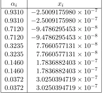
i∈I(1−βi) is maximised to 0.8925 at αi and xi shown in Table 2. Table 3 presents the
Table 2: 16-round DES, probabilities αi and critical region constantsxi
αi xi
0.9310 −2.5009175980×10⁻⁷ 0.9310 −2.5009175980×10⁻⁷
0.7120 −9.4786295453×10⁻⁸ 0.7120 −9.4786295453×10⁻⁸ 0.3235 7.7660577131×10⁻⁸
0.3235 7.7660577131×10⁻⁸ 0.1460 1.7836882403×10⁻⁷ 0.1460 1.7836882403×10⁻⁷
0.0372 3.0250394719×10⁻⁷ 0.0372 3.0250394719×10⁻⁷
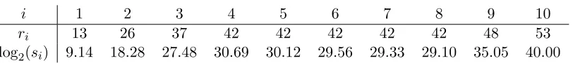
growth of the rankri and the number of right hand sidessi in the equations (8) produced by the Gluing Algorithm. The complexity of the Gluing Algorithm is at most 240of 17-bit Xor’s by (15). One does not need essentially more memory than to keep initial equations (7) as the algorithm is implementable, after some precomputation, with a search tree, see [14] and Section 6. As a right hand side c of the final equation is produced, one finds 256−r10 = 8 key candidates, solutions to M
10K = c, to brute force. The matrix M10 is
almost diagonal except one row contains two non-zero entries. So eachc specifies key bits ki for
Table 3: Gluing Algorithm complexity
i 1 2 3 4 5 6 7 8 9 10
ri 13 26 37 42 42 42 42 42 48 53 log2(si) 9.14 18.28 27.48 30.69 30.12 29.56 29.33 29.10 35.05 40.00
35,36,37,38,39,41,42,43,44,45,46,47,49,50,51,52,53,54,55,57,58,59,60,62,63}
andk23⊕k61. That makes 243trials on the average for all right hand sides together during
the search phase.
5
8-round DES experiments with 10 approximations
In this Section the results of the experiments on 8-round DES are reported. Let n = 1.49×217 and we want to brute force at most 243 key candidates. One takes 10 linear
approximations (1) with the best biases listed in the rows I = [1, ..,7,10,11,24] of Table 6, where 1-round approximations are from Table 5. By searchingα= [αi, i∈I] such that
Q
i∈I(1−αi) = 2−13, one maximises the success probability Qi∈I(1−βi) to 0.8925 at αi andxi shown in Table 4. The correctK is rejected ifν(Ki) is in the critical region defined byli(K), pi, xi for at least one i.
For each of 105 random 56-bit keys K, n random plain-texts were generated and
en-crypted with 8-round DES. The frequency of ”the correct K is accepted”, i.e. empirical success probability, was 0.8933. That is very close to the success probability computed theoretically.
6
Gluing Algorithm
Let
A1X= [B1], A2X = [B2] (13)
be a system of two MRHS linear equations, whereXis a column vector of unknowns,A1, A2
are matrices of full rank, that is no linearly dependent rows, with v1, v2 rows respectively.
Let B1, B2 be matrices whose columns are possible right-hand sides for AiX. Therefore X = x is a solution to (13) if the columns A1x, A2x belong to the columns of B1, B2
respectively. Letui be the number of columns in Bi.
Table 4: 8 round DES, probabilities αi and critical region constantsxi
αi xi
0.9300 −1.6699273321×10⁻³ 0.9300 −1.6699273321×10⁻³ 0.7150 −6.4277918792×10⁻⁴ 0.7150 −6.4277918792×10⁻⁴ 0.3255 5.1174922072×10⁻⁴ 0.3255 5.1174922072×10⁻⁴
0.1470 1.1871782307×10⁻³ 0.1470 1.1871782307×10⁻³ 0.0369 2.0217334996×10⁻³
0.0369 2.0217334996×10⁻³
1. Triangulate the concatenation ofA1, A2 by a linear transformU and get:
M =U
A1 A2
=
A1 U1A1+U2A2
, U =
E 0 U1 U2
,
whereE is an identity matrix. Then
¯ B1 =U
B1
0
=
B1 U1B1
, B¯2 =U
0 B2
=
0 U2B2
.
2. Letc1, c2 be columns of ¯B1,B¯2 respectively. Then c1⊕c2 defines a right hand side
toM X if and only if c1, c2 coincide on the entries, where M has a zero row. Let s
be the number of resulting possible right hand sides toM X.
3. M,B¯1,B¯2 are found, M X = [L] is constructed by u1 look ups andsof v2-bit Xor’s.
Assume now a system
A1X = [B1], A2X= [B2], . . . , ANX = [BN], (14)
whereAi are of full rank. Starting with the first equation, one constructsMiX = [Li] (i= 1, . . . , N) by gluing of Mi−1X = [Li−1] and AiX = [Bi]. As all linear algebra steps
may be precomputed, the algorithm reduces to look ups and vector Xor’s, see below. The constructing of the columns Li is implementable recursively with a search tree and therefore one only keeps the initial equations (14) after the precomputation and the current column at each step. Finally, the system solutions are the solutions toMNX = [LN]. The complexity isPN
We consider the algorithm in detail. Let vi be the number of rows in Ai and ui the number of columns inBi.
Precomputation. Initially, M1 = A1 is already triangulated and let ¯B1 = B1. For
i = 2, . . . , N the matrix
Mi−1 Ai
is triangulated by computing a matrix Mi of size
(Pi
t=1vt)× |X|:
Mi = U
Mi−1 Ai
=
Mi−1 U1Mi−1+U2Ai
,
U =
E 0 U1 U2
,
whereE is an identity matrix. Then matrices ¯Bj of size (Pi
t=1vt)×uj forj= 1, . . . , iare
computed by
¯
Bj ← U
¯ Bj 0 = ¯ Bj U1Bj¯
, j= 1, . . . , i−1,
¯
Bi = U
0 Bi = 0 U2Bi
.
The precomputation is finished.
Let bj be a column in ¯Bj, j = 1, . . . , i. Then ci =b1 ⊕. . .⊕bi, after reducing to the firstPi
j=1vj entries, is a correct right hand side forMiX if and only if the entries ofci in
the positions, where Mi has a zero row, are zeros.
So givenci−1 =b1⊕. . .⊕bi−1, one looks upbi such thatci−1, bi coincide on the entries in the positionsPi−1
t=1vt+ 1, . . . ,
Pi
t=1vt, whereMihas zero rows. The first
Pi−1
j=1vj entries
ofbi are zeros, so ci =ci−1⊕bi is computed withPNj=ivj-bit Xor’s. Letsi be the number
of the right hand sides toMiX, then the complexity of the algorithm is at most
N X i=1 si( N X
j=i
vj) (15)
bit Xor’s andPN−1
i=1 si look ups.
Example. LetX = (x1, x2, x3, x4) and there are three equations:
1 0 1 0
0 1 0 1
X = 0 1 0 1 ,
1 1 1 0
0 0 0 1
X= 1 0 0 0 ,
1 0 0 1
0 0 1 1
After precomputation M =
1 0 1 0
0 1 0 1
0 0 0 1
0 0 0 0
0 0 1 0
0 0 0 0
, B¯1 =
0 1 0 1 0 0 0 0 0 1 0 1
, B¯2=
0 0 0 0 1 0 1 0 1 0 0 0 ¯ B3 =
0 0 0 0 0 0 0 0 0 0 0 1 .
One is to combine columns bi in ¯Bi such that c2 =b1⊕b2 has zero in the position 4 and c3=c2⊕b3 has zero in the position 6. So the final MRHS linear equation is
1 0 1 0
0 1 0 1
0 0 0 1
0 0 0 0
0 0 1 0
0 0 0 0
X= 0 1 0 1 0 0 0 0 0 1 0 0
and the solutions are X = (0,0,0,0),(0,1,1,0). There is a better way to solve those particular equations. Each of them is equivalent to an ordinary linear equation:
1 1 1 1
X= 0, 0 0 0 1
X = 0, 1 0 0 1
X = 0,
see [13] for detail. The solution follows.
Lemma 1 Let M X = [L] be a gluing of AiX = [Bi], i= 1, . . . , N and γi, γ be the prob-ability a particular bit-string is a column in Bi, L respectively. Assume the columns in Bi
are independently chosen, then
γ= N
Y
i=1 γi.
Proof. Each column inLis determined by a column from each ofBi. Vice versa, a column inLdetermines those columns in Bi uniquely. That implies the lemma.
References
[1] A. Biryukov, C. De Canni`ere, and M. Quisquater,On Multiple Linear Approximations,
in CRYPTO’04(M.Franklin ed.), LNCS vol. 3152, Springer, 2004, pp. 1–22.
[3] W. Feller, An Introduction to Probability Theory and its Applications, 3rd ed., vol. 1, John Wiley & Sons, 1968.
[4] C. Harpes, G. Kramer, and J. Massey, A generalisation of linear cryptanalysis and the applicability of Matsui’s piling-up lemma, in Eurocrypt’95 (L.C. Guillou and J.-J. Quisquater eds.), LNCS vol. 921, Springer, 1995, pp. 24–38.
[5] M. Hermelin, Multidimensional Linear Cryptanalysis, PhD thesis, Aalto University-School of Science and Technology, Finland, 2010.
[6] P. Junod and A. Canteaut(eds.), Advanced Linear Cryptanalysis of Block and Stream Ciphers, IOS Press, 2011.
[7] B. S. Kaliski and M. J. Robshaw, Linear cryptanalysis using multiple approximations,
in CRYPTO’94 (Y. Desmedt, ed.), LNCS vol. 839, Springer, 1994, pp. 26–39.
[8] L. R. Knudsen and J. E. Mathiassen, A chosen-plaintext linear attack on DES, in FSE’00 (B. Schneier, ed.), LNCS vol. 1978, Springer, 2001, pp. 262–272.
[9] D. Davies and S. Murphy, Pairs and Triples of DES S-Boxes, J. Cryptology, vol. 8(1995), pp. 1–25.
[10] M. Matsui,Linear Cryptanalysis of DES Cipher(I), preprint, 1993.
[11] M. Matsui, The First Experimental Cryptanalysis of the Data Encryption Standard, in CRYPTO’94 (Y.Desmedt, ed), LNCS 839, Springer, 1994, pp. 1-11.
[12] M. Matsui,On the correlation between the order of S-boxes and the strength of DES, in Eurocrypt’94(A. De Santis ed.), LNCS 950, Springer, 1995, pp. 366-375.
[13] H. Raddum and I. Semaev,Solving Multiple Right Hand Sides linear equations, Des., Codes Cryptogr., vol. 49 (2008), pp. 147–160 , Springer.
[14] I. Semaev, On solving sparse algebraic equations over finite fields, Des. Codes Cryp-togr., vol. 49 (2008), pp. 47–60, Springer.
7
Appendix: 6-round and 14-round DES Linear
Approxi-mations
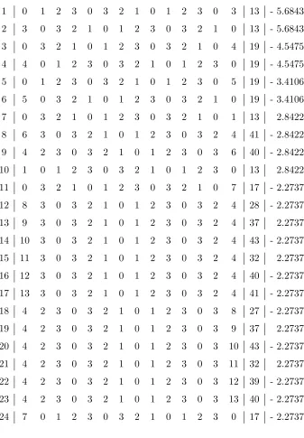
effective key bitsKi, li(K), and finally 107 times the approximation bias. Similarly, linear approximations of 6-round DES with bias in absolute value ≥1.5259×10⁻³ are listed in Table 6.
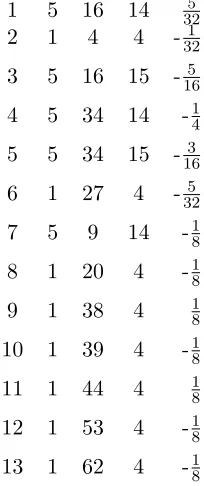
Each row in Table 5 has 5 entries: the 1-round approximation number in the list, the S-box number, input and output masks and the approximation bias.
Table 5: 1-round approximations
1 5 16 14 325 2 1 4 4 -321
3 5 16 15 -165
4 5 34 14 -14
5 5 34 15 -163
6 1 27 4 -325
7 5 9 14 -18
8 1 20 4 -18
9 1 38 4 18
10 1 39 4 -18
11 1 44 4 18
12 1 53 4 -18
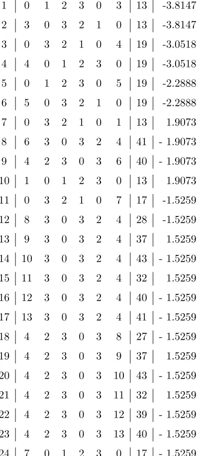
Table 6: Best 6-round approximations
1 0 1 2 3 0 3 13 -3.8147
2 3 0 3 2 1 0 13 -3.8147
3 0 3 2 1 0 4 19 -3.0518
4 4 0 1 2 3 0 19 -3.0518
5 0 1 2 3 0 5 19 -2.2888
6 5 0 3 2 1 0 19 -2.2888
7 0 3 2 1 0 1 13 1.9073
8 6 3 0 3 2 4 41 - 1.9073
9 4 2 3 0 3 6 40 - 1.9073
10 1 0 1 2 3 0 13 1.9073
11 0 3 2 1 0 7 17 -1.5259
12 8 3 0 3 2 4 28 -1.5259
13 9 3 0 3 2 4 37 1.5259
14 10 3 0 3 2 4 43 - 1.5259
15 11 3 0 3 2 4 32 1.5259
16 12 3 0 3 2 4 40 - 1.5259
17 13 3 0 3 2 4 41 - 1.5259
18 4 2 3 0 3 8 27 - 1.5259
19 4 2 3 0 3 9 37 1.5259
20 4 2 3 0 3 10 43 - 1.5259
21 4 2 3 0 3 11 32 1.5259
22 4 2 3 0 3 12 39 - 1.5259
23 4 2 3 0 3 13 40 - 1.5259
Table 7: Best 14-round approximations
1 0 1 2 3 0 3 2 1 0 1 2 3 0 3 13 - 5.6843
2 3 0 3 2 1 0 1 2 3 0 3 2 1 0 13 - 5.6843
3 0 3 2 1 0 1 2 3 0 3 2 1 0 4 19 - 4.5475
4 4 0 1 2 3 0 3 2 1 0 1 2 3 0 19 - 4.5475
5 0 1 2 3 0 3 2 1 0 1 2 3 0 5 19 - 3.4106
6 5 0 3 2 1 0 1 2 3 0 3 2 1 0 19 - 3.4106
7 0 3 2 1 0 1 2 3 0 3 2 1 0 1 13 2.8422
8 6 3 0 3 2 1 0 1 2 3 0 3 2 4 41 - 2.8422
9 4 2 3 0 3 2 1 0 1 2 3 0 3 6 40 - 2.8422
10 1 0 1 2 3 0 3 2 1 0 1 2 3 0 13 2.8422
11 0 3 2 1 0 1 2 3 0 3 2 1 0 7 17 - 2.2737
12 8 3 0 3 2 1 0 1 2 3 0 3 2 4 28 - 2.2737
13 9 3 0 3 2 1 0 1 2 3 0 3 2 4 37 2.2737
14 10 3 0 3 2 1 0 1 2 3 0 3 2 4 43 - 2.2737
15 11 3 0 3 2 1 0 1 2 3 0 3 2 4 32 2.2737
16 12 3 0 3 2 1 0 1 2 3 0 3 2 4 40 - 2.2737
17 13 3 0 3 2 1 0 1 2 3 0 3 2 4 41 - 2.2737
18 4 2 3 0 3 2 1 0 1 2 3 0 3 8 27 - 2.2737
19 4 2 3 0 3 2 1 0 1 2 3 0 3 9 37 2.2737
20 4 2 3 0 3 2 1 0 1 2 3 0 3 10 43 - 2.2737
21 4 2 3 0 3 2 1 0 1 2 3 0 3 11 32 2.2737
22 4 2 3 0 3 2 1 0 1 2 3 0 3 12 39 - 2.2737
23 4 2 3 0 3 2 1 0 1 2 3 0 3 13 40 - 2.2737