Construction of the Database for OMAGE
(Oman Applied General Equilibrium) Model
CoPS Working Paper No. G-288, September 2014
The Centre of Policy Studies (CoPS), incorporating the IMPACT project, is a research centre at Victoria University devoted to quantitative analysis of issues relevant to economic policy. Address: Centre of Policy Studies, Victoria University, PO Box 14428, Melbourne, Victoria, 8001 home page: www.vu.edu.au/CoPS/ email: [email protected] Telephone +61 3 9919 1877
Nhi Tran,
Philip Adams
And
James Giesecke
Centre of Policy Studies,
Victoria University
1
Centre of Policy Studies
Victoria University
Construction of the database for
OMAGE (Oman Applied General Equilibrium) model
September 2014
Nhi Tran1
Philip Adams
James Giesecke
Centre of Policy Studies, Victoria University
Abstract
This paper describes in detail the process to create the database for OMAGE - a Dynamic Applied General Equilibrium model for Oman with labour market detail. It starts with an overview of the model theoretical structure, which consists of a CGE core model and a labour supply module. Then it specifies the coefficients and parameters required for the model database, which provides an initial solution to the model. All data sources and procedures to create the database are then discussed in detail.
2 TABLE OF CONTENTS
1 INTRODUCTION 3
1.1 Overview of OMAGE theoretical structure 3
1.2 Overview of the structure of the OMAGE database 6
1.3 The OMAGE Input – Output database 7
1.4 Sign and balancing conditions for an input-output database 8
1.5 Behavioral parameters 9
1.6 Ancillary data 10
2 THE DATABASE FOR THE CORE OMAGE MODEL 12
2.1 Step 1: Checking the GTAP data for Oman and aggregating it to 46 sectors 13 2.2 Step 2: Disaggregating 46 GTAP sectors into 51 sectors 17
2.3 Step 3: Adjusting sectoral structure 18
2.4 Step 4: Creating margin matrices 18
2.5 Step 5: Creating investment matrices 19
2.6 Step 6: Balancing the database 22
2.7 Step 7: Updating the database to 2012 at the macro level 23
2.8 Step 8: Recreating matrices of indirect taxes 23
2.9 Step 9: Updating the database to 2012 at the sectoral level 24
2.10 Step 10: Compilation of parameters 25
2.11 Step 11: Create wage bill and wage rate matrices 29
2.12 Step 12: Ancilliary data and parameters 29
3 DATA FOR THE LABOUR SUPPLY MODULE 31
3.1 Required data 31
3.2 Data sources 32
3.3 Data compilation procedure 34
4 REFERENCES 45
3
1
INTRODUCTION
This working paper describes the construction of the database for the OMAGE (Oman Applied General Equilibrium) model for the year 2012. In the remainder of this section we first provide an overview of the model theory, before turning to a discussion of the data required by the model. In Section 2 we explain the process by which we turn the format of the supplied data into that required by the model. In Section 3 we present a summary of the input/output data for 2012 in terms of industry cost and sales shares. Data on employment by industry and occupation are also tabled. References are in Section 4.
1.1 Overview of OMAGE theoretical structure
OMAGE has two distinct theoretical parts: (i) the modelling of the economy and its demand for labour by occupation, nationality and skill, hereafter called the core CGE model; and (ii) the modelling of supply of labour by skill, occupation and nationality, hereafter called the labour supply module. Our discussions below focus on these two parts.
1.1.1 Core CGE model
The core CGE structure of OMAGE consists of equations describing: demands for produced inputs and primary factors for current production purposes; commodity supplies by individual industries; industry-specific demands for inputs to capital formation; household commodity demands; export demands distinguished by commodity; government demands distinguished by commodity; the relationship of basic values to production costs and to purchasers' prices; market-clearing conditions for commodities and primary factors; and numerous macroeconomic variables, such as balance of trade, government budget, foreign liabilities and assets.
In OMAGE each industry is assumed to minimise unit costs subject to given input prices and a nested constant returns to scale production function. Three primary factors are identified (labour, capital and land) with labour further distinguished by occupation, nationality and skill. Capital is assumed to be sector-specific, while occupation-specific labour is perfectly mobile across industries. Households are modelled as constrained maximisers of utility functions. Units of new industry-specific capital are cost-minimising combinations of local and foreign commodities. For all commodity users, imperfect substitutability between imported and local varieties of each commodity is assumed. The export demand for any given Omani commodity is inversely related to its foreign-currency price. The model recognises consumption of commodities by government and the details of taxation instruments. It is assumed that all sectors are competitive and all goods markets clear. Purchasers’ prices differ from producer prices by the value of indirect taxes and trade and transport margins. All agents are assumed to be price-takers, with producers operating in competitive markets which prevent the earning of pure profits.
OMAGE is dynamic. The dynamic mechanisms in OMAGE’s core CGE structure include:
4
• accounting for changes in net foreign liabilities via changes in investment and saving; and
• lagged adjustment mechanisms in the labour market.
Capital accumulation is industry-specific, and linked to industry-specific net investment. Annual changes in the net liability position of the economy are related to the annual investment/savings imbalance. In policy simulations, the model provides the option of allowing the labour market to follow a lagged adjustment path. With this option activated, short-run real consumer wages are sticky. Hence short-run labour market pressures mostly manifest as changes in employment. In the long-run, employment returns to baseline, with labour market pressures reflected in changes in real wages.
The theory of the CGE core of OMAGE is based on that of the MONASH model, hence, for details of the full equation system underlying the CGE core of OMAGE, see Dixon and Rimmer (2002).
1.1.2 Labour supply module
The labour supply module contains the mechanism for stock/flow accounting for skill accumulation in the working age population. It starts with the stock of the working age population (WAP) in year 2011 (year t-1 in OMAGE), distinguished by skill, age, gender and citizenship. The WAP in year t is defined as:
(
)
, , ( , ), ,
, , , 1 ( , ), ,
,
a g aa g aa a g a g
s c ss c t ss s c s c
aa AGE ss SKILL
WAP WAP − T NEW
∈ ∈
=
∑
× + (1)where:
, , s c a g
WAP is working age population by age (a), gender (g), citizenship (c), holding skill (s) in year
t;
( 1) , , t ss c aa g
WAP − is working age population of (g,c), having age (aa) and skill (ss) in year t-1;
, , s c a g
NEW is the net number of persons by (a,g,c and s) entering the labour market at the beginning of year t, mainly consisting of people already in Oman turning 15 year of age in t, and net additions of new foreign workers; and
( , ), ( , ), ss s c aa a g
T is a transition matrix showing the rates at which persons (classified by gender and citizenship) move between age categories (movements from age category (aa) to (a)) and skill categories (movements from skill category (ss) to (s)) between years t-1 and t.
The age transition probabilities are calculated based on the number of years in each age group2, and average death rates by age category. The initial qualification transition rates are estimated using educational data on the probability of a group of people by age, gender and citizenship staying within the same qualification or acquiring a different qualification between years t-1 and
t. We expect that the skill dimension of the transition matrix is strongly diagonal, especially for
5 older age groups.
The qualification transition matrix is not static, but has the potential to change from year to year based on changes in relative wage rates between qualifications according to the following equation:
, ,
( , ), ( , ), ( , ), ( , ),
a g c s ss s c ss s c c aa a g aa a g ss
W T AT W α = ×
(2)
where:
( , ), ( , ), ss s c aa a g
AT provides for autonomous shifts in qualification transition rates, allowing for changes in the probability of people changing skill types (qualification fields and/or qualification levels) due to reasons other than changes in the relative wage rates between skills;
ss c
W is the average wage rate for persons holding skill (ss);
, , a g c
α are age-, gender- and citizenship-specific elasticities of qualification transformation with respect to movements in relative wage rates by skill.
Once the stock of working age population by skill is determined, labour supply by skill (LSa gs c,, ) in year t is determined as:
, , , ,
, , , ,
s c s c s c s c a g a g a g a g
LS =WAP ×PR ×ER (3) where
, , s c a g
PR is the labour force participation rate, classified by age, gender, skill and citizenship; and
, , s c a g
ER is the employment rate, classified by age, gender, skill and citizenship. This rate can be determined endogenously under a closure in which wages are determined by another process, or determined exogenously under a closure in which wages are determined endogenously.
The supply of labour distinguished by skill and nationality across occupations is guided by movements in occupation-and-nationality specific wage rates. We assume that workers of nationality c holding skill s allocate labour across occupations so as to maximise a utility function in which the arguments are wage-weighted allocations of labour across occupations and preference variables. The utility maximising solution to this problem, converted to percentage change form, is:3
xo s c, , =xs c, +φo s c, ,
(
wo s c, , −ws c,)
(4)where:
• xo s c, , andwo s c, , are the percentage changes in labour supply and wage rates classified by occupation (o), skill (s) and citizenship (c);
• xs c, and ws c, are percentage changes in labour supply and a measure of average wage
classified by skill and citizenship; and
6
• φo s c, , is the elasticity of labour supply to occupation o by citizen type c with skill s with
respect to movements in the wage available in occupation o relative to other occupations on average.
1.1.3 Linking the core CGE model (Labour demand) and labour supply
OMAGE allows the user to link the core CGE model and the labour supply module via labour markets distinguished by skill, occupation and nationality. On the demand side, industries first chose labour inputs by occupation and nationality based on their demand for primary factors, which, in turn, are based on their level of activity. They then chose a combination of skills to minimise the cost of compiling a unit of labour by occupation and nationality. On the supply side, workers with a given qualification and nationality supply their labour to occupations to maximise a utility function which has hourly wage rates as an argument. Together, labour demand and labour supply in occupation-, qualification- and citizenship-specific labour markets are then reconciled via endogenous movements in wage rates.
The integration of labour demand and labour supply allows endogenous adjustment in the labour market. For example, if a policy change or an economic shock causes a shortage of a particular occupation, the wage of the occupation will rise relative to that of other occupations. This will cause, on the demand side, a relative decline in demand for that occupation from industries compared to other occupations. On the supply side, the rise in the occupation wage rates cause more people to offer to work in the occupation. This, in turn, encourages more people to enroll in qualifications used intensively in that occupation. These adjustments occur until a new equilibrium is established. The integration of labour demand and supply also facilitates the analysis of the economic effects of skill shortages.
However, the model also allows the user to decouple the supply and demand sides, configuring the model as a traditional demand-side forecasting model. This is useful in applications in which we wish to uncover future workforce needs, because it is important that short-run supply-side constraints do not exert an influence on forecast labour needs.
1.2 Overview of the structure of the OMAGE database
The OMAGE model is a system of simultaneous equations, the initial solution to which is provided by the model’s database. The database for OMAGE consists of three main parts:
(1) Input-output (IO) data for the base year;
(2) Behavioural parameters, which govern matters such as how economic agents substitute their input or consumption mix to solve their objective functions when relative prices change; and
(3) Ancillary base year data, relating to industry capital stocks, government accounts, interest rates and the net foreign liability positions of the household and public sectors.
7
1.3 The OMAGE Input – Output database (Figure 1)
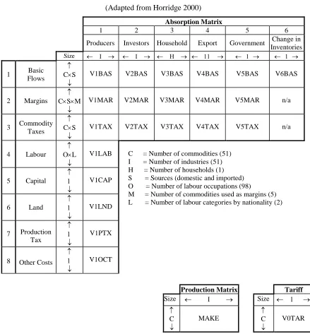
Figure 1 sets out the structure of the OMAGE input-output database in three parts: an absorption matrix, a production matrix, and a tariff matrix.
Figure 1 The OMAGE core input-output database
(Adapted from Horridge 2000)
Absorption Matrix
1 2 3 4 5 6
Producers Investors Household Export Government Change in
Inventories
Size ← Ι → ← Ι → ← Η → ← 11 → ← 1 → ← 1 →
1 Basic
Flows
↑ C×S
↓
V1BAS V2BAS V3BAS V4BAS V5BAS V6BAS
2 Margins
↑ C×S×M
↓
V1MAR V2MAR V3MAR V4MAR V5MAR n/a
3 Commodity
Taxes
↑ C×S
↓
V1TAX V2TAX V3TAX V4TAX V5TAX n/a
4 Labour
↑ O×L
↓
V1LAB C = Number of commodities (51)
I = Number of industries (51) H = Number of households (1) S = Sources (domestic and imported) O = Number of labour occupations (98)
M = Number of commodities used as margins (5) L = Number of labour categories by nationality (2)
5 Capital
↑ 1 ↓
V1CAP
6 Land
↑ 1 ↓
V1LND
7 Production
Tax
↑ 1 ↓
V1PTX
8 Other Costs
↑ 1 ↓
V1OCT
Production Matrix Tariff
Size ← Ι → Size ← 1 →
↑ C ↓ MAKE ↑ C ↓ V0TAR
The column headings in the absorption matrix identify the following users:
(1) Domestic producers divided into I industries; (2) Investors divided into I industries;
(3) A representative household;
8 (6) Changes in inventories.
The first row in the absorption matrix (the “BAS matrices”: V1BAS,…,V6BAS) shows flows in year t of commodities to all users. Each of these matrices has CxS rows, one for each of C commodities from S sources. The flows are valued at basic prices. The basic price of a domestically produced good is the price received by the producer (that is, the price paid by users excluding sales taxes, transport costs and other margin costs). The basic price of an imported good is the landed-duty-paid price, i.e. the price at the port of entry after the commodity has cleared customs.
The second row (the “MAR matrices”: V1MAR,…,V5MAR) shows the values of margin services used to facilitate the flows of commodities identified in the BAS matrices. The commodities used as margins are domestically produced trade, road transport, rail transport, water transport, air transport services, and insurance. Imports are not used as margins services. Each of the margin matrices has CxSxM rows. These correspond to the use of M margin commodities in facilitating flows of C commodities from S sources. We assume that inventories (column 6) comprise mainly of unsold products, and therefore do not bear margins. As with the BAS matrices, all the flows in the MAR matrices are valued at basic prices. Consistent with the UN convention (UN 1999:33), we assume that there are no margins on services.
The third row (the “TAX matrices”: V1TAX,, V5TAX) shows sales taxes on flows to different users. Again, we assume that there are no sales taxes on inventories. The tax rates can differ between users and between sources. For example, tax rates on a commodity used as an intermediate input to producers can be lower than that on household consumption of the same commodity.
Besides intermediate inputs, current production requires inputs of primary factors: labour (divided into occupations and nationality), fixed capital, and land. These are shown in rows 4, 5 and 6. Industries also have to pay production taxes (row 7). Production taxes consist mainly of taxes on the ownership or use of factors of production (UN 1999:26). Examples are fees on licences and permits.
The final two data items in Figure 1 are the MAKE and TARIFF matrices. MAKE is a CxI matrix showing the value of commodity c∈COM produced by industry i∈IND. The TARIFF matrix includes a vector of import duties by import commodity. They are used to calculate the tariff rates in the base year as the ratios between the tariff revenues and the relevant basic flows of imports on which the tariffs are levied.
1.4 Sign and balancing conditions for an input-output database
There are four basic sign and balancing conditions that the database must satisfy.
9 2. Second, the value of output by each industry must equal the total of production costs. That
is, the column sums of the MAKE matrix must equal the sums of the corresponding producers’ columns in the Absorption matrix. This follows from the fact that the current production columns of the Absorption matrix recognise all input costs that form part of production costs at basic prices. This includes the profits earned by owners of the fixed factors employed in each industry.
3. Third, the value of output of domestically produced commodities must equal the total of the value of demands for them. That is, for non-margin commodities, the row sums of the MAKE matrix must equal the sums of the corresponding BAS rows in the Absorption matrix. For margin commodities, their row sums in the MAKE matrix must equal the sum of all direct usage of m (BAS matrix) plus the sum of all usage of m as a margin (MAR matrix). This reflects two features of the database: the valuation basis of the MAKE matrix and absorption matrices are the same, namely, basic prices; and, the columns of the
absorption matrix identify all possible uses of domestically produced goods.
4. Finally, by definition, total value added plus indirect taxes (GDP on the income side) must equal the value of final outputs at market prices (GDP on the expenditure side).
1.5 Behavioral parameters (Figure 2)
Figure 2 lists the various parameters that govern the behaviour of economic agents. In the notation, subscript c indicates commodity (c∈COM) and subscript i indicates industry (i∈IND).
The first three parameters are elasticities which govern the substitutability between factors of production. The first parameter (σprimi(1)) is a vector of elasticities of substitution between labour, capital and land. The second parameter (σlabi(1)) is a vector of elasticities of substitution between different occupations. The parameter σcitizi,o(1)is a matrix of elasticities of substitution between citizens and non-citizens within each occupation and each industry.
The next three parameters σc(1), σc(2)and σc(3)are vectors of Armington elasticities4 which govern commodity-specific domestic/foreign substitution possibilities faced by producers, investors and households respectively.
Parameter εc t, is a vector of foreign demand elasticities for Omani exports by commodity.
Figure 2. ELASTICITIES AND OTHER PARAMETERS
Elasticity of substitution between primary factors (1)
i
prim
σ
Elasticity of substitution between labour occupations (1)
i
lab
σ Elasticity of substitution between domestic and foreign labour (1)
i,o
citiz
σ Elasticity of substitution between domestic and imported intermediate inputs (1)
c σ Elasticity of substitution between domestic and imported inputs to capital formation (2)
c σ
4 Elasticities of substitution between domestic and imported goods, named after Armington (1969 and 1970) who
10
Elasticity of substitution between domestic and imported commodities – household consumption
(3) c σ Export demand elasticities, by commodity
, c t ε Household expenditure elasticities
c
EPS
Frisch parameter F
The last two parameters relate to household consumption: EPScis the vector of household expenditure elasticities; while the Frisch parameter F shows the ratio of households’ total expenditure to their supernumerary expenditure in the Klein-Rubin utility function. The Frisch parameter is used in evaluating household own and cross-price elasticities of demand and in calculating the change in the subsistence component of household consumption.
1.6 Ancillary data (Figure 3 to Figure 6)
1.6.1 Data and parameters for investment and the capital accumulation process
The matrices listed in Figure 3 contain the parameters and data required to operationalise the rate of return and capital accumulation theory in the model. They include capital stocks Ki, depreciation rates Di, and historical normal capital growth rates Kgrtrend i, . Other parameters and
data include the difference between trend capital growth rates and maximum capital growth rates (coefficient DIFF); the reciprocal of the slope of the economy-wide capital supply function
i
C in the vicinity of Kgri= Kgrtrend i, , the real interest rate (R) and the inflation rate. The inflation rate is calculated from the levels of the national CPI in years t and t-1 (CPIt−1 and CPIt).
Figure 3. INVESTMENT AND CAPITAL Value of capital in the base year
i
K
Depreciation rates
i
D
Trend growth rates of capital
, trend i
Kgr
Difference between max. and trend growth rates of capital DIFF Average sensitivity of capital growth to variations in expected rates of return
i
C
Level of the CPI – lagged
1 t
CPI−
Level of the CPI
t
CPI
Real interest rate R
1.6.2 Data and parameters for the labour market
11 national aggregate employment indexEt, and the value of the parameter α1, which governs the speed with which aggregate employment in the policy deviation run returns to its forecast value.
Figure 4LABOUR MARKET
Wages in the base year by industry, occupation, and nationality
, , i occ citizenship
W
Index of CPI deflated wages
b
W
Index of aggregate employment
t
E
Parameter governing duration of non-zero employment deviations
1
α
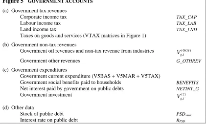
1.6.3 Government accounts
Figure 5 lists the data needed for the government accounts. They include aggregate items for government revenues and expenditures, as well as the government debt. Revenues include tax and non-tax sources. The direct taxes include taxes on labour, capital and land incomes (TAX_LAB,TAX_CAP and TAX_LND). These taxes are used for calculating tax rates on factors of production, by dividing tax revenues by the relevant factor income base. Note that indirect taxes are already included in Figure 1. Government non-tax revenues include government oil revenues, and government services and investment revenues. Government expenditure include government current expenditure, government social welfare paid to households (BENEFITS), net interest paid by government on public debt (NETINT_G), and government investment by industry (Vg i(2), ). The net interest paid by government on public debt is calculated using the value of government debt stock at the start of the base year (PSDstart) and the rate of interest on public debt (RPSD). With these data, the model can trace the government account balance during
simulations.
Figure 5 GOVERNMENT ACCOUNTS
(a) Government tax revenues
Corporate income tax TAX_CAP
Labour income tax TAX_LAB
Land income tax TAX_LND
Taxes on goods and services (VTAX matrices in Figure 1)
(b) Government non-tax revenues
Government oil revenues and non-tax revenue from industries ( ) , GOS g i
V
Government other revenues G_OTHREV
(c) Government expenditures
Government current expenditure (V5BAS + V5MAR + V5TAX)
Government social benefits paid to households BENEFITS
Net interest paid by government on public debts NETINT_G
Government investment (2)
, g i
V
(d) Other data
Stock of public debt PSDstart
12
1.6.4 Accounts with the rest of the world
Figure 6 lists additional data needed to calculate accounts with the rest of the world. They include stocks of net foreign liabilities in the base year (FDATT), rates of interest on those liabilities (ROIFOREIGN), and grants and remittances from Rest of World to Oman (GRANTS, FPTRANS).
Figure 6 ACCOUNTS WITH THE REST OF THE WORLD
Net foreign liabilities in the base year FDATT
Rate of interest on net foreign liabilities ROIFOREIGN
Grants from foreigners GRANTS
Remittances from Rest of Word FPTRANS
2
THE DATABASE FOR THE CORE OMAGE MODEL
Our aim is to build a model which represents the Oman economy in 2012, the latest year for which key economic data required for the model are publicly available at the time of this database construction.
Sources for the data items discussed in the previous section include:
• Oman input-output data for the year 2007 and elasticities in the GTAP 8.0 database (Narayanan et al. 2012). This database is a global database describing bilateral trade patterns, production, consumption and intermediate use of commodities and services for just under 130 countries/regions in the World. More discussion about this Oman database can be found in Section 2.1.
• Oman Statistical yearbooks for the years 2010-2013 (NCSI 2011, 2012, 2013a, 2013b), which contain statistics on national accounts and sectoral variables, such as gross output, gross value added and payment to labour for the period 1998 - 2012. These data are used to (i) split the GTAP database into more relevant sectors for Oman (e.g. one sector in GTAP includes public administration, education and healthcare. We wanted to model each of these activities separately); and (ii) to update the database from 2007 to 2012. The Yearbooks also contains data on government and foreign accounts required for data items in Figures 5 and 6 above. More discussions on these procedures are included in Section 2.2.
• Oman Census 2010 data (NCSI 2013c), which contain data on the number of employed persons by industry, occupation, age, gender, nationality (Omani/NonOmani),
qualification level and qualification fields. This data is used to compile the employment matrix by industry, occupation and nationality.
13 occupation and nationality. These wage rates are used together with the number of workers from Census to compile the wage bill matrix V1LAB in Figure 1.
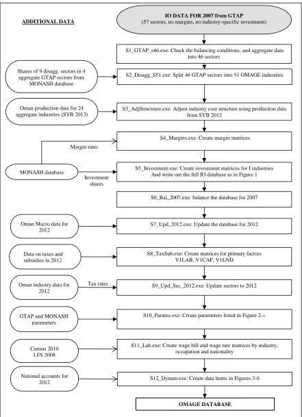
The input-output database for OMAGE was compiled in 12 steps as illustrated in Figure 7 below. To promote transparency and assist trouble shooting, we automated the process of generating the OMAGE database by using GEMPACK (Harrison and Pearson 1996).5 Much of our initial input data was provided to us in Excel format. We converted this to GEMPACK’s Header Array format using ViewHAR (Horridge 2014). For each step of the database creation process, we wrote a TABLO program to conduct the necessary calculations and manipulations. They are listed in rectangular boxes in Figure 7. An important part of each TABLO program at each step is a series of checks to ensure that the data meet necessary balance and other conditions at each stage of the data creation process (see Section 1.4). Batch files automate the execution of the series of TABLO-generated programs. We think our approach has a number of advantages, particularly relative to the common alternative of doing large numbers of sequential data manipulations using a spreadsheet program like Excel. First, it is transparent. TABLO input files are text files written in an easy to master language. As such, each TABLO program represents transparent documentation of the data manipulation processes that we have implemented at each stage of the database creation process. Second, automation enables timely generation of an updated database, as required.
2.1 Step 1: Checking the GTAP data for Oman and aggregating it to 46 sectors
Our starting point for the database is Oman data in the GTAP database for the year 2007, denominated in million US dollars. In this first step we first checked the GTAP data to see whether they satisfy the balancing and sign conditions, and then checked whether the GTAP data set contains all the matrices required for the OMAGE model as specified in Figure 1. We found that the GTAP data satisfy the sign and the balancing conditions. However, the data set itself does not distinguish all the detail required. In particular:
1. It does not distinguish trade and transport margins on commodity flows from producers to users of commodities. That is, it does not have the matrices V1MAR – V5MAR listed in Figure 1. Distinguishing margins is important for properly accounting for the contributors to market prices, and hence better assessment of impacts of policy changes. We, therefore, will need to create these margin matrices.
5 GEMPACK was created at, and is maintained by, the Centre of Policy Studies. It is designed specifically for CGE
14
Figure 7. Steps in creating the database for the core OMAGE model, data sources, and
execution programs
Margin rates
S12_Dynam.exe: Create data items in Figures 3-6 S8_TaxSub.exe: Create matrices for primary factors
V1LAB, V1CAP, V1LND
IO DATA FOR 2007 from GTAP
(57 sectors, no margins, no industry-specific investment)
ADDITIONAL DATA
S1_GTAP_s46.exe: Check the balancing conditions, and aggregate data into 46 sectors
S2_Disagg_S51.exe: Split 46 GTAP sectors into 51 OMAGE industries
Tax rates
S4_Margins.exe: Create margin matrices
Investment shares
S10_Params.exe: Create parameters listed in Figure 2-+ GTAP and MONASH
parameters
Census 2010 LFS 2008
S3_AdjStructrure.exe: Adjust industry cost structure using production data from SYB 2013
Data on taxes and subsidies in 2012
S6_Bal_2007.exe: balance the database for 2007
S9_Upd_Sec_2012.exe: Update sectors to 2012 Oman industry data for
2012
S7_Upd_2012.exe: Update the database for 2012 Oman Macro data for
2012
S5_Investment.exe: Create investment matrices for I industries And write out the full IO database as in Figure 1 MONASH database
S11_Lab.exe: Create wage bill and wage rate matrices by industry, occupation and nationality
OMAGE DATABASE
Shares of 9 disagg. sectors in 4 aggregate GTAP sectors from
MONASH database
Oman production data for 24 aggregate industries (SYB 2013)
15 2. It does not distinguish investment by industry. That is, it does not have the matrices
V2BAS, V2MAR and V2TAX as listed in Figure 1. There is only one investment column showing the use of commodities for investment purposes. In addition, the column seems to contain goods used for investment (i.e. fixed capital formation) and goods going into inventories. For example, the investment column contains non-zero values for pure consumer goods such as meat, dairy, rice, beverages and tobacco products. We will need to split the “Investment” column into the 51 columns representing the investment activity of each of the industries in OMAGE.
Importantly, the sectoral disaggregation of the GTAP database is not entirely suitable for the Omani economy. For example, out of its 57 sectors, GTAP data distinguish 14 agricultural, forestry and fishery industries, which are of relatively little importance to Oman. On the other hand, GTAP data have a higher level of aggregation for services sectors than what is desirable for Oman. For example, public administration, education and health are represented by only one sector, whereas it is desirable that these sectors are treated separately. Hence, as can be seen from Table 1 below, we created for OMAGE a database with 51 sectors, where there are fewer agricultural and food processing sectors but more services sectors than that in GTAP.
In the first step (Step 1), we aggregated the more detailed agricultural, mining and food processing sectors in GTAP into the level of aggregation adopted in the final OMAGE database (see the first half of Table 1). After this step, the database contained 46 sectors. In the next step (Step 2), some services sectors are disaggregated (see the second half of Table 1).
At this point we converted the database from USD million into Omani Rials million, using the exchange rate of 0.386 OMR/USD. This exchange rate was calculated as the ratio of the GDP for Oman in 2007 measured in OMR to that measured in USD as published in the World Development Indicators database (World Bank 2013).
Table 1. Concordance between sectors in GTAP data, Omani production account data,
and the adopted sectors for the OMAGE database
A. GTAP sectors B. Sectors with data from NCSI C. Adopted sectors 1. Paddy rice
1.Agriculture 1.Cereals 2.Wheat
3.Cereal grains n.e.c.6
4.Vegetable, fruits, nuts 2.Fruits and vegetables
5.Oil seeds
3.Other crops 6.Sugar cane, sugar beet
7.Plant-based fibers
8.Crops n.e.c.
9.Forestry
10.Bovine cattle, sheep and goats, horses
4.Live stock
16
A. GTAP sectors B. Sectors with data from NCSI C. Adopted sectors 11.Animal products n.e.c.
12.Raw milk
13.Wool, silk-worm cocoons
14.Fishing 2.Fishing 5.Fishing
15.Coal 3.Mining of non-ferrous metal ores 6.Coal
16.Oil
17.Gas extraction
4.Extraction of crude petroleum 7.Oil
8.GasExtract 5.Extraction of natural gas
6.Services incidental to oil and gas7
18.Minerals n.e.c. 7.Other mining and quarrying 9.Minerals n.e.c.
19.Bovine meat. 8.Other manufacturing 10.Meat products
20.Meat product n.e.c 11.Meat products
21.Vegetable oils and fats 12.Vegetable oils and fats
22.Dairy products 13.Dairy products
23.Processed rice 14.Processed rice
24.Sugar 15.Sugar
25.Food products n.e.c. 16.Food products n.e.c.
26.Beverages and tobacco products 17.Beverages and tobacco products
27.Textiles 18.Textiles
28.Wearing apparel 19.Wearing apparel
29.Leather products 20.Leather products
30.Wood products 21.Wood products
31.Paper products, publishing 22.Paper products, publishing
32.Petroleum, coal products 9.Manufacturing of refined petroleum products
23.Petroleum, coal products
33.Chemical, rubber, plastic products 10.Manufacturing of chemicals 24.Chemical, rubber, plastic products
34.Mineral products n.e.c. 25.Mineral products n.e.c.
35.Ferrous metals 26.Ferrous metals
36.Metals n.e.c. 27.NonFeMetals
37.Metal products 28.Metal products
38.Motor vehicles and parts 29.Motor vehicles and parts
39.Transport equipment n.e.c. 30.Transport equipment n.e.c.
40.Electronic equipment 31.Electronic equipment
41.Machinery and equipment n.e.c. 32.Machinery and equipment n.e.c.
42.Manufactures n.e.c. 33.Manufactures n.e.c.
43.Electricity
11.Electricity and water supply
34.Electricity
44.Gas 35.Gas
45.Water 36.Water
7 Although the SYB provides data on output and value added for this "Services incidental to oil and gas" sector,
17
A. GTAP sectors B. Sectors with data from NCSI C. Adopted sectors 46.Construction 12.Building and construction 37.Construction
47.Trade 13.Wholesale and retail trade 38.Wholesale and retail trade
14.Hotels and restaurants 39.Hotels and restaurants
48.Transport n.e.c. 15.Land transport 40.Land transport
16.Supporting and auxiliary transport activities
41.Transport n.e.c.
49.Water transport 42.Water transport
50.Air transport 17.Air transport 43.Air transport
51.Communication 18.Post and telecommunication 44.Communication
52.Financial services n.e.c. 19.Financial intermediation, except insurance
45.Financial services n.e.c.
53.Insurance 20.Insurance and pension trust 46.Insurance
54.Business services n.e.c. 21.Real Estate 47.Real Estate
22.Business activities 48.Business services n.e.c. 55.Recreational and other services 23.Other community, social and
personal services
49.Recreational and other services
24.Private household with employed persons
56.Public Administration, Defense, Education, Health
25.Public administration and defence 50.Public administration and defence
26.Education 51.Education
27.Health 52.Health
57.Dwellings 53.Dwellings
2.2 Step 2: Disaggregating 46 GTAP sectors into 51 sectors
In this step we conducted the following disaggregations:
1. The Trade, Hotel and Restaurant sector was disaggregated into two separate industries – Trade, and Hotels and restaurants;
2. The Other Transport sector was disaggregated into two industries - Land transport, and Transport services;
3. The Other Business services sector was disaggregated into two industries - Real estate, and Other business services; and
4. The Government, Education and Health sector was disaggregated into three industries - Public administration, Education, and Health.
The disaggregation required us to know the cost and sale structures of the new sectors. We borrowed these structures from the MONASH database for the Australian economy. We then used the RAS procedure to scale the data so that the newly created sectors summed to their original sectors.8 After this step, the database contained 51 sectors as described in Column (c), Table 1 above.
8 RAS is a method in which a bi-proportional technique is used to scale a matrix to specified targets, often the row
18
2.3 Step 3: Adjusting sectoral structure
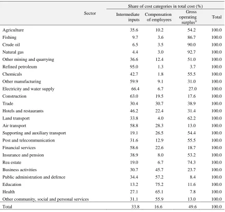
Statistical Yearbook 2013 (NCSI 2013b) provides data for output and broad production cost categories for 27 sectors in the economy for the period 2007 -2012. We aggregated the 27 sectors to 24 sectors to which OMAGE 51 sectors can map, and then calculated the average shares of different cost categories for the period to get a representative cost structure for the sectors, as reported in Table 2. We then adjusted the GTAP database to reflect these structures.
Table 2. Cost structure for 24 aggregate sectors
Sector
Share of cost categories in total cost (%)
Intermediate inputs
Compensation of employees
Gross operating surplus9
Total
Agriculture 35.6 10.2 54.2 100.0
Fishing 9.7 3.6 86.7 100.0 Crude oil 6.5 3.5 90.0 100.0
Natural gas 4.4 3.0 92.7 100.0 Other mining and quarrying 36.6 12.4 51.0 100.0
Refined petroleum 95.0 1.3 3.7 100.0
Chemicals 42.7 1.8 55.5 100.0 Other manufacturing 59.9 9.1 31.0 100.0
Electricity and water supply 66.4 6.7 27.0 100.0 Construction 63.0 19.5 17.6 100.0
Trade 30.4 30.7 38.9 100.0
Hotels and restaurants 46.2 22.4 31.4 100.0 Land transport 33.8 4.0 62.2 100.0
Air transport 58.8 28.3 13.0 100.0 Supporting and auxiliary transport 19.1 26.5 54.4 100.0
Post and telecommunication 31.6 12.9 55.5 100.0
Financial services 58.6 22.6 18.7 100.0 Insurance and pension 38.9 8.0 53.2 100.0
Rea estate 19.0 6.7 74.3 100.0 Business activities 30.7 45.7 23.7 100.0
Public administration and defence 34.4 57.2 8.4 100.0
Education 13.2 75.2 11.6 100.0 Health 27.1 65.1 7.8 100.0
Other community, social and personal services 31.1 55.9 13.0 100.0
Total 33.8 16.6 49.6 100.0
(Source: Calculated for the period 2007-2012 from NCSI 2013a, “Production account by kind of economic activity at current prices”)
2.4 Step 4: Creating margin matrices
In this step we created the margin matrices. This involved two steps. First, we distinguished between direct and margin usage of a margin commodity. Then we allocated the margin usage
19 to different commodity flows to different users.
Margin commodities (such as road transport) can be used either directly, or as a margin service. Margin services facilitate the flows of goods from producer to user, while direct purchases are valued in their own right. For example, consider road transport services. Purchase of a taxi ride by a banker to get from one office to another is a direct intermediate input of road transport services to thebanking industry. Purchase of truck delivery service to deliver furniture from a shop to a bank office is a purchase of a road transport margin service by the banking industry.
The GTAP database contains five margin commodities (namely Trade, Land transport, Water transport, Air transport, and Supporting and auxiliary transport). However, it does not distinguish direct and margin uses of these commodities. It also does not contain information on the margin rates on each commodity flow. We borrowed this information from the MONASH database. First, we calculated the direct use of margin commodities by assuming that, for each margin commodity, the share of direct use in total use of the commodity by each user is the same as that in the MONASH database. For example, the direct use of margin commodities by households is 20% for trade, 41% for land transport, 96% for water transport, 97% for air transport, and 92% for supporting and auxiliary transport services. For each margin commodity, the margin use is the difference between total use and direct use. We then calculated the margin matrices with the assumption that for each commodity, all the margin rates are the same on intermediate inputs and investment for all producers, and the margin rates are also the same for commodities used by other final consumption categories. We calculated these rates from the MONASH database. Then we multiplied the rates with the USE matrix to get the initial margin values. The initial margin values were then scaled so that they sum up to the margin use of each margin commodity.
2.5 Step 5: Creating investment matrices
The OMAGE model requires each industry to be an investor. The investor buys commodities to construct capital units specific to their industry. However, in the original GTAP database there is only a single investor for the whole economy, represented in a single column. In this step, we split that column into 51 columns, as required in Column 2, Figure 1.
This task involved two main stages. In the first stage, we calculated the amount of total investment undertaken by each industry in the base year. The sum of investment across industries must equal the GDP (expenditure side) estimate of economy-wide investment. In the second stage, we calculated the commodity-composition of each industry’s investment. The total use of each commodity for investment purposes across all industries must be the same as the value of that commodity in the single investment column in IO table. In the section below we describe the procedure in more detail.
2.5.1 Stage 1: Estimating industry investment and capital stock
20 1. Aggregate gross fixed capital formation, valued at RO 4,638.6 million.
2. Investment by 16 aggregate sectors, as reported in Table 3 below.
Table 3. Sectoral investment in 2007 (RO mil)
Sector Value Corresponding OMAGE industries10
Agriculture and fisheries 12.2 Cereals, VegFruits, OthCrops, Livestock, Fishing
Crude oil 1,210.6 CrudeOil Natural gas 381.9 NatGas
Other mining and quarrying 9.9 OthMining
Manufacturing 1,060.3 Meat, OilFats, Dairy, Rice, Sugar, OthFood, BevTobacco,
Textile, Clothing, LeatherProd, WoodProd, PaperPublish, PetrolCoke,
ChemRubPlast, NMetalProd, FeMetal, NFeMetals, MetalProds, MotorVehicle,
OthTransEq, ElectronicEq, OthMachEq, OthManuf Electricity and water supply 163.4 Electricity, Gas, Water
Construction 172.5 Construction Wholesale and retail trade 97.0 Trade
Hotels and restaurants 53.4 HotelsRest
Transport, storage and communication 254.8 LandTrans, WaterTrans, AirTrans, OthTrans, Communicatn
Financial intermediation 56.9 FinanceServ, Insurance
Real estate, renting and business activities 367.8 RealEstate, OthBusServ
Public administration and defence 513.8 PublicAdmin Education 99.8 Education
Health 25.0 Health Other community, social and personal services 159.1 RecrOthServ
Total 4638.6
(Source: NCSI 2013a, Table 17-14, adjusted to meet the value of aggregate Gross Fixed Capital Formation in
National Account).
We first allocated the value of investment by 16 aggregate sectors to more disaggregated industries within each sector (see column 3, Table 3) in proportion to industry shares in capital rentals of the aggregated sector. We then checked to see if these initial estimates are plausible by calculating industry rates of return based on the following equation: for each industry,
𝑅𝑅=𝐺𝐺𝐺𝐺𝐺𝐺(𝑘𝑘𝐼𝐼+𝐷𝐷)− 𝐷𝐷 (5)
where R is the net rate of return on an industry’s capital stock (e.g. a number like 0.05), I is industry investment, GOS is gross operating surplus, k is the industry’s capital growth rate, defined as 𝑘𝑘 =𝐾𝐾1
𝐾𝐾0−1 (e.g. a number like 0.01), and D is the industry’s depreciation rate (e.g.
a number like 0.07). Equation (5) is derived from the following equations:
10 Due to space limit, industries are listed with their short names here. See Appendix 1 of this document to see their
21 1) The capital accumulation formula:
1 0(1 )
K =K −D +I (6)
where andK1 are the industry’s capital stock at the beginning and the end of the year; D is the industry’s depreciation rate; and I is the value of investment in the industry during the year; and
2) The equation for calculating net rate of return on industry capital stock:
1 0
GOS
R D
K
= − (7)
where R1 is the net rate of return on the industry’s capital in the period, defined as the ratio of capital rental in the industry (GOS) to the value of its capital stock (K0), less depreciation rate
(D).
To implement (5), we already have GOS from the database. We adopted industry depreciation rate D from BEA (2013) estimates for American industries for the year 2012. The rates range from 0.033 for real estate to 0.17 for the manufacturing of electronic equipment. The economy-wide average depreciation rate is 0.082. As for industry capital growth rates (k), we assumed that capital stock grew at the same rates as industry real value added over the period 2007-2012. We calculated these real growth rates of value added from national accounts data (NCSI 2013a). On average, the growth rate is 0.052 (or 5.2%). With the initial estimates for I discussed earlier, we calculated the initial values of R based on equation (5). These initial values for R vary substantially between industries, from 0.39 for agriculture to negative 0.11 for public administration and defence. We do not believe this wide dispersion of R, and hence we adjusted R according to the following formula:
𝑅𝑅1 =𝑅𝑅𝑎𝑎𝑎𝑎𝑎𝑎𝛼𝛼 𝑅𝑅01−𝛼𝛼 (8)
where R0 and R1 are industry initial and adjusted rates of return respectively; α is the weight
with which we weigh industry rate of return and economy-wide average rate of return Rave. We
adopted the value of 0.8 for α, and the value of 0.0286 for economy-wide average rate of return on capital. The latter value (2.86 %) is the average lending rate over the period 2003-2012 in Oman (World Bank 2013).
After calculating R1, we recalculated industry investment value (I) using equation (5), and then scaled them so as they sum to economy-wide aggregate capital formation values as reported in the national accounts. We then calculated industry capital stocks using the following formula that is derived from equation (6) above:
𝐾𝐾=𝑘𝑘+𝐼𝐼 𝐷𝐷 (9)
0
22
2.5.2 Stage 2: Calculating the composition of investment
After estimating the value of investment by industry, we estimated the commodity input requirements for each industry’s investment. Industry-specific capital input requirements are mainly governed by the nature of the industry. For example, we would expect investment in transport service sectors to be comprised mainly of transport equipment. Similarly, we might expect units of new capital in agricultural sectors to have a high requirement for inputs of agricultural machinery. We formed an initial guess at industry-specific input requirements to capital formation using shares from Australian data. These shares can be replaced in the data creation algorithm at a later date if specific information on the composition of investment by industry in Oman becomes available.
We first multiplied the total value of investment in each industry (calculated in Stage 1) by our initial estimate of shares of source-specific commodity inputs to each industry’s capital formation. This produced an initial estimate of the basic value of each source-specific commodity flow to the capital creation activity of each industry. We then applied tax and margin rates from the IO table output from the previous step to produce the tax and margin flows on these commodities. Finally, we applied the RAS procedure to the investment matrices so that (i) the commodity, tax and margin row sum to their values in the investment columns for basic, tax and margins in the previous step; and (ii) the columns sums to the value of industry investment.
2.6 Step 6: Balancing the database
In this step we balanced the database and target some macro variables using the Adjuster program developed by Horridge (2009). This program provides a better approach than simple RAS or similar iterative methods, in which each scale factor is adjusted to meet one constraint only. In the Adjuster program, all coefficients in the IO database and macroeconomic variables are simultaneously connected via equations describing the balancing conditions in the database and the macroeconomic relationships in the model. The equations include scaling variables which allow the coefficients to adjust so as to meet exogenously determined targets. The targets may include balancing constraints, such as the zero-pure profit conditions, or the values of GDP and its components as available from the national accounts.
23
Table 4. GDP components in 2007 and 2012, RO mil
GDP components 2007 2012
Household consumption 4,955.5 8,782.1
Government consumption 3,043.9 5,718.1
Gross capital formation 5,513.70 7,336.60
Exports 9,139.8 18,667.0
Imports 6,471.0 10,706.0
GDP 16,181.8 29,797.7
(Source: NCSI 2013b, Section 14 – National Accounts)
2.7 Step 7: Updating the database to 2012 at the macro level
We used the Adjuster program (Horridge 2009) to update the database from 2007 to 2012, using the values of macro variables as reported in column 2, Table 4. This scaled the whole database proportionately so as to achieve these values. However, during the period 2007-2012 different sectors may have developed differently. These differences in sectoral development are taken into account in Step 9. In Step 8 below, we recalculate taxes and subsidies in the database.
2.8 Step 8: Recreating matrices of indirect taxes
There are two main types of indirect tax in OMAGE: taxes and subsidies on products (hereafter commodity taxes) and other taxes and subsidies on production (hereafter production taxes). In the original and updated GTAP data, total net (taxes less subsidies) indirect tax revenues are positive. However, the Omani national accounts show that the total net indirect tax revenues become negative in 2012. One of the causes of this is the addition of subsidies on oil product in 2012, which did not exist in 2007 (see Table 2-15 in Chapter 15 “Public Finance” in NCSI (2011, 2013b)). Therefore, there is a need to recalculate the net indirect tax matrices V1TAX - V5TAX and PTAX in the model. Table 5 reports the values and our assumptions about the incidence of the taxes/subsidies that were used to create the net tax matrices in OMAGE.
Table 5. Indirect taxes and subsidies in 2012 (RO mil)
Items Value Assumed tax incidence for tax allocation
(a) Taxes 349.6
Business and professional Licences 9.2 Production tax on all industries, except Agriculture,
Public administration, and Dwellings services
Vehicle licences 39.3 Tax on the use of Motor vehicles by all users
Hotels & entertainments taxes 19.1 Tax on the use of Hotels, restaurants and Recreation
services by all users Taxes on concessionary use of airports &
seaports
18.5 Tax on the use of Water transport and Air transport by all users
Taxes on building permits 1.6 Production tax on the Construction industry
Miscellaneous taxes 11.8 Tax on all commodities from both sources, by all users
Communication services-licensing fees 0.0 Production tax on the Communication industry
Customs duties 250.1 Tariff on all imported products
(b) Subsidies 1,260.3
24
Oil products 1,007.7 Subsidy on the use of refined petroleum by all users
Net indirect taxes -910.7
(Source: NCSI 2013a, Section 15 – Public Finance)11
For each of the taxes/subsidies in Table 5, except for Custom duties, we allocated the tax/subsidy revenue proportionately to the values of commodity flows or production listed in the Incidence column. For Custom duties, we scaled the existing tariff revenues in the database to the value reported in Table 5.
2.9 Step 9: Updating the database to 2012 at the sectoral level
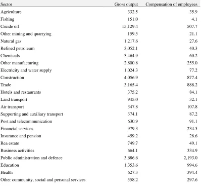
In this step we used the Adjuster program (Horridge 2009) to update not only macro, but also selected sectoral variables for the year 2012. Specifically, we targeted the gross outputs and compensation of employees for selected sectors in the 24 aggregate sectors as published in NCSI (2013a), and reported in Table 6.
Table 6. Sectoral gross output and Compensation of employees in 2012 (RO mil)
Sector Gross output Compensation of employees
Agriculture 332.5 35.9
Fishing 151.0 4.1
Cruide oil 15,129.4 507.7
Other mining and quarrying 159.5 21.1
Natural gas 1,217.6 27.6
Refined petroleum 3,052.1 40.3
Chemicals 3,464.9 60.2
Other manufacturing 2,800.8 255.0 Electricity and water supply 1,024.3 77.2
Construction 4,056.9 877.4
Trade 3,165.4 888.2
Hotels and restaurants 375.2 84.1
Land transport 945.0 32.1
Air transport 347.8 107.8
Supporting and auxiliary transport 374.1 87.2
Post and telecommunication 630.9 91.1 Financial services 979.3 234.5
Insurance and pension 459.2 28.6
Rea estate 749.7 49.1
Business activities 664.1 334.9
Public administration and defence 3,686.6 2,193.0
Education 1,353.6 994.6
Health 627.3 394.4
Other community, social and personal services 558.2 297.6
11 Note that the net indirect tax revenues calculated in this Table is slightly higher than the value of -1,001.4 reported
25
Sector Gross output Compensation of employees
Total 46,305.4 7,723.7
(Source: NCSI 2013a, Production account by kind of economic activity at current prices)
We also targeted export values of important products, such as oil, chemicals, foods and beverages, and other goods and services for which data are available for 2012.
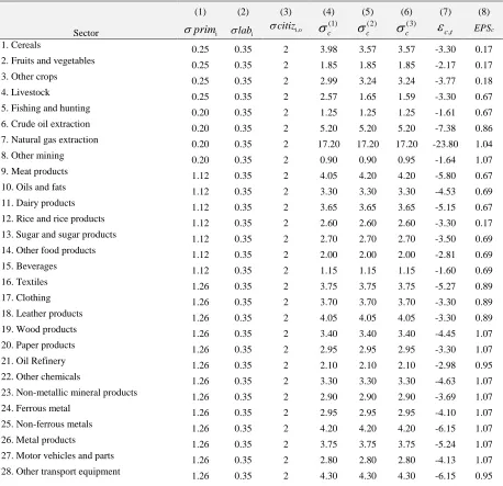
2.10 Step 10: Compilation of parameters
In this step we compiled the parameters described in Figures 2. As there are no parameter estimates for Oman, we adopted them from the GTAP database and/or from the MONASH model. The values of the industry or commodity parameters are reported in Table 7. We discuss them below.
Table 7. Industry/commodity parameters for OMAGE
(1) (2) (3) (4) (5) (6) (7) (8)
Sector σprimi σlabi i,o
citiz
σ (1)
c
σ (2)
c
σ (3)
c
σ εc t, EPSc 1. Cereals 0.25 0.35 2 3.98 3.57 3.57 -3.30 0.17
2. Fruits and vegetables 0.25 0.35 2 1.85 1.85 1.85 -2.17 0.17
3. Other crops 0.25 0.35 2 2.99 3.24 3.24 -3.77 0.18 4. Livestock 0.25 0.35 2 2.57 1.65 1.59 -3.30 0.67
5. Fishing and hunting 0.20 0.35 2 1.25 1.25 1.25 -1.61 0.67 6. Crude oil extraction 0.20 0.35 2 5.20 5.20 5.20 -7.38 0.86
7. Natural gas extraction 0.20 0.35 2 17.20 17.20 17.20 -23.80 1.04
8. Other mining 0.20 0.35 2 0.90 0.90 0.95 -1.64 1.07 9. Meat products 1.12 0.35 2 4.05 4.20 4.20 -5.80 0.67
10. Oils and fats 1.12 0.35 2 3.30 3.30 3.30 -4.53 0.69 11. Dairy products 1.12 0.35 2 3.65 3.65 3.65 -5.15 0.67
12. Rice and rice products 1.12 0.35 2 2.60 2.60 2.60 -3.30 0.17
13. Sugar and sugar products 1.12 0.35 2 2.70 2.70 2.70 -3.50 0.69 14. Other food products 1.12 0.35 2 2.00 2.00 2.00 -2.81 0.69
15. Beverages 1.12 0.35 2 1.15 1.15 1.15 -1.60 0.69 16. Textiles 1.26 0.35 2 3.75 3.75 3.75 -5.27 0.89
17. Clothing 1.26 0.35 2 3.70 3.70 3.70 -3.30 0.89
18. Leather products 1.26 0.35 2 4.05 4.05 4.05 -3.30 0.89 19. Wood products 1.26 0.35 2 3.40 3.40 3.40 -4.45 1.07
20. Paper products 1.26 0.35 2 2.95 2.95 2.95 -3.30 1.07 21. Oil Refinery 1.26 0.35 2 2.10 2.10 2.10 -2.98 0.95
22. Other chemicals 1.26 0.35 2 3.30 3.30 3.30 -4.63 1.07
23. Non-metallic mineral products 1.26 0.35 2 2.90 2.90 2.90 -3.69 1.07 24. Ferrous metal 1.26 0.35 2 2.95 2.95 2.95 -4.10 1.07
25. Non-ferrous metals 1.26 0.35 2 4.20 4.20 4.20 -6.15 1.07 26. Metal products 1.26 0.35 2 3.75 3.75 3.75 -5.24 1.07
27. Motor vehicles and parts 1.26 0.35 2 2.80 2.80 2.80 -4.13 1.07
26
(1) (2) (3) (4) (5) (6) (7) (8)
Sector σprimi σlabi i,o
citiz
σ (1)
c
σ (2)
c
σ (3)
c
σ εc t, EPSc 29. Electronic equipment
1.26 0.35 2 4.40 4.40 4.40 -6.50 1.07 30. Other machinery and equipment 1.26 0.35 2 4.05 4.05 4.05 -5.88 1.07
31. Other manufacturing 1.26 0.35 2 3.75 3.75 3.75 -5.51 1.07 32. Electricity 1.26 0.35 2 2.80 2.80 2.80 -3.30 1.04
33. Gas distribution 1.26 0.35 2 2.80 2.80 2.80 -4.19 1.04 34. Water, sewerage and drainage
1.26 0.35 2 2.80 2.80 2.80 -3.30 1.04 35. Construction services 1.40 0.35 2 1.90 1.90 1.90 -3.30 1.04
36. Wholesale and retail trade services 1.68 0.35 2 1.90 1.90 1.90 -3.30 1.11 37. Accommodation and restaurants 1.68 0.35 2 1.90 1.90 1.90 -2.85 1.11
38. Land transport services 1.68 0.35 2 1.90 1.90 1.90 -2.85 0.95 39. Water transport services
1.68 0.35 2 1.90 1.90 1.90 -2.85 0.95 40. Air transport services 1.68 0.35 2 1.90 1.90 1.90 -2.85 0.95
41. Other transport services 1.68 0.35 2 1.90 1.90 1.90 -2.85 0.95 42. Communications 1.26 0.35 2 1.90 1.90 1.90 -2.85 0.95
43. Financial services 1.26 0.35 2 1.90 1.90 1.90 -2.85 1.25 44. Insurance services
1.26 0.35 2 1.90 1.90 1.90 -2.85 1.04 45. Real estate services 1.26 0.35 2 1.90 1.90 1.90 -3.30 1.25
46. Other business services 1.26 0.35 2 1.90 1.90 1.90 -2.85 1.25 47. Public administration and defence 1.26 0.35 2 1.90 1.90 1.90 -3.30 1.07
48. Education 1.26 0.35 2 1.90 1.90 1.90 -2.85 1.07 49. Health
1.26 0.35 2 1.90 1.90 1.90 -3.30 1.07 50. Recreational, personal and community
services 1.26 0.35 2 1.90 1.90 1.90 -2.85 1.07 51. Dwelling services 1.26 0.35 2 1.90 1.90 1.90 -3.30 1.07
2.10.1 Substitution elasticities between primary factors
For substitution elasticities between primary factors (labour, capital and land), we adopted GTAP values, which range from 0.25 for agriculture, 0.2 for mining, to 1.68 for transport services, as reported in Column 1, Table 7.
As for the elasticities of substitution between labour of different occupations (Column 2, Table 7), we use the MONASH value of 0.35 for all industries. For more discussion on this latter set of substitution parameters, see Dixon et al. (1982).
27
2.10.2 Armington substitution elasticities between domestic and foreign sources of supply
OMAGE treats domestic and imported products as imperfect substitutes, with the degree of substitutability governed by Armington elasticities. These elasticities are important for determining the behaviour of trade flows. However, they are very difficult to estimate, and the available estimates vary widely due to the availability and quality of data for their estimation, as well as the differences in the econometric models used to estimate them (McDaniel and Balistreri 2003, Hertel et al. 2004). Due to the lack of any estimate of these elasticities of substitution between domestic and foreign sources of supply for Oman, we adopted the elasticities from the latest GTAP 8.0 database (Narayanan et al. 2012). These elasticities are the results of an extensive econometric estimation by Hertel et al. (2004).
We assume that the commodity-specific Armington elasticities are the same for the three users in OMAGE who undertake price-responsive import/domestic substitution: producers, investors, and households. The Armington elasticities for services are generally lower than for agricultural and manufacturing products. There are two reasons for this. Firstly, there is a higher degree of heterogeneity of services across sources. Secondly, services trade is often tied to trade of goods and services. For example, imports of transport services are often closely related to the imports of goods. Hence the responsiveness of demand for transport services to changes in own price would be lower than if they were demanded in their own right, rather than as a margin service.
2.10.3 Export demand elasticities
Export demand elasticities are crucial in determining the effects of changes in the volume of exports on the terms of trade and hence aggregate economic welfare. However, estimates of export demand elasticities are difficult to obtain, and often differ between studies and models. To date, there have been no estimates for export demand elasticities for Oman at the commodity level. This section describes how we have adopted or calculated the export demand elasticities for commodities in OMAGE.
OMAGE distinguishes three groups of exports: (1) individual exports, which comprise the bulk of exports; (2) tourism-related services, such as travel and hospitality services; and (3) collective exports, for which exports comprise a small proportion of sales (e.g. less than 20 per cent). For each category, the model requires export demand elasticties.
2.10.3.1 Export demand elasticities for individual exports
For the individual exports, we calculate export demand elasticities using GTAP model estimates of elasticities of substitution between different sources of imports (Hertel et al. 2004), and theory suggested by Dixon and Rimmer (2002:222-225).