Probing the Global Delocalization Transition in the de
Moura-Lyra Model with the Kernel Polynomial Method
N. A.Khan,∗,J. P.Santos Pires,∗∗,J. M.Viana Parente Lopes,, andJ. M. B. Lopes dos Santos, 1Centro de Física das Universidades do Minho e Porto Departamento de Física e Astronomia, Faculdade
de Ciências, Universidade do Porto, 4169-007 Porto, Portugal
Abstract.In this paper, we report numerical calculations of the localization
length in a non-interacting one-dimensional tight-binding model at zero tem-perature, holding a correlated disorder model with an algebraic power-spectrum (de Moura-Lyra model). Our calculations were based on a Kernel Polynomial implementation of the Thouless formula for the inverse localization length of a general nearest-neighbor 1D tight-binding model with open boundaries. Our results confirm the delocalization of all eigenstates in de Moura-Lyra model for
α >1 and a localization length which diverges asξ∝(1−α)−1forα→1−, at
all energies in the weak disorder limit (as previously seen in [12]).
1 Introduction
The kernel polynomial method (KPM) [1] is now recognized as a valuable tool for calculating the physical properties of quantum systems and has been extensively studied in computational condensed-matter physics [2]. For our particular interest, this method has been successfully applied to compute the density of states [3], the inverse localization length [4] and even the spectral function of disordered one-dimensional systems, which can hold spatially-correlated disorder models [5].
It is well established that electronic states in the one-dimensional Anderson model are localized for all energies and any amount of disorder [6–8]. But for spatially correlated disorder, other possibilities arose. In 1998, de Moura and Lyra [10] analyzed an 1D tight-binding model with spatially correlated on-site disorder having an algebraic power-spectrum, S(k)∝k−α, uncovering an unexpected insulator-to-metal transition asα=2 is crossed from below, accompanied by the appearance of a mobility edge which separates extended states (near the band center) from localized ones.
This model was revisited recently [12], having been shown to suffer from rather strong and tricky to handle finite-size effects over the entire parameter regionα∈[0,∞[. Forα >1,
any finite section of the system becomes ordered in the thermodynamic limit, because the disorder’s correlator for any two sites at distancerbecomes a function of r/N, whereN is
the system size [11]. By devising a way to control finite size effects, and suitably take the thermodynamic limit, a delocalization transition of all eigenstates was proved to happen at
α = 1 in the thermodynamic limit [12]. This work measured the localization length using
the scaling of the typical mesoscopic conductance with system size, as calculated from the Landauer formalism.
In this paper, we use the KPM to determine the localization length, based on an old-result by Thouless, which is valid for 1D systems in the thermodynamic limit [6]. This work is a sequel of previous work by Santos Pireset al[12], which presents an independent verification of its results, and also demonstrates the usefulness of the KPM for studying localization properties on finite disordered lattices, even in the presence of strong finite-size effects. An excellent agreement is found between the two methods.
The following text is organized as follows. In Sec. 2, we present the tight-binding model of non-interacting fermions with onsite disorder, and review both Thouless’s [6] and Izrailev and Krokhin’s [13] results for the localization length of disordered 1D systems. In Sec. 3, we compute of localization length for the disordered systems of our interest using KPM implementation of Thouless’s formula. We discuss our findings in Sec. 4 and summarize our conclusions in Sec. 5.
2 Disorder Models and Formulas for the Localization Length
A system of free fermions on an one-dimensional lattice withNsites has the following gen-eral tight-binding Hamiltonian
ˆ
H =
i
εicˆ†icˆi−
i j
ti jcˆ†icˆj+h.c
. (1)
The essential parameters in the model are the hopping integralstand the on-site values of the disordered potential,εi. For simplicity we will consider that only nearest-neighbor hoppings
are relevant, i.e. ti j = t = 1, and all energy scales will be measured in units oft. For
the Anderson model, the on-site energies εi are independent random variables uniformly
distributed in the interval [−W2, W2], whereW controls the strength of disorder. For the de Moura-Lyra model of correlated disorder, the randomness is long-range correlated with a power-spectrumS(k)∼k−αwhich decays algebraically with an exponentα >0. Hence,α is the parameter which loosely controls the roughness of potential landscapes in real-space. More precisely, the on-site energies are defined by [5, 10],
εi=Aα
N/2
k=1 1 kα/2cos(
2πk
N i+φk). (2)
whereAαis the normalization constant that ensures a fixed variance of local disorder, andφk
areN/2 independent random phases uniformly distributed in the interval [0,2π]. In the limit α→ ∞, this potential becomes a cosine potential with vanishing noise and a random overall phase. In this case, there are clearly eigenstates which are delocalized over the whole sample due to the effective absence of disorder. One also recovers Anderson’s model of white noise potential (with a gaussian local distribution)in the limitα→0+.
As shown in Ref. [12], the localization of eigenstates in the de Moura-Lyra model mostly depends on the magnitude of the short-scale noise, rather than the power-law tails of the disorder correlator. The normalized single-bond discontinuity, defined as
DN(α,1) :=
(εn−εn+1)2
2σ2
ε
=1−CN(α,1), (3)
the scaling of the typical mesoscopic conductance with system size, as calculated from the Landauer formalism.
In this paper, we use the KPM to determine the localization length, based on an old-result by Thouless, which is valid for 1D systems in the thermodynamic limit [6]. This work is a sequel of previous work by Santos Pireset al[12], which presents an independent verification of its results, and also demonstrates the usefulness of the KPM for studying localization properties on finite disordered lattices, even in the presence of strong finite-size effects. An excellent agreement is found between the two methods.
The following text is organized as follows. In Sec. 2, we present the tight-binding model of non-interacting fermions with onsite disorder, and review both Thouless’s [6] and Izrailev and Krokhin’s [13] results for the localization length of disordered 1D systems. In Sec. 3, we compute of localization length for the disordered systems of our interest using KPM implementation of Thouless’s formula. We discuss our findings in Sec. 4 and summarize our conclusions in Sec. 5.
2 Disorder Models and Formulas for the Localization Length
A system of free fermions on an one-dimensional lattice withNsites has the following gen-eral tight-binding Hamiltonian
ˆ
H =
i
εicˆ†icˆi−
i j
ti jcˆ†icˆj+h.c
. (1)
The essential parameters in the model are the hopping integralstand the on-site values of the disordered potential,εi. For simplicity we will consider that only nearest-neighbor hoppings
are relevant, i.e. ti j = t = 1, and all energy scales will be measured in units of t. For
the Anderson model, the on-site energies εi are independent random variables uniformly
distributed in the interval [−W2, W2], whereW controls the strength of disorder. For the de Moura-Lyra model of correlated disorder, the randomness is long-range correlated with a power-spectrumS(k)∼k−αwhich decays algebraically with an exponentα >0. Hence,α is the parameter which loosely controls the roughness of potential landscapes in real-space. More precisely, the on-site energies are defined by [5, 10],
εi=Aα
N/2
k=1 1 kα/2cos(
2πk
N i+φk). (2)
whereAαis the normalization constant that ensures a fixed variance of local disorder, andφk
areN/2 independent random phases uniformly distributed in the interval [0,2π]. In the limit α→ ∞, this potential becomes a cosine potential with vanishing noise and a random overall phase. In this case, there are clearly eigenstates which are delocalized over the whole sample due to the effective absence of disorder. One also recovers Anderson’s model of white noise potential (with a gaussian local distribution)in the limitα→0+.
As shown in Ref. [12], the localization of eigenstates in the de Moura-Lyra model mostly depends on the magnitude of the short-scale noise, rather than the power-law tails of the disorder correlator. The normalized single-bond discontinuity, defined as
DN(α,1) :=
(εn−εn+1)2
2σ2
ε
=1−CN(α,1), (3)
measures the variance of the nearest-neighbor on-site energy differences for a correlated dis-order realization withN values. In Eq. (3),CN(α,1) is the size-dependent two-point space
correlator of the local disorder and, in the thermodynamic limit (N → ∞), the normalized single-bond discontinuity forα <1 reduces to
D∞(α,1)=1−1F2
1
−α
2 ; 1 2,
3−α
2 ;−
π2
4
. (4)
where 1F2(x) is an hypergeometric function.
The Thouless Formula:
In the Thouless’s 1972 paper [6], an analytical expression for the characteristic decay length of the single-particle Green’s function for a 1D model Hamiltonian with nearest-neighbor hoppings, open boundaries and holding an arbitrary on-site disorder. In the thermodynamic limit, the Thouless formula may be expressed in terms of the density of states of the disor-dered system —ρ() — as follows:
1
ξ(E)=
ρ() ln|E−|d. (5)
This formula is rather general and does not involve any perturbative approach.
The Izrailev-Krokhin Formula:
Meanwhile, in the weakly disordered regime and in the thermodynamic limit, ξ−1(E) can
also be calculated by a perturbative formula first derived by Izrailev and Krokhin [13], for a general model of correlated disorder. Their result, in the first-order on the local varianceσε, reads
1
ξ(k) ≈
σ2ε 8 sin2k
1+2
∞
r=1
C(r) cos 2kr
, (6)
whereCα(r), is the normalized two-point correlator of the random potential andE=2 cosk. Applying this to our two models of interest one gets: (a)ξ ≈ 105.2/W2,for the Anderson
model, at the band center; [8] And(b),
ξ(E)= 8
(1−α)σ2
ε
(1−E42)
2 πarccos( E 2) α . (7)
for the de Moura-Lyra model [12], at an energyE. The expression of Eq. (7), can be used to calculate the localization length of the de Moura-Lyra model for any values of the energy and of the correlation controlling parameterα, in limitN→ ∞.
3 Kernel Polynomial Method implementation of the Thouless
Formula
The kernel polynomial method [1] is a polynomial expansion-based technique for calculating spectral quantities with a computational effort that scales linearly with system size. The Chebyshev polynomials are a convenient choice for expanding the desired quantities, due to the convergence properties of their summations and its relation to Fourier transforms. The first kind Chebyshev polynomials,Tm(x), are defined as
These polynomials obey the following recursion relation
Tm(x)=2xTm−1(x)−Tm−2(x), m>1. (9)
1 10 100 1000
N/ξ∞
0.5 1 2 4 8
ξN
(E = 0)/
ξ∞
W/t = 0.75 W/t = 1.00 W/t = 1.25 x/(x - 0.6)
1 10 100 1000
0.1 1 10 100
ξN
(E = 0)/
ξ∞ Exact Diag. KPM
N/ξ∞
0 0.2 0.4 0.6 0.8 1
α
0 50 100 150
σε
2ξ(E = 0)
Analytical
σε = 0.500
σε = 0.289
0 0.2 0.4 0.6 0.8 1
α
Analytical N = 218
N = 222
N = 225
(a) N = 218 (b) σε = 0.289
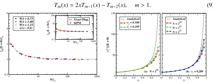
Figure 1. Left panel:Numerical study of the convergence of the localization length to its
thermody-namic limit value, i.e. plot ofξN(E =0)/ξ∞as a function ofN/ξ∞for the 1D Anderson model with
open boundaries. The data were computed using the KPM withM =2048 Chebyshev moments and
have an estimated error of 1%. The parameterξ∞is the analytically calculated localization length in
the perturbative regime forN→ ∞[8]. In the inset, we confirm the convergence of the KPM estimates of the localization length by comparing with the results calculated by an exact diagonalization of the disordered Hamiltonian forW/t=1.
Right panel:Estimates of the normalized localization lengthσ2εξ(E=0), as a function ofαfor the de
Moura-Lyra model with OBC using the KPM. The computations were carried out for a fixed(a)system of size ofN =218sites and various local variances,σε, and(b)σε=0.289 (i.e.W =t) and for various
system sizes. Once again,M=2048 Chebyshev moments were used to obtain an 1% estimated error
of convergence. The dashed black curve stands for the Izrailev-Krokhin result (Eq. (7)) and, in(b), the numerical curves seem to be converging towards this one asNis increased. This reflects the strong finite-size effects which are known to exist in this problem.
which starts withT0(x)=1 andT1(x)=x. Additionally, they also satisfy the orthogonality
relation
1
−1 Tn(x)Tm(x)(1−x
2)−1/2dx=π
2δn,m(δn,0+1). (10) Since Thouless’ result [6] expresses the inverse localization length in terms of a density of states, KPM estimates of the localization length may be obtained from the KPM approxi-mated density of states [1, 3] as: [4]
1
ξ(E) =−ln 2−2
M−1
m=1
µmgm
m Tm(E). (11)
While this allows the computation ofξ−1(E) for any band energyE, we will focus on the
band center without any loss of generality. The KPM moments in Eq. 11,µm, are defined as
µm = −11Tm()ρ()d= N1Tr[Tm( ˆH)]. (12)
The expression of Eq. (11) is the truncated series with M terms. This abrupt truncation introduces Gibbs oscillations—signaling non-uniform convergence. This numerical artifact can be filtered out of the final result by employing an optimized damping factor, such as the so-calledJackson Kernelgmdefined as [1]:
gm=(M−m+1) cos(
mπ
M+1)
M+1 +
sin( mπ
M+1) cot( π
M+1)
These polynomials obey the following recursion relation
Tm(x)=2xTm−1(x)−Tm−2(x), m>1. (9)
1 10 100 1000
N/ξ∞
0.5 1 2 4 8 ξN
(E = 0)/
ξ∞
W/t = 0.75 W/t = 1.00 W/t = 1.25 x/(x - 0.6)
1 10 100 1000
0.1 1 10 100
ξN
(E = 0)/
ξ∞ Exact Diag. KPM
N/ξ∞
0 0.2 0.4 0.6 0.8 1
α 0 50 100 150 σε
2ξ(E = 0)
Analytical
σε = 0.500
σε = 0.289
0 0.2 0.4 0.6 0.8 1
α
Analytical N = 218
N = 222
N = 225
(a) N = 218 (b) σε = 0.289
Figure 1. Left panel: Numerical study of the convergence of the localization length to its
thermody-namic limit value, i.e. plot ofξN(E =0)/ξ∞as a function ofN/ξ∞for the 1D Anderson model with
open boundaries. The data were computed using the KPM withM =2048 Chebyshev moments and
have an estimated error of 1%. The parameterξ∞is the analytically calculated localization length in
the perturbative regime forN→ ∞[8]. In the inset, we confirm the convergence of the KPM estimates of the localization length by comparing with the results calculated by an exact diagonalization of the disordered Hamiltonian forW/t=1.
Right panel:Estimates of the normalized localization lengthσ2εξ(E=0), as a function ofαfor the de
Moura-Lyra model with OBC using the KPM. The computations were carried out for a fixed(a)system of size ofN =218sites and various local variances,σε, and(b)σε =0.289 (i.e.W =t) and for various
system sizes. Once again,M=2048 Chebyshev moments were used to obtain an 1% estimated error
of convergence. The dashed black curve stands for the Izrailev-Krokhin result (Eq. (7)) and, in(b), the numerical curves seem to be converging towards this one asNis increased. This reflects the strong finite-size effects which are known to exist in this problem.
which starts withT0(x)=1 andT1(x)= x. Additionally, they also satisfy the orthogonality
relation
1
−1 Tn(x)Tm(x)(1−x
2)−1/2dx=π
2δn,m(δn,0+1). (10) Since Thouless’ result [6] expresses the inverse localization length in terms of a density of states, KPM estimates of the localization length may be obtained from the KPM approxi-mated density of states [1, 3] as: [4]
1
ξ(E) =−ln 2−2
M−1
m=1
µmgm
m Tm(E). (11)
While this allows the computation ofξ−1(E) for any band energyE, we will focus on the
band center without any loss of generality. The KPM moments in Eq. 11,µm, are defined as
µm = −11Tm()ρ()d=N1Tr[Tm( ˆH)]. (12)
The expression of Eq. (11) is the truncated series with M terms. This abrupt truncation introduces Gibbs oscillations—signaling non-uniform convergence. This numerical artifact can be filtered out of the final result by employing an optimized damping factor, such as the so-calledJackson Kernelgmdefined as [1]:
gm= (M−m+1) cos(
mπ
M+1)
M+1 +
sin( mπ
M+1) cot( π
M+1)
M+1 . (13)
0 0.2 0.4 0.6 0.8 1
DN(α, 1)
0 20 40 60 80 100 σε 2ξ
(E = 0)
N = 218
N = 220
N = 222
N = 225
y = axb
0 0.2 0.4 0.6 0.8 1
α 4 16 64 256 1024 Analytical Extrapolations
(a) (b)
Figure 2. (a)Plot of the normalized localization length,σ2εξ(E =0), as a function of the parameter
DN(α,1), for the de Moura-Lyra model with OBC at zero temperature. The numerical computations
were carried out for a disorder varianceσε = 0.289 using M = 2048 Chebyshev moments and an
estimated error of 1%. The data can be collapsed into a single curvey=axb(dashed magenta line).(b)
Comparison between the thermodynamic limit values ofσ2εξ(E =0) predicted by the dashed curve in
(b), with the analytical expression of Eq. (7).
4 Results and Discussion
In order to validate our KPM estimates ofξ−1, we first addressed the numerical convergence
of the localization length for the well-known uncorrelated Anderson model. In the left panel of Fig. 1, we illustrate the convergence of our finite lattice results towards the perturbative thermodynamic limit result (ξ=105.2/W2) as the size of the chain is increased, for different
disorder strengths. All the calculations were done with an estimated error of 1% as deter-mined by the standard-deviation of the sample-specific fluctuations in the localization length. In addition, we found the numerical data of Fig. 1 to be well fitted to the scaling function,
ξ(E=0)
ξ∞ =
x
x−x0, x0∼0.6. (14)
wherex=N/ξ∞.
The delocalization behavior of the eigenstates in the de Moura-Lyra potential is illustrated in Fig. 1 (right panel). The rescaled localization length shows large deviation from Izrailev’s result forσε=0.5 (non-perturbative regime). However, it starts to converge with decreasing
σεfor a fixed-system size as signaled by the approaching curves in(a). Nevertheless, there are strong system finite-size effects [12], clearly visible in (b), which prevent the observation of a fully converged curve for sizes as large asN =225sites. The convergence is then very slow near the transition pointα∼1.
an excellent agreement with the analytical result, thus confirming the delocalization transition atα=1 found earlier by the authors.
5 Conclusions
We reported numerical calculations of the localization length in one-dimensional disordered tight-binding models with uncorrelated (Anderson model) and also spatially correlated (de Moura-Lyra model) on-site disorder. The calculations were done by applying the very ef-ficient Kernel Polynomial Method to implement the Thouless formula for the localization length of a general one-dimensional tight-binding model with open boundaries.
For the Anderson model, we found an excellent agreement of the KPM-estimated local-ization length with the perturbative analytical results, confirming the validity of our proce-dure. We also studied the dependence of the measuredξwith the chain’s size, thus checking
its convergence to the well-known value in the thermodynamic limit.
For the trickier de Moura-Lyra model, we showed that our KPM implementation of the Thouless formula fully confirms results obtained previously with Landauer formal-ism.Namely, we were able to reproduce the divergent behavior of the localization length ,
ξ ∝ (1 −α)−1, in the vicinity of delocalization transition at “α = 1”, in the perturbative regime. This observation was done by a finite-size extrapolation similar to the one used by Santos Pireset al[12].
Acknowledgments:
For this work, N.A. Khan was supported by the INTERWEAVE project, Erasmus Mundus Action 2 Strand 1 Lot 11, EACEA/42/11 Grant Agreement 2013-2538/001-001 EM Ac-tion 2 Partnership Asia-Europe and J. P. Santos Pires was supported by the MAP-fis PhD grant PD/BD/142774/2018 of Fundação da Ciência e Tecnologia. The authors also acknowl-edge financing from Fundação da Ciência e Tecnologia and COMPETE 2020 program in FEDER component (European Union), through the projects POCI-01-0145- FEDER-028887 and UID/FIS/04650/2013.
References
[1] A. Weiße, G. Wellein, A. Alvermann, and H. Fehske, Rev. Mod. Phys., 78:275 (2006). [2] F. Lacopi, J. J. Boeckl, and C. Jagadish,2D Material(Academic Press, 2016)
[3] R. N. Silver, H. Roeder, A. F. Voter, and J. D. Kress, J. Comput. Phys. 124:1 (1996). [4] N. Hatano and J. Feinberg. Phys. Rev. E, 94:063305 (2016).
[5] N. A. Khan, J. M. Viana Parente Lopes, J. P. Santos Pires, and J. M. B. Lopes dos Santos. J. Phys.: Condens. Matter, 31:175501 (2019).
[6] D. J. Thouless. J. Phys. C: Solid State Phys., 5:77 (1972).
[7] D. J. Thouless.III-Condensed Matter, Les Houches Session XXXI. (North-Holland, New York, 1979).
[8] F. M. Izrailev, A. A. Krokhin, and N. M. Makarov. Phys. Rep., 512:125 (2012). [9] P. A. Lee and T. V. Ramakrishnan. Rev. Mod. Phys., 57:287 (1985).
[10] F. A. B. F. de Moura and M. L. Lyra. Phys. Rev. Lett., 81:3735 (1998) [11] G. M. Petersen and N. Sandler. Phys. Rev. B, 87:195443 (2013).
[12] J. P. Santos Pires, N. A. Khan, J. M. Viana Parente Lopes, and J. M. B. Lopes dos Santos. Phys. Rev. B, 99:205148 (2019).
[13] F. M. Izrailev and A. A. Krokhin. Phys. Rev. Lett., 82:4062 (1999).