Article
The Role of Respiration in Estimation of Net Carbon
Cycle: Coupling Soil Carbon Dynamics and Canopy
Turnover in a Novel Version of 3D-CMCC Forest
Ecosystem Model
Sergio Marconi1,2*, Tommaso Chiti3,4, Angelo Nolè 5, Riccardo Valentini2,4, Alessio Collalti 2,6
1. School of Natural Resources and Environment, Institute of Food and Agricultural Sciences, University of Florida (UFL), Gainesville, US: [email protected]
2. Foundation Euro-Mediterranean Center on Climate Change– Impacts on Agriculture, Forest and Ecosystem Services (IAFES), 01100 Viterbo (VT), Italy;
3. University of Tuscia – Department for Innovation in Biological, Agro-Food and Forest Systems (DIBAF), Viterbo, VT, Italy
4. Far Eastern Federal University (FEFU), Ajax St., Vladivostok, Russky Island, Russia
5. School of Agricultural, Forestry, Food and Environmental Sciences (SAFE), University of Basilicata, Italy
6. CNR-ISAFOM National Research Council of Italy, Institute for Agriculture and Forestry Systems in the Mediterranean, 87036, Rende, CS, Italy
*Correspondence: [email protected]; Tel.: +1-352-745-9685
Abstract: Understanding the dynamics of Organic Carbon mineralization is fundamental in forecasting biosphere to atmosphere Net Carbon Ecosystem Exchange (NEE). With this perspective, we developed 3D-CMCC-PSM, a new version of the hybrid Process Based Model 3D-CMCC FEM where also heterotrophic respiration (Rh) is explicitly simulated. The aim was to quantify NEE as a forward problem, by subtracting Ecosystem Respiration (Reco) to Gross Primary Productivity (GPP). To do so, we developed a simplification of the Soil Carbon dynamics routine proposed in DNDC [1]. The method calculates decomposition as a function of soil moisture, temperature, state of the organic compartments, and relative abundance of microbial pools. Given the pulse dynamics of soil respiration, we introduced modifications in some of the principal constitutive relations involved in phenology and littering sub-routines. We quantified the model structure related uncertainty in NEE, by running our training simulations over 1000 random parameter-sets extracted from parameters distributions expected from literature. 3D-CMCC-PSM predictability was tested on independent time series for 6 Fluxnet sites. The model resulted in daily and monthly estimations highly consistent with the observed time series. It showed lower predictability in Mediterranean ecosystems, suggesting that it may need further improvements in addressing evapotranspiration and water dynamics.
Keywords: Forest ecosystem; Fluxnet; Soil respiration; Net ecosystem Exchange; Phenology
1. Introduction
Global concerns over increasing level of greenhouse gas concentration, particularly carbon dioxide (CO2), pushed research efforts to better investigate biogeochemical Carbon (C) fluxes dynamics and patterns between atmosphere and biosphere, and to upscale C flux estimates from site-specific to regional, continental and global scales. Increased atmospheric concentration of CO2, combined with increasing temperatures and size variations of ecosystem C pools, are responsible for year-to-year terrestrial ecosystems carbon flux perturbations, through the variation of both photosynthetic and respiration rates [2].
In the last decades, the Eddy Covariance (EC) technique provided long-term continuous measurements of Net Carbon Ecosystem Exchange (NEE), water vapor and energy, within the global network of EC flux towers (FLUXNET) distributed over major terrestrial ecosystems. The availability of EC measure of NEE contributed to quantify and to determine seasonal and inter-annual variability of ecosystem C budgets at EC tower site-specific scale [3; 4; 5]. Observed NEE does not directly quantify the two major components of ecosystem C flux balance represented by ecosystem respiration (Reco) and gross primary productivity (GPP). Thus, flux partitioning algorithms have been developed to partition eddy covariance NEE into photosynthetic uptake and respiratory release [6; 7]. At the same time, EC flux measurements provide key information for the parameterization, calibration and validation of process-based Forest Ecosystem Models (FEMs) contributing to large scale estimates of main ecosystem C pools.
The implementation of both forest process-based models (PBMs) [8; 9; 10; 11; 12; 13] and Functional–Structural Tree Models (FSTMs) [14; 15; 16; 17], based on the widely used Light Use Efficiency (LUE) approach [18], contributed to understand and up-scale the the main physiological processes supporting ecosystem's C uptake. Although most of forest ecosystem models provide reliable estimates of forest growth, limitation for NEE estimates are related to the uncertainty in Reco estimation [19; 20]. Hence, the implementation of biogeochemical models integrating soil respiration models and FSTMs is a great opportunity to reliably estimate NEE [21; 22; 23].
Although soil respiration and soil organic matter (SOM) decomposition depend mainly on abiotic factors, such as temperature and soil moisture [24; 25; 26], a key role is played by soil organic carbon (SOC) stock size, microbial pools [27; 28], and dynamics of SOC supply to soil with littering [29]. Leaf and fine roots senescence is of primary importance in determining dynamics in heterotrophic respiration [30; 31], and exhibits seasonal patterns and intra seasonal pulses [32; 33]. These pulses are mostly driven by phenological transitions through stages of dormancy, active growth, and senescence. For example, supply of dead leaves in soil is strongly dependent to tree’s leaffal strategy. This is also true when predicting tree respiration, which is directly related to their growth and Nitrogen content, which depends on Spring phenology. Unfortunately, processes involving budburst and senescence are still partly obscure. PBMs usually represent these processes simplistically: these simplifications may lead terrestrial ecosystem models to overly result in biased predictions [34; 35; 36].
For these reasons, we developed the 3D-CMCC-PSM (3D-CMCC-Phenology and Soil Model), a new version of the hybrid Process-Based Model 3D-CMCC FEM proposed by Collalti et al. [37; 38], where 1) Spring phenology was directly taking into account tradeoffs between growth and Non Structural Carbon (NSC) demand; 2) phenological transitions and supply of Fresh Organic Matter (FOM) to soil were more explicitly represented; and 3) heterotrophic respiration (Rh) was explicitly simulated to dynamically quantify stock changes of 7 different SOC pools mediated by the amount of active microbial C pools. The aim of this study was to: 1) test the performance of the modified model version, comparing model NEE estimates against independent time series for 6 Fluxnet sites, representing different forests in different climatic areas, distributed over a wide latitudinal gradient amongst European EC sites; 2) quantify uncertainty associated to 3D-CMCC-PSM constitutive relations structure and parameterization.
2. Materials and Methods
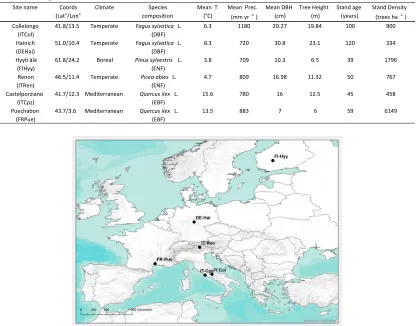
2.1. Study Area and data
dominated by different species composition from deciduous broadleaved, DBF (i.e. Fagus sylvatica L.), evergreen broadleaved, EBF (i.e. Quercus ilex L.), and evergreen needle leaved, ENF (i.e. Pinus sylvestris L. and Picea abies L.), representing the most common European forest species from Boreal to Mediterranean Ecoregions across Europe.
Table 1. Sites description and stand initialization data. Mean Temperature (T) and Precipitation (prec.) are
annual averages collected at site.
Figure 1. Location of the 6 Fluxnet sites used to evaluate 3D-CMCC-PSM.
2.2 Model description
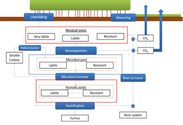
The 3D-CMCC FEM is a stand-scale process-based model (PBM) designed to simulate C and water cycle in natural and managed forest ecosystems (for a full description see [37; 38]). Several eco-physiological processes were modeled at species-specific level, and at a variable temporal scale (from daily to annual) depending on the process to simulate (Figure 2). Model outputs were generally represented at hectare scale, while processes were simulated at different spatial scales from cellular (e.g. stomatal conductance), to canopy (e.g. transpiration), to individual tree, up to stand level.
Carbon assimilation was modeled for sun and shaded leaves [1] using the LUE approach [42]: potential C assimilation was constrained by environmental and stand structural (e.g. tree age) scalars [43]. Autotrophic respiration (RA) was explicitly modeled as the sum of growth and maintenance respiration (RG and RM, respectively). The first was computed as a fixed ratio of new growth tissues (30%) the latter was based on Nitrogen content in stems, branches, leaves, fine and coarse roots, non-structural carbon (NSC), and fruits tree pools. Carbon allocation among these pools was controlled by species-specific parameters, phenology, light and water availability. Water cycle was modeled calculating the daily balance between precipitation, canopy transpiration, evaporation, soil evaporation, and runoff. Meteorological variables used to force the model were: global solar radiation (MJ m-2 day-1), maximum and minimum air temperature (°C), relative humidity (%), and daily
Sitename Coords (Lat°/Lon°
)
Climate Species
composition
Mean T (°C)
Mean Prec. (mmyr-1)
MeanDBH (cm) TreeHeight (m) Standage (years) StandDensity (treesha-1) Collelongo
(ITCol)
41.8/13.5 Temperate Fagus sylvatica L. (DBF)
6.3 1180 20.27 19.84 100 900
Hainich (DEHai)
51.0/10.4 Temperate Fagus sylvatica L. (DBF)
8.3 720 30.8 23.1 120 334
Hyyti älä (FIHyy)
61.8/24.2 Boreal Pinus sylvestris L. (ENF)
3.8 709 10.3 6.5 39 1796
Renon (ITRen)
46.5/11.4 Temperate Picea abies L. (ENF)
4.7 809 16.98 11.32 50 767
Castelporziano (ITCpz)
41.7/12.3 Mediterranean Quercus ilex L. (EBF)
15.6 780 16 12.5 45 458
Puechabon (FRPue)
43.7/3.6 Mediterranean Quercus ilex L. (EBF)
cumulated precipitation (mm day-1). To be initialized model required knowing stand structural characteristics such as: species composition, stand density, diameter at breast height (DBH), tree height and age. Soil initialization required the estimation of Total Organic Carbon (TOC) in the different SOC pools, as described in the following section.
Figure 2. 3D-CMCC version PSM main flowchart modified from Collalti et al., 2014. Red circled boxes represent
the pools and variable introduced or modified by 3D-CMCC-PSM.
2.2. Model Improvements 2.2.1. Soil Carbon Dynamics
The most recent 3D-CMC FEM model version (v.5.1, [38]) lacks in representing SOC dynamics, preventing any estimation of NEE. With that perspective, we developed a simplified version of the method described in [1] to quantify, dynamically, changes of 7 different SOC pools mediated by the amount of active microbial C pool (Figure 3).
Figure 3. Soil Carbon dynamics in 3D-CMCC-PSM. The three macro pools are highlited by red boxes (dead C
pool) and blue box (live C pool, i.e. microbial). Blue filled boxes represent the processes simulated by the soil
model.
transformed in other organic compounds [1]. SOC stability is also related to its chemical recalcitrance, its accessibility, and interaction with clays [44]. We divided SOC in 7 pools to take these differences into account. Humic pool (we use the term Humads, to be consistent with [1]) was divided into a more labile (labile Humads, which stands for Humic acid), an intermediate (resistant Humads, which stands for Fulvic acid) and a more resistant sub-pool (Humus, which stands for Humine).
We assumed that microbial C use efficiency was different for different pools, but constant within each pool [42]. Microbial activity is strictly related to micro-environmental conditions too. Given these premises we modeled C dynamics among soil pools using the following two partial differential equations:
= ( ) − ( ) ( )
= ( ) ( ) − α ( ) , (1)
with being the CO2 efflux produced from a specific C pool decomposition, ( ) is the amount of new Carbon entering the specific soil pool, ( ) the amount of Carbon in that C pool, ( ) the microbial biomass competing for ( ). α and β respectively represented the microbial turnover and SOM consumption factors. α was treated as a constant value, as in [1].
The consumption factor β was estimated as a function of both SOM stability and micro-environmental conditions:
=
= −0.014 + 0.099 + 0.02
= −2.85 + 1.49 + 1.77 − 0.03
= 0.6 . (−0.02
%+ 0.03)
= . %
. + 1
, (2)
where represented the temperature factor, the moisture factor, the accessibility, the recalcitrance; a clay dependent depth factor [45]. The factor was treated as a specific parameter depending on each compartment’s biomass. represented Temperature in Celsius degrees, θ stands for water moisture, z the mean depth of the soil, % is the percentage of clays
in soil.
Humads were decomposed using the same rationale, but slower rates. Inert Organic Matter (IOM) was calculated following [46].
2.2.2. Deciduous Phenology
Similarly to [38] the phenology scheme was constrained in 3 and 5 sub-phases respectively for evergreen and deciduous species (Table 2). These phases were driven by photoperiod, thermal sum, and maximum leaf biomass (resulting from maximum attainable Leaf Area Index, LAI, m2 m-2).
Table 2. Description of the different phenological phases for deciduous and evergreen species used in 3D-CMCC
PSM.
We based the tradeoff function on the hypothesis that new leaves demand of NSC is higher during budburst, and gets progressively lower when maturing [48]. Idealistically, the total NSC mass
(B ) demanded by maturing shoots and leaves could be represented by the linear differential equation (ODE):
− R (t) ∙ B (t) = 0, (3)
where R (t) is the instantaneous proportion of NSC demand. We assumed that C request per leaf exponentially decreases with maturity, while the total demand increases by the increasing number of leaf primordia. For simplicity, we assumed that the two components resulted in the linear reduction of R (t). Being a fraction, the maximum value of the integral of R & & (t) is equal to 1.
Being the first vegetative day t0, and the last day of Budburst (BB ) the last possible one to reach complete leaf development, the domain of the function was [t0, BB ]:
1 = ∙ δt → R = → R (t) = , (4)
resolving the ODE, and substituting R & & (t) it gives:
B (t) = ∙ ∙ , (5)
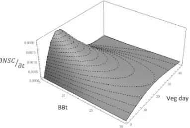
where BB is the parameter used in [38], e is the biomass dependent and e ⁄ the maturity dependent factors (expressed in days). Graphically, the equation represents a skewed function of the amount of NSC allowed to be used by the trees of the specific class; the faster the leaves reach maturity, the more daily specific allocation is allowed (Figure 4).
Figure 4. Graphic representation of the C tradeoff function. The axes represent respectively bud burst days (BBt),
vegetative days (Veg_day), and the fraction of total NSC invested in leaves development ( ). The shorter
BBt, the highet the maximum NSC fraction.
Phase
Trigger
Phase
Trigger
Bud
Burst
GDD
threshold
Bud
Burst
GDD
treshold
Leaf
Development
PeakLai/2
PeakLai
Pipe
Model
PeakLai
Pipe
Model
Leaffall
Daylength
Treshold
Leaffall
Daylength
Treshold
Unvegetative
Delpierre
et
al.,
2012
Another major modification we introduced involves Fall leaf yellowing and senescence. Falling leaves contribute to half of annual litter production. Correctly estimate their timing have strong impact on both GPP and Rh dynamics [33]. The 5.1 version of 3D-CMCC-FEM represents senescence by linearly decreasing leaves biomass of a predefined fraction until their pool is emptied. However, such method systematically overestimated leaf turnover at the beginning of the Leaffall phase, and is poorly flexible in calculating its duration. For these reasons, linear loss of leaf Biomass was replaced with a sigmoid function. Assuming for hypothesis that all leaves fall by the end of senescence season, the sigmoid function was:
= LAI(t) − Max 0, ( , , )( )
( ) , (6)
Where α(t), β(t), γ(t) are three parameters with biological or physical meaning. In fact:
(ℎ, , ) = (ℎ, , )
( ) = ( ) +∆ ( )
( ) ≅ ( . ) ∆ ( )( ( ( ) . ))
, (7)
where L stands for LAI value at peak of green, t (s) is the first day of senescence (triggered by a species-specific day-length parameter), ∆t(s) is the length of the senescence period (days). ∆t(s) was calculated using [49], as a function of Temperature and photoperiod:
R (t) = (T (s) − T(t)) ∙ ( )( )
∆t(s) = ∑ ( )( ) R (t)
, (8)
where TMax is the maximum temperature at which senescence is effective, T(t) is daily average Temperature, D (0) photoperiod at the first day of senescence , D (t) photoperiod at the ith day of the year.
2.2.3. Evergreen Phenology
Evergreen canopy turnover was modified from [38]. 3D-CMCCFEM v.5.1 assumes that evergreen leaf turnover is constant throughout the year, and that annual leaf turnover is equal to leaf biomass produced the year before [38; 47]. However, leaf turnover seems to be concentrated in specific seasonal windows: 1) consistently to leaf emergence (Spring); and 2) approaching of photosynthetic inefficient season (Fall) (Devi et al., 2013; Chabot et al., 1982; Nitta et al., 1997). For this reason, this approach may affect the ability in estimating leaf biomass and GPP intra-annual variability. To better represent leaf turnover dynamics, we developed a new framework where competition for light dynamically affected leaves turnover. We assumed the canopy to be a population of leaves optimized to intercept the highest amount of light. Since leaves cannot move from their position in the canopy, they get partially shaded by new emergent leaves when aging. Conceptually, leaves can be assumed to be in competition for one resource, light, and their turnover can be predicted by using a competition for one resource scheme as in [50]:
( )B (t) = f (R) − f (m )
f (R) = ( ∙ )
R∗= ∙
( )
, (9)
In this model, R and R∗ are respectively the concentration of available light in J m-2 d-1 (i.e. resource that leaves are competing for), and the light needed to survive in a progressively more shaded canopy. r is the max photosynthetic rate (gC m-2 d-1), m is the Maintenance Respiration in gC m-2 d-1, Y Carbon yield.
(1) Older leaves live in the shaded portions of the canopy, where light transmitted is reduced following Lambert Beer’s exponential decay equation. For this reason, we expect an exponential reduction in absorbed photosynthetically active radiation (APAR);
(2) An age dependent quasi exponential decay in leaf quantum yield efficiency [51]. These decays impact on the reduction of r;
(3) Nitrogen content in older leaves is often lower than in young ones, because of its transfer from portions of the crown with low productivity to portions more exposed to light [51]. Since Maintenance respiration is proportional to Nitrogen content, we expect an exponential reduction in ;
(4) Y was assumed to be constant as in [52] because of the joint effect of reduction in respiration rate and quantum yield efficiency.
We assumed that the three components of the Eq.9 may have the following shapes:
m = m ∙ e ∙ + m
r = α ∙ e ∙ + α ∙ λ ∙ e ∙ + λ
k
, (10)
where t is time, the independent variable. m , α , λ are MR, quantum yield and APAR at first day of budburst, the second year of life. m , α , λ are the theoretical minima values of MR, quantum yield and APAR to let a proportion of leaves survive in a non-shading context. k , k , k are the exponential parameters for the three functions.
Based on these hypotheses Eq 10. becomes:
R∗= ∙ ∙ ∙
∙ ∙ ∙ ∙ ∙ ∙ ∙ , (11)
Assuming that k = k = k , and that the denominator of Eq. 9 has to be greater than zero for the leaves in the ith generation to survive, R* is a sigmoid positive function.
Knowing R*, we can calculate the amount of live leaf biomass of the ith generation ( ( )) as the inversion of R* (i.e. S∗(t)). We simplified the theoretical model using the following function:
S∗(t) = t − ( ) t + BF
( ), (12)
where t is the number of days since leaves of the ith generation have emerged. According to this model the theoretical maximum age of each generation (BF ( )) should correspond to the year in which the
R* almost reaches its asymptote. We used Eq. 12 to quantify leaf turnover for each generation. About 60% of leaf turnover happened in early Spring, when new leaves emerged: the amount of biomass lost every day was proportional to new leaf biomass production the same day. The rest of annual turnover happened in Fall, when each leaf biomass generation was reduced of a constant value calculated from Eq. 12. No foliar re-sprouting was simulated in Fall, even though there are evidences of it for Quercus ilex [53]. Leaf biomass reduction was determined by linearly decreasing each Bi to the quantity predicted by the specific parabolic decay for the end of the year.
2.2.4 Production of Fresh Organic Matter
= ∙
= −
< <
, (13)
Where C is the FOM entering litter from each structural C compartments of the plant. FOM C and N were distributed to the litter sub pools with closest C:N. C , represents the pool with higher recalcitrance. When CN was higher than any litter sub pool, all the new C was added to the structural resistant pool; otherwise, if CN was lower than the CN of the metabolic pool, all its C and N were added to the very labile sub pool. Litter C dynamically moved from a pool to another. Microbes absorbed and partially immobilized litter C in their biomass, and released it again in the soil, during the humification processes [56].
2.2.5. Optimization
We introduced a new calibration scheme to provide an optimized parameterization, and quantify uncertainty related to the equations used in 3D-CMCC-PSM to simulate NEE, and choice of a subset of 45 species-specific physiological parameters (Table S1). Calibration was performed on each site independently, using a training dataset composed by 3 years of EC daily NEE time-series. We chose 2000-02 for DEHai, 2001-03 for FIHyy, ITCpz, and FRPue; 2001-04 for ITCol; 2006-2008 for ITRen. Because of the strong autocorrelation characterizing time-series, we didn’t randomly split our dataset, and decided to use sub-time series of contiguous years [57]. We preferred to use the beginning of each simulation for training, before the global recession following the Financial Crisis of 2007-2008. We decided to do so to (1) facilitate comparison among different sites’ simulations; (2) have the calibration start when vegetation structure was known from literature, and (3) reduce the risk for parameters to be fitted over a changing environment instead of eco-physiological properties.
To sample the parameterization space (the realistic values of each physiological parameter of the species simulated in each site), we randomly extracted 1,000 parameter-set combinations from prior distributions. Prior distributions were assumed to be the same among individuals of the same species, different across species. We assumed each parameter to follow a truncated normal distribution, to avoid any possibility to have non-realistic negative values. Average and variance were estimated by using values found in literature, as in [38]. We used the same averaged value as in [38] for those parameters whose observations in literature were less than 3, because we didn’t have enough information to calculate sample standard deviation. The optimization was performed by choosing the parameterization set maximizing the objective function QF through:
QF = ∑ ∙ −
∑ ∙∑
∑ 2−∑
2
∑ 2−∑
2 × 1 −
∑ − 2
∑ − 2 , (14)
where YObs represents EC daily NEE, Ysim Modeled NEE for the same day, the average EC daily NEE over the train time series. The first part of the RHS of the equation represents the square of the Pearson Correlation coefficient (R), the second the Nash-Sutcliffe Efficiency index (NSE).
2.2.6. Validation Analysis
To evaluate the model efficiency, we calculated daily, monthly, and seasonal: (1) R; (2) NSE; (3) Root mean square error (RMSE); and (4) Mean Absolute Bias (MAB). Each statistic was considered differently informative [58] as summarized in Table 3. The model’s ability in representing observed anomalies was determined by analyzing inter annual variability (IAVs) following [59] and [38].
Table 3. Statistics used for Model’s results validation against Eddy Covariance data.
3. Results
3.1. Evaluation of daily, seasonal, and annual NEE estimations
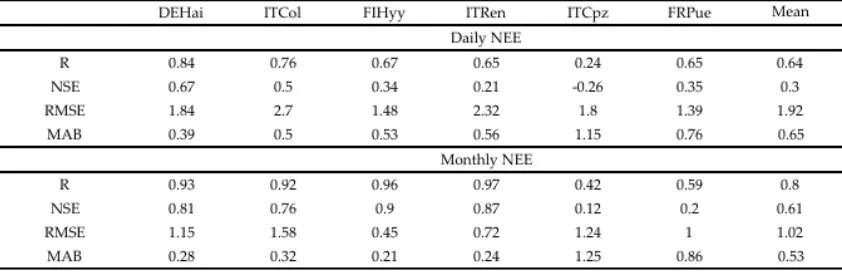
To evaluate 3D-CMCC-PSM NEE predictions, we compared predicted (MD) daily and monthly NEE time series to EC daily data. The analyses were performed only on the test data (i.e. portions of the series which have not been used for calibration) to avoid any effect of overfitting. The model showed high correlations with observed EC data at all sites for both daily and monthly fluxes, apart from ITCpz site (Table 4). Excluding ITCpz, R ranged at all sites from 0.65 to 0.84 for daily and, 0.59 to 0.97 for monthly scale. Beech dominated Deciduous Forests (DBF) performed better than Conifer species (ENF) and evergreen Mediterranean broadleaved forests (EBF). ENF and EBF in FRPue performed similarly on daily scale, for all the statistics used. However, ENF predictability significantly increased on monthly scale (R ranging between 0.92 and 0.97), while EBF performed worse (R 0.42 in ITCpz, and 0.59 in FRPue). RMSE on average was 1.92 gC m-2 d-1. MAE ranged between 0.96 and 1.78 gC m-2 d-1, and on average it decreased almost twice on monthly timescale. MAB showed similar behavior for DBF and ENF. It ranged between 0.39 and 0.56 gC m-2 d-1 (0.50 on average) for daily time series. Mediterranean forests resulted the ones with highest MAB, and showed no significant reduction when predictions were aggregated on monthly scale. Differently from the other simulations, even NSE just improved slightly for ITCpz, and even reduced for FRPue simulation.
Table 4. Daily and Monthly Validation statistics calculated on the test-set. As stated in Table 3, R and NSE are
dimensionless; RMSE and MAB are gC m-2 d-1.
Statistics Formulation Use and ranges
Pearson Coefficient Estimation of model’s measure of correlation with EC data [0;1]
Nash Sutcliffe efficiency Estimation of model’s predictability [-∞;1]
Root M ean Square Error Estimation of model’s accuracy gC m-2 d-1 [0; ∞]
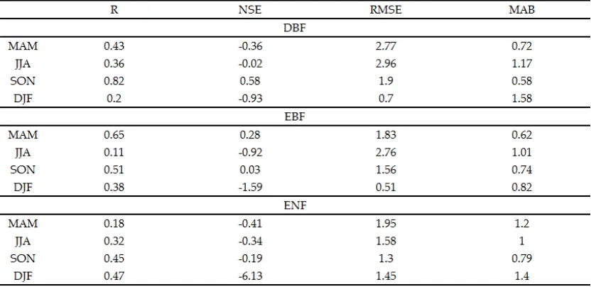
Daily results were aggregated in seasonal series to evaluate seasonal predictability. Daily NEE were averaged to give a time series of mean seasonal NEE (gC m-2 d-1), one value per season, for the duration of the test dataset. Seasonal aggregations showed that 3D-CMCC-PSM poorly performed in predicting seasonal fluxes. NSE was generally negative in Summer, with the exclusion of DEHai and FRPue. 3D-CMCC-PSM generally best reproduced NEE dynamics in Fall (R ranging between 0.22 and 0.89). ENF ecosystems showed consistently higher correlation in Spring predictions, with R of 0.65 and MAB of 0.62 gC m-2 d-1 on average. In the case of evergreen stands, 3D-CMCC-PSM consistently showed poor performance in Summer. Expectedly, DBF performed the worst in Winter (Table 4). NSE on average resulted positive only in Fall for both DBF and EBF, and Spring, for ENF stands.
Table 5. Seasonal validation statistics calculated on the test-sets and aggregated by ecosystem type. As stated in
Table 3 and 4, R and NSE are dimensionless; RMSE and MAB are gC m-2 d-1. MAM stands for March, April, and
May. JJA stands for June, July, and August. SON stands for September, October, and November. DJF stands for
December, January, and February. DBF stands for Deciduous Broadleaf Forests, EBF for Evergreen Broadleaf
Forests, ENF for Evergreen Needle leaf Forests.
Figure 5. Taylor diagram representing 3D-CMCC-PSM performance in (a) daily, (b) monthly and (c) annual NEE
estimation for the test-set. ITCol and DEHai represent DBF (red and green dots); ITRen and FIHyy ENF (blue
and turquoise). ITCpz and FRPue represent EBF (yellow and magenta dots). The closest a simulation lied to the
“Ref” point, the better 3D-CMCC-PSM represented NEE patterns. X and y- axes represent NEE standard
deviation (SD): the closest to 1, the better the performance. Simulations with R ≥ 0.9, and difference in SD with
EC NEE less than 0.5 5 gC m-2 d-1 showed very good performance. Simulations with 0.75 ≤ R < 0.9, and
difference in SD with EC NEE between 0.5 and 1 gC m-2 d-1 showed good performance. Simulations with 0.35 ≤
R < 0.75, and difference in SD with EC NEE between 1 and 1.5 gC m-2 d-1 showed sufficiently good performance.
3.2. Anomalies and parameters related uncertainty
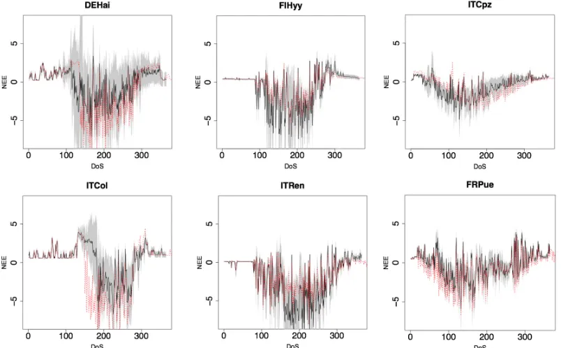
Figure 6 shows uncertainty associated to random choice of parameters. Overall, uncertainty was expectedly higher in Summer and Fall. Such increase was particularly clear for deciduous forests, which not only showed wider NEE standard deviation, but also had optimal modeled NEE falling outside standard deviation area.
Figure 6. Model structure related uncertainty in estimating NEE (gC m-2 d-1 ) per DoS (Day of Simulation) by a
randomly extracted parameterization-sets. Average daily simulations (black line) and standard deviation (grey
area). Red dotted line represents daily NEE simulation for the optimized parameterization set (Table S2). First
column represents DBF sites, the second ENF, the third EBF.
DBF sites showed also high uncertainty in estimating the first vegetative day, suggesting that a better representation of Winter dormancy effects on budburst dates may significantly improve model’s predictability. Uncertainty was generally lower in Mediterranean sites, probably because model’s performance was generally lower, and fitting parameters to data would have little effect on performance. 3D-CMCC-PSM uncertainty was generally low for ENF for most of the year, but was generally high when Temperature were higher. Higher uncertainty for warmer days was generally found in DBF sites too, suggesting that 3D-CMCC-PSM was expectedly sensitive to high Temperatures for both Photosynthesis [61] and Respiration [62]; because of such variability, calibrating parameters on data resulted in a significant boost in model’s predictions.
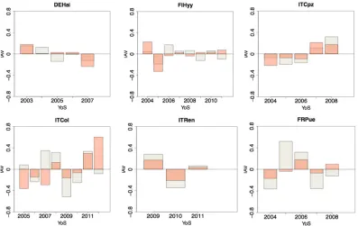
NEE inter-annual variability was generally underestimated by the model. Nevertheless, 3D-CMCC-PSM correctly reproduced 81% of the sign of the anomalies, and residuals difference in magnitude was usually less than 0.3 gC m-2 d-1. Highest difference in magnitude occurred in ITCol (difference in residuals higher than 0.5 gC m-2 d-1 in 5 years out of 12). Highest difference was shown in ITCpz, where the sign was correctly reproduced only once out of 8 years, and having more than 1gC m-2 d-1 of residual difference (Figure 7).
Figure 7. Inter annual variability (IAV) for the test time-series (gC m-2 month-1). Observed IAV in gray boxes,
simulated IAV in orange. First column represents DBF sites, the second ENF, the third EBF.
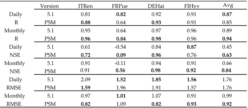
3.3. Comparison with the 5.1 version of 3D-CMCC-FEM
Daily NSE too was generally higher in 3D-CMCC-PSM, except for FlHyy. Monthly aggregated predictions were consistently outperforming those of 3D-CMCC-FEM 5.1 (Table 6).
Table 6. Comparison between 3D-CMCC-FEM 5.1 (5.1) and 3D-CMCC-PSM (PSM) versions, using the same
parameterization for 4 out of 6 sites (ITRen, FRPue, DEHai, FIHyy). As stated in Table 3, R and NSE are
dimensionless; RMSE is gC m-2 d-1. Bold values represent best performing version.
3.4. Daily and monthly Reco
We evaluated Reco by comparing modeled (MD) and observed (EC) daily and monthly time series. Daily R ranged between 0.45 in ITCpz and 0.9 in FIHyy (Table 7) . RMSE was of 1.28 gC m-2 d-1 on average, and MEB ranged between 0.43 and 1 gC m-2 d-1. Most of the bias happened in summer, where Reco was generally overestimated, especially in ITCol and ITCpz. NSE was positive in any case but ITCpz. It was generally lower in DBF (0.32), and higher in FIHyy (0.60) and FRPue (0.57). Reco at monthly timescale was strongly improved in predictability, especially for ITRen, whose R increased to 0.67 and NSE to 0.84. Montlhy predictions showed improvements for the other simulations too, improving R and NSE of about 0.07. Since most of the bias occurred in summer, monthly predictions showed no dramatic improvements for neither RMSE nor MEB. The only exception was ITRen, whose RMSE reduced of about 0.4 gC m-2 d-1, suggesting that daily Reco may be noisy.
Table 7. Daily and Monthly Validation statistics for Reco calculated on the test-set. As stated in Table 3, R and
NSE are dimensionless; RMSE and MAB are gC m-2 d-1.
DEHai ITCol FIHyy ITRen ITCpz FRPue Mean
R 0.79 0.71 0.90 0.67 0.45 0.86 0.73
NSE 0.32 0.32 0.60 0.34 -0.43 0.57 0.29
RMSE 1.29 1.83 1.18 1.03 1.65 0.70 1.28
MEB 0.63 1.00 0.43 0.62 0.98 0.48 0.69
R 0.86 0.79 0.96 0.84 0.54 0.93 0.82
NSE 0.40 0.37 0.66 0.69 -0.40 0.67 0.40
RMSE 1.10 1.67 1.04 0.64 1.49 0.54 1.08
MEB 0.60 0.99 0.41 0.50 1.04 0.43 0.66
Daily Reco
4. Discussion
4.1. 3D-CMCC-PSM predictability in estimating NEE
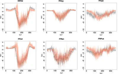
In general, the inclusion of a simplistic SOC routine resulted in a reliable estimation of daily and monthly NEE patterns. While daily and monthly patterns are consistent with EC data, seasonal patterns showed non-negligible misrepresentations, which resulted in negative NSE in most of the cases. This inconsistency may be driven by the strong seasonality in both Reco and GPP [63], which positively affects correlation between EC data and MD results.
NEE patterns during Summer and Fall were much more consistent with measured ones, than Winter and Spring patterns. During these seasons the biases appeared mostly affected by estimation of Reco. The scarcity of the model in representing EBF C fluxes was especially attributable to GPP predictions. 3D-CMCC-PSM and 3D-CMCC FEM inability in predicting GPP in ITCpz and FRPue sites, denoted the necessity to better represent the relations between Mediterranean forests and environmental factors [64; 65]. In FRPue the model well reproduced Spring, Summer and Fall NEE. On the other hand, it showed a bias of around 1gC m-2 d-1 in Winter, suggesting it was missing some particularly importantseasonal processes. For example, evergreen phenology still didn’t consider secondary or continuous growth. Thus, species like Quercus ilex, which exhibit secondary gem sprout in Fall [53], have fresh leaves and mild temperatures to guarantee photosynthetic activity in Fall and Winter, partly explaining 3D-CMCC FEM and 3D-CMCC-PSM systematic underestimation. ITCpz showed the same pattern. However, differently from FRPue, it poorly performed also in early Spring and Summer, especially for GPP patterns. This misbehavior was expected, because of the physical characteristics of the site. In fact, 3D-CMCC FEM soil water dynamics routine was still simplistic, and to date, such other similar models, didn’t include any effect of water table dynamics. On the contrary, ITCpz is characterized with the presence of a shallow groundwater table, which seems to reduce water stress in early Summer [38]. Moreover, we used average daily meteo data collected from the Eddy Covariance stations, and initialized simulations using average structural information found in literature. Uncertainty about those data was potentially high, and could have dramatically affected 3D-CMCC-PSM results.
Summer NEE misrepresentation in DBF was probably affected by the assumption that LAI and photosynthetic capacity reach their maximum in early Summer, alongside. On the contrary, maximum photosynthetic capacity may be reached in late summer, and vary across the canopy. Without taking this into account, GPP could be overestimated up to 40% [66]. Notwithstanding, comparing model outputs with published works [67; 68] these defects are common also for other PBMs.
Seasonal patterns showed that the model consistently misrepresented NEE in Winter, suggesting that Reco still needs to be improved. Especially for DBF sites (e.g. DEHai), Winter Reco was mostly driven by RH. RH was exponentially affected by soil temperatures and especially moisture [69], which are calculated by the model, and could be over-fluctuating in Winter. Moreover, EC data are prone to random noise [70], whose relative impact on performance metrics may be relatively larger.
Figure 8. Patterns in daily NEE (gC m-2 d-1) per DoY (Day of Year) calculated from test-sets on a site level.
Observed EC average patterns (black dotted line) and standard deviation (gray area). Simulated average
patterns (red dotted line) and standard deviation (orange area). First column represents DBF sites, the second
ENF, the third EBF.
It was not always possible to individually validate the different components of respiration. Since EC Reco was not measured but inferred, evaluation metrics should be interpreted as a general ability of 3D-CMCC-PSM in predicting it. Despite daily Reco was noisy, 3D-CMCC-PSM could reproduce respiration processes well enough, at least at monthly timescale.
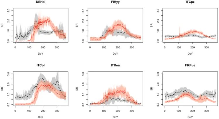
NPP:GPP ranged between 0.37 and 0.62, and was consistent with literature [71; 72; 73]. It was generally higher in DBF (0.49 in DEHai, 0.55 in ITCol), lower in EBF (0.38 in FRPue, 0.41 in ITCpz). These results matched with those of [71] who showed that the ratio between NPP and GPP (CUE) is generally 0.53, ranging from 0.23 to 0.83. CUE was relatively low in FIHyy, where Reco predictions were overestimated: therefore, poor predictability was probably ascribable to excesses in RA.
Figure 9. Patterns in daily Soil Respiration (SR) heterotrophic and autotrophic components (gC m-2 d-1). Patterns
per DoY (Day of Year) calculated from test-sets on a site level. Microbial respiration average patterns (black
dotted line) and standard deviation (gray area). Autotrophic roots respiration average patterns (red dotted line)
and standard deviation (orange area). First column represents DBF sites, the second ENF, the third EBF.
Lack of data to validate the SOC dynamics reduced the spectrum of speculations, which could be statistically analyzed. SOC didn’t change its quantity in ten years; this result was consistent with the theoretical stability of the SOC, an indicator which rarely change within 10 years if no strong disturbance event (e.g. land use change) have occurred [74]. Litter C was highly fluctuating within a year, but its quantity was stable if compared at the end of each year. This suggested that the model realistically represented litter turnover and decomposition, since residues were degraded into humus labile substances about within a year [75]. Microbial Biomass was highly variable, as expected. However, the magnitude of change was too broad throughout the simulations. These results may be related to the use of 5% as the initial active microbial biomass for each site, value that may be far from the equilibrium for different soils. Moreover, tradeoffs within microbial growth and between the environmental conditions may be scarcely represented. As a matter of fact, 3D-CMCC-PSM simulated the soil as having the same physical-chemical structure throughout the profile. This implied that microbes could find the same amount of C, O2, and living space, with no depth limitation.
4.2. 3D-CMCC-PSM uncertainty in estimating NEE
a very reduced amount of species would dominate the different cohorts on landscape to regional scale
According to Figures 6 and 7, and 8 strong uncertainties still reside in timing for the different phenological phases. The biggest source of uncertainty in deciduous stands was driven by the amount of degree days needed to begin vegetative period. The use of a site-specific thermal sum (GDD) to activate vegetation period is widely used, but proven to be very site sensitive, and not very effective for a regional generalization [81]. On the other hand, the processes triggering bud-burst timing are still partly unknown. Moreover, those models proposing a process oriented promoter-inhibition rationale are generally over complex and not prone to spatial generalization [82]. A possible solution in this context is to use remotely sensed data to train a latitudinal explicit regression, constraining GDD estimation.
3D-CMCC-PSM showed high uncertainty also in catching the beginning of the senescence phase. The new phenological scheme didn’t reduce such uncertainty, since it was still using a photoperiod threshold as the senescence phase trigger [38]. Another strong source of uncertainty in Summer GPP may be held by the over simplicity of soil structure and thus of the soil water routine.
As shown in [38], EC data are prone to high uncertainty. We focused on NEE fluxes to reduce the uncertainty cascade related to NEE partitioning. The next natural step will be reframing the model with a hierarchical Bayesian fashion, to quantify error propagation and parameters uncertainty from the posterior distribution [83].
Daily Reco estimation was affected by the cascade of uncertainties related to the calculation of RA and heterotrophic, calculated independently. RA routine may strongly be influenced by uncertainties in RM estimation, which often resulted in RA overestimation. The RM was in fact simulated by a set of empirical relations, which involve: (1) the use of a fixed non-acclimating Q10 factor, whose generality is known to be inaccurate [84]. Moreover, the rationale of Ryan’s RM calculation [85] is affected by uncertainty in estimating daily increment of N pools, generally estimated by forest ecosystem models as a fixed proportion of daily C increment.
5. Conclusions
Soil respiration has a key role in determining NEE in a deterministic fashion [86]. In general, this work showed how the inclusion of a simplistic Soil Carbon routine allowed to predict trends and variability of NEE across the most diffuse European forest ecosystems. Modifications in the phenology scheme produced slight improvements in predicting GPP. However, they were still limited by the correct estimation of bud burst timing, leaf senescence starting point and duration. The use of an optimized parameter-set improved the model’s performance only for those sites where the bio-geophysical processes were correctly reproduced. As a matter of fact, we showed how Mediterranean terrestrial forests, which showed lacks in representing some biological and/or physical processes, performed significantly worse than the other sites, regardless the use of optimized parameters.
In conclusion, we think that 3D-CMCC-PSM reliably estimated NEE and Reco dynamic in a forest ecosystem, especially scaling up daily results to monthly NEE averages. We think that 3D-CMCC-PSM is a solid basis to further explore the effects of soil structure on Carbon and Water dynamics, especially in Mediterranean systems, and be used as a tool for predicting forest growth and ecosystem services, and address questions related to future scenarios forecasting.
Acknowledgements
S.M. was partially supported by the Gordon and Betty Moore Foundation's Data-Driven Discovery Initiative through Grant GBMF4563 to Ethan P. White, and by the GEMINA project to CMCC.
(PON R&C) 2007-2013, through the European Regional Development Fund (ERDF) and national resource (Revolving Fund - Cohesion Action Plan (CAP) MIUR.
This work used eddy covariance data acquired and shared by the FLUXNET community, including these networks: AmeriFlux, AfriFlux, AsiaFlux, CarboAfrica, CarboEuropeIP, CarboItaly, CarboMont, ChinaFlux, Fluxnet-Canada, GreenGrass, ICOS, KoFlux, LBA, NECC, OzFlux-TERN, TCOS-Siberia, and USCCC. The ERA-Interim reanalysis data are provided by ECMWF and processed by LSCE. The FLUXNET eddy covariance data processing and harmonization was carried out by the European Fluxes Database Cluster, AmeriFlux Management Project, and Fluxdata project of FLUXNET, with the support of CDIAC and ICOS Ecosystem Thematic Center, and the OzFlux, ChinaFlux and AsiaFlux offices.
We acknowledge Ethan P. White and Monia Santini for providing critical comments. Carlo Trotta and Giorgio Matteucci for insights about the use of Eddy Covariance data. Sergio Noce for his help in generating GIS based maps.
Author Contributions: S.M. conceived the project, designed the experiments, co-developed the model code, performed the simulations, analyzed the data, and wrote the manuscript. A.C. contributed in designing the experiment, co-developed the model code, and writing the manuscript. T.C. contributed in writing the manuscript. A.N. contributed in writing the manuscript. R.V. contributed in writing the manuscript.
Conflicts of Interest:
The authors declare no conflict of interest.
References
1. Zhang, Y., Li, C., Zhou, X., & Moore, B. (2002). A simulation model linking crop growth and soil biogeochemistry for sustainable agriculture. Ecological Modelling, 151(1), 75-108.
2. Baldocchi, D., Ryu, Y., & Keenan, T. (2016). Terrestrial Carbon Cycle Variability. F1000Research, 5. 3. Göckede M, Foken T, Aubinet M, Aurela M, Banza J, Bernhofer C, et al. 2008, Quality control of
CarboEurope flux data – Part 1: Coupling footprint analyses with flux data quality assessment to evaluate sites in forest ecosystems. Biogeosciences, 5(2):433–50. doi: 10.5194/bg-5-433-2008.
4. Xiao J, Zhuang Q, Law BE, Chen J, Baldocchi DD, Cook DR et al. (2010) A continuous measure of gross primary production for the conterminous U.S. derived from MODIS and AmeriFlux data. Remote Sens Environ 114:576–591 http://dx.doi.org/10.1016/j.rse.2009.10.013.
5. Tang XG, Liu DW, Song KS, Munger JW, Zhang B, Wang ZM (2011) A new model of net ecosystem carbon exchange for the deciduous-dominated forest by integrating MODIS and flux data. Ecol Eng 37:1567–1571 6. Reichstein, M., Falge, E., Baldocchi, D.D., Papale, D., Valentini, R., Aubinet, M., Berbigier, P., Bernhofer, C., Buchmann, N., Gilmanov, T., Granier, A., Gru¨nwald, T., Havra´nkova´, K., Ilvesniemi, H., Janous, D., Knohl, A., Laurela, T., Lohila, A., Loustau, D., Matteucci, G., Meyers, T., Miglietta, F., Ourcival, J.-M., Pumpanen, J., Rambal, S., Rotenberg, E., Sanz, M., Tenhunen, J., Seufert, G., Vaccari, F., Vesala, T., Yakir, D., and Valentini, R. 2005. On the separation of net ecosystem exchange into assimilation and ecosystem respiration: review and improved algorithm. Glob. Change Biol. 11(9): 1–16. doi:10.1111/j.1365-2486. 2005.001002.x.
7. Lasslop, G., Migliavacca, M., Bohrer, G., Reichstein, M., Bahn, M., Ibrom, A., Jacobs, C., Kolari, P., Papale, D., Vesala, T., Wohlfahrt, G., and Cescatti, A. 2012. On the choice of the driving temperature for eddy-covariance carbon dioxide flux partitioning, Biogeosciences, 9, 5243-5259, doi:10.5194/bg-9-5243-2012, 8. Potter, C.S., Randerson, J.T., Field, C.B., Matson, P.A., Vitousek, P.M., Mooney, H.A., Klooster, S.A., 1993.
Terrestrial ecosystem production: a process model based on global satellite and surface data. Global Biogeochem. Cycles 74, 811–841
9. Prince, S.D., Goward, S.N., 1995. Global primary production: a remote sensing approach. J. Biogeogr. 22, 815–835.
10. Mäkelä, A., Landsberg, J., Ek, A.R., Burk, T.E., Ter-Mikaelian, M., et al., 2000. Process-based models for forest ecosystem management: current state of the art and challenges for practical implementation. Tree Physiology 20, 289–298.
12. Yuan, W, Cai, W, Xia, J, Chen, J, Liu, S, Dong, W, Merbold, L, Law, B, Arain, A, Beringer, J, Bernhofer, C, Black, A, Blanken, PD, Cescatti, A, Chen, Y, Francois, L, Gianelle, D, Janssens, IA, Jung, M, Kato, T, Kiely, G, Liu, D, Marcolla, B, Montagnani, L, Raschi, A, Roupsard, O, Varlagin, A & Wohlfahrt, G. 2014. Global comparison of light use efficiency models for simulating terrestrial vegetation gross primary production based on the LaThuile database' Agricultural and Forest Meteorology, vol 192-193, pp. 108-120. DOI: 10.1016/j.agrformet.2014.03.007
13. Cai, W.W., Yuan, W.P., Liang, S.L., Zhang, X.T., Dong, W.J., Xia, J.Z., Fu, Y., Chen, Y., Liu, D., Zhang, Q., 2014. Improved estimations of gross primary production using satellite-derived photosynthetically active radiation. J. Geophys. Res.: Biosci. 119, http://dx.doi.org/10.1002/2013JG002456.
14. Lacointe, A., 2000. Carbon allocation among tree organs. A review of basic processesand representation in functional-structural tree models. Annals of Forest Science57, 521–533.
15. Sievänen R., Nikinmaa E., Nygren P., Ozier-Lafontaine H., Perttunen J., et al. (2000). Components of functional-structural tree models. Annals of Forest Science, Springer Verlag, 57 (5), pp.399-412
16. Lu, M., Nygren, P., Perttunen, J., Pallardy, S.G. & Larsen, D.R. (2011). Application of the functional-structural tree model LIGNUM to growth simulation of short-rotation eastern cottonwood. Silva Fennica 45(3): 431–474
17. Nikinmaa E, Sievänen R, Hölttä T. Dynamics of leaf gas exchange, xylem and phloem transport, water potential and carbohydrate concentration in a realistic 3-D model tree crown. Annals of Botany. 2014;114 653–666.
18. Monteith, J. and Moss, C. J. (1977) Climate and the efficiency of crop production in Britain, Philos. T.R. Soc. Lond., 281, 277–294, doi:10.1098/rstb.1977.0140.
19. Trumbore S. 2006. Carbon respired by terrestrial ecosystems-recent progress and challenges. Global Change Biol., 12 (2006), pp. 141–153
20. Mitchell, S., Beven, K., Freer, J. 2009. Multiple sources of predictive uncertainty in modeled estimates of net ecosystem CO2 exchange, Ecological Modelling, 220, 3259-3270, ISSN 0304-3800, http://dx.doi.org/10.1016/j.ecolmodel.2009.08.021.
21. Yuan, F., Arain, M.A., Barr, A.G., Black, T.A., Bourque, C.P.A., Coursolle, C., Margolis, H.A., Mccaughey, J.H. and Wofsy, S.C. (2008), Modeling analysis of primary controls on net ecosystem productivity of seven boreal and temperate coniferous forests across a continental transect. Global Change Biology, 14: 1765– 1784. doi:10.1111/j.1365-2486.2008.01612.x
22. Xu, B., Y. Yang, P. Li, H. Shen, and J. Fang (2014), Global patterns of ecosystem carbon flux in forests: A biometric databased synthesis, Global Biogeochem. Cycles, 28, 962–973, doi:10.1002/ 2013GB004593. 23. Zobitz, J. M., Moore, D. J. P., Sacks, W. J., Monson, R. K., Bowling, D. R., & Schimel, D. S. (2008). Integration
of process-based soil respiration models with whole-ecosystem CO2 measurements. Ecosystems, 11(2), 250-269. DOI: 10.1007/s10021-007-9120-1
24. Lloyd, J., and Taylor, J.A. 1994. On the temperature dependence of soil respiration. Funct. Ecol. 8(3): 315– 323. doi:10.2307/2389824.
25. Kirschbaum, M.U.F. 2004. Soil respiration under prolonged soil warming: are rate reductions caused by acclimation or substrate loss? Global Change Biology, 10, pp. 1870–1877
26. Xu, J., Chen, J., Brosofske, K., Li, Q., Weintraub, M., Henderson, R., Wilske, B., John, R., Jensen, R., Li, H. et al. 2011. Influence of timber harvesting alternatives on forest soil respiration and its biophysical regulatory factors over a 5-year period in the Missouri Ozarks, Ecosystems, 14, 1310–1327,.
27. Schimel, J. P., and M. N. Weintraub (2003), Soil organic matter does not break itself down the implications of exoenzyme activity on microbial carbon and nitrogen limitation in soil: A theoretical model, Soil Biol. Biochem., 35, 549–563.
28. Tian, H., C. Lu, J. Yang, K. Banger, D. N. Huntzinger, C. R. Schwalm, A. M. Michalak, R. Cook, P. Ciais, D. Hayes, et al. (2015), Global patterns and controls of soil organic carbon dynamics as simulated by multiple terrestrial biosphere models: Current status and future directions, Global Biogeochem. Cycles, 29, 775–792. doi:10.1002/2014GB005021.
29. Chapin III, S., McFarland, J., David McGuire, A., Euskirchen, E. S., Ruess, R. W., & Kielland, K. (2009). The changing global carbon cycle: linking plant–soil carbon dynamics to global consequences. Journal of Ecology, 97(5), 840-850.
31. Knohl, A., Schulze, E. D., Kolle, O., & Buchmann, N. (2003). Large carbon uptake by an unmanaged 250-year-old deciduous forest in Central Germany. Agricultural and Forest Meteorology, 118(3), 151-167. 32. Facelli, José M., and Steward TA Pickett. "Plant litter: its dynamics and effects on plant community
structure." The botanical review 57, no. 1 (1991): 1-32.
33. Richardson AD, Anderson RS, Arain MA et al. (2012) Terrestrial biosphere models need better representation of vegetation phenology: results from the North Ameri- can Carbon Program Site Synthesis. Global Change Biology, 18, 566–584, doi: 10.1111/j.1365-2486.2011.02562.x
34. Kucharik CJ, Barford CC, El Maayar M, Wofsy SC, Monson RK, Baldocchi DD (2006). A multiyear evaluation of a Dynamic Global Vegetation Model at three AmeriFlux forest sites: Vegetation structure, phenology, soil temperature, and CO2 and H2O vapor exchange. Ecological Modelling, 196, 1-31. 35. Ryu SR, Chen J, Noormets A, Bresee MK, Ollinger SV (2008) Comparisons between PnET-Day and eddy
covariance based gross ecosystem production in two Northern Wisconsin forests. Agricultural and Forest Meteorology, 148, 247-256
36. Richardson, Andrew D., Trevor F. Keenan, Mirco Migliavacca, Youngryel Ryu, Oliver Sonnentag, and Michael Toomey. (2013). "Climate change, phenology, and phenological control of vegetation feedbacks to the climate system." Agricultural and Forest Meteorology 169: 156-173.
37. Collalti, A., Perugini, L., Santini, M., Chiti, T., Nolè, A., Matteucci, G., & Valentini, R. (2014). A process-based model to simulate growth in forests with complex structure: Evaluation and use of 3D-CMCC Forest Ecosystem Model in a deciduous forest in Central Italy. Ecological Modelling, 272, 362-378.
38. Collalti, A., Marconi, S., Ibrom, A., Trotta, C., Anav, A., D'andrea, E., ... & Grünwald, T. (2016). Validation of 3D-CMCC Forest Ecosystem Model (v. 5.1) against eddy covariance data for 10 European forest sites. Geoscientific Model Development, 9(2), 479-504.
39. Papale, D., Reichstein, M., Aubinet, M., Canfora, E., Bernhofer, C., Longdoz, B., Kutsch, W., Rambal, S., Valentini, R., Vesala, T., Yakir, D., 2006. Towards a standardized processing of Net Ecosystem Exchange measured with eddy covariance technique: algorithms and uncertainty estimation. Biogeosciences 3, 571– 583.
40. Mencuccini, M., & Bonosi, L. (2001). Leaf/sapwood area ratios in Scots pine show acclimation across Europe. Canadian Journal of Forest Research, 31(3), 442-456.
41. Pilegaard, Kim, Teis N Mikkelsen, Claus Beier, Niels Otto Jensen, Per Ambus, and Helge Ro-poulsen. (2003). “Field Measurements of Atmosphere– Biosphere Interactions in a Danish Beech Forest”, no. December: 315–33.
42. Landsberg J.J., Waring R.H. (1997). A generalised model of forest productivity using simplified concepts of radiation-use efficiency, carbon balance and partitioning. Forest Ecology and Management. vol. 95, p. 209-228.
43. Molina, J. A. E., C. E. Clapp, M. J. Shaffer, F. W. Chichester, and W. E. Larson. (1983). “NCSOIL, A Model of Nitrogen and Carbon Transformations in Soil: Description, Calibration, and Behavior1.” Soil Science Society of America Journal 47 (1): 85. doi:10.2136/sssaj1983.03615995004700010017x.
44. Sollins, P., Homann, P., & Caldwell, B. A. (1996). Stabilization and destabilization of soil organic matter: mechanisms and controls. Geoderma, 74(1-2), 65-105.
45. Fumoto, Tamon, Kazuhiko Kobayashi, Changsheng Li, Kazuyuki Yagi, and Toshihiro Hasegawa. (2008a). “Revising a Process-based Biogeochemistry Model (DNDC) to Simulate Methane Emission from Rice Paddy Fields under Various Residue Management and Fertilizer.” Global Change … 14 (2): 382–402. doi:10.1111/j.1365-2486.2007.01475.x.
46. Coleman, K, and DS Jenkinson. (1999). “ROTHC-26.3.” A Model for the Turnover of Carbon in Soils …, no. November 1999. http://www.uni-kassel.de/~w_dec/Modellierung/wdec-rothc_manual.pdf.
47. Running, Steven W., and E. Raymond Hunt Jr. "Generalization of a forest ecosystem process model for other biomes, BIOME-BCG, and an application for global-scale models." (1993): 141.
48. Keel, Sonja G., and Christina Schädel. (2010) "Expanding leaves of mature deciduous forest trees rapidly become autotrophic." Tree physiology 30, no. 10: 1253-1259.
49. Delpierre, N., E. Dufrêne, K. Soudani, E. Ulrich, S. Cecchini, J. Boé, and C. François. (2009a). “Modelling Interannual and Spatial Variability of Leaf Senescence for Three Deciduous Tree Species in France.” Agricultural and Forest Meteorology 149 (6-7): 938–48. doi:10.1016/j.agrformet.2008.11.014.
51. Chabot, BF, and DJ Hicks. (1982). “The Ecology of Leaf Life Spans.” Annual Review of Ecology and Systematics 13 (1982): 229–59. http://www.jstor.org/stable/2097068
52. Waring, R H, J J Landsberg, and M Williams. (1998). “Net Primary Production of Forests: A Constant Fraction of Gros”, no. 1997.
53. A. Praciak, et al., The CABI encyclopedia of forest trees (CABI, Oxfordshire, UK, 2013).
54. Kuzyakov, Y. (2010). Priming effects: interactions between living and dead organic matter. Soil Biology and Biochemistry, 42(9), 1363-1371.
55. Thornton, P., (2010). Biome BGC version 4.2: Theoretical Framework of Biome-BGC. Technical Documentation.
56. Liang, B., Lehmann, J., Sohi, S. P., Thies, J. E., O’Neill, B., Trujillo, L., ... & Luizão, F. J. (2010). Black carbon affects the cycling of non-black carbon in soil. Organic Geochemistry, 41(2), 206-213.
57. James, G., Witten, D., Hastie, T., & Tibshirani, R. (2013). An introduction to statistical learning (Vol. 6). New York: springer.
58. Walther, B. A., & Moore, J. L. (2005). The concepts of bias, precision and accuracy, and their use in testing the performance of species richness estimators, with a literature review of estimator performance. Ecography, 28(6), 815-829.
59. Keenan, T.F., Ian Baker, Alan Barr, Philippe Ciais, Ken Davis, Michael Dietze, Danillo Dragoni, et al. (2012). “Terrestrial Biosphere Model Performance for Inter-Annual Variability of Land-Atmosphere CO2 Exchange.” Global Change Biology 18 (6): 1971–87. doi:10.1111/j.1365-2486.2012.02678.x.
60. Taylor, K.: Summarizing multiple aspects of model performance in a single diagram, J. Geophys. Res., 106, 7183–7192, 2001.
61. Booth, B. B. B., Jones C. D., Collins, M., Totterdell, I. J., Cox, P. M., Sitch, S., Huntingford, C., Betts, R. A., Harris, G. R., Lloyd, J. (2012), High sensitivity of future global warming to land carbon cycle processes, Environmental Research Letters 7 (2), 024002.
62. Lloyd, J., & Taylor, J. A. (1994). On the temperature dependence of soil respiration. Functional ecology, 315-323.
63. Zhao, Y., Ciais, P., Peylin, P., Viovy, N., Longdoz, B., Bonnefond, J. M., Rambal, S., Klumpp, K., Olioso, A., Cellier, P., Maignan, F., Eglin, T., and Calvet, J. C.: How errors on meteorological variables impact simulated ecosystem fluxes: a case study for six French sites, Biogeosciences, 9, 2537–2564, doi:10.5194/bg-9-2537-2012, 2012.
64. Doblas-Miranda, E., Martínez-Vilalta, J., Lloret, F., Álvarez, A., Ávila, A., Bonet, F. J., ... & Ferrandis, P. (2015). Reassessing global change research priorities in mediterranean terrestrial ecosystems: how far have we come and where do we go from here?. Global Ecology and Biogeography, 24(1), 25-43.
65. Huber-Sanwald, E., Huenneke, L. F., Jackson, R. B., Kinzig, A., Leemans, R., Lodge, D. M., ... & Walker, B. H. (2000). Biodiversity global biodiversity scenarios for the year 2100. Science 287: 17701774Schiffers K, Tielbrger K, Jeltsch F (2010) Changing importance of environmental factors driving secondary succession on molehills. J Veg Sci, 21, 500506Seifan.
66. T Muraoka, H., & Koizumi, H. (2005). Photosynthetic and structural characteristics of canopy and shrub trees in a cool-temperate deciduous broadleaved forest: implication to the ecosystem carbon gain. Agricultural and Forest Meteorology, 134(1), 39-59.
67. Kramer, K, I. Leinonen, H. H. Bartelink, P. Berbigier, M. Borghetti, E. Cienciala, A. J. Dolman, et al. (2002). “Evaluation of Six Process-Based Forest Growth Models Using Eddy-Covariance Measurements of CO 2 and H 2 O Fluxes at Six Forest Sites in Europe”, 213–30.
68. Keenan, T., R. Garcia, S. Sabate, and C. A. Gracia. (2007). “Process Based Forest Modelling: A Thorough Validation And Future Prospects For Mediterranean Forests In A Changing World” 92: 81–92.
69. Zhou, W., Hui, D., & Shen, W. (2014). Effects of soil moisture on the temperature sensitivity of soil heterotrophic respiration: a laboratory incubation study. PloS one, 9(3), e92531.
70. Hollinger, D. Y., & Richardson, A. D. (2005). Uncertainty in eddy covariance measurements and its application to physiological models. Tree physiology, 25(7), 873-885.
71. DeLUCIA, E. V. A. N., Drake, J. E., Thomas, R. B., & GONZALEZ-MELER, M. I. Q. U. E. L. (2007). Forest carbon use efficiency: is respiration a constant fraction of gross primary production?. Global Change Biology, 13(6), 1157-1167.
73. Sabaté, S., Gracia, C. A., & Sánchez, A. (2002). Likely effects of climate change on growth of Quercus ilex, Pinus halepensis, Pinus pinaster, Pinus sylvestris and Fagus sylvatica forests in the Mediterranean region. Forest ecology and management, 162(1), 23-37.
74. Chiti, T., Papale, D., Smith, P., Dalmonech, D., Matteucci, G., Yeluripati, J., ... & Valentini, R. (2010). Predicting changes in soil organic carbon in mediterranean and alpine forests during the Kyoto Protocol commitment periods using the CENTURY model. Soil use and management, 26(4), 475-484.
75. Dickinson, Colin Hedley. 2012. Biology of plant litter decomposition. Vol. 2. Elsevier,
76. Yang, Y., Zhu, Q., Peng, C., Wang, H., Xue, W., Lin, G., ... & Li, S. (2016). A novel approach for modelling vegetation distributions and analysing vegetation sensitivity through trait-climate relationships in China. Scientific reports, 6.
77. Yang, Y., Zhu, Q., Peng, C., Wang, H., & Chen, H. (2015). From plant functional types to plant functional traits: A new paradigm in modelling global vegetation dynamics. Progress in Physical Geography, 39(4), 514-535.
78. Messier, J., McGill, B. J., & Lechowicz, M. J. (2010). How do traits vary across ecological scales? A case for trait-based ecology. Ecology letters, 13(7), 838-848.
79. Claussen, M., L.A. Mysak, A.J. Weaver, M. Crucifix, T. Fichefet, M.-F. Loutre, S.L. Weber, J. Alcamo, V.A. Alexeev, A. Berger, R. Calov, A. Ganopolski, H. Goosse, G. Lohmann, F. Lunkeit, I.I. Mokhov, V. Petoukhov, P. Stone, and Z. Wang, 2002: Earth System Models of Intermediate Complexity: Closing the Gap in the Spectrum of Climate System Models. Climate Dyn., 18, 579-586.
80. Lavorel, S., Díaz, S., Cornelissen, J. H. C., Garnier, E., Harrison, S. P., McIntyre, S., ... & Urcelay, C. (2007). Plant functional types: are we getting any closer to the Holy Grail?. In Terrestrial ecosystems in a changing world (pp. 149-164). Springer Berlin Heidelberg.
81. Schaber, Jörg, and Franz-W Badeck. (2003). “Physiology-Based Phenology Models for Forest Tree Species in Germany.” International Journal of Biometeorology 47 (4): 193–201. doi:10.1007/s00484-003-0171-5. 82. Linkosalo, T., Lappalainen, H. K., & Hari, P. (2008). A comparison of phenological models of leaf bud burst
and flowering of boreal trees using independent observations. Tree Physiol, 28(12), 1873-1882.
83. Uusitalo, L., Lehikoinen, A., Helle, I., & Myrberg, K. (2015). An overview of methods to evaluate uncertainty of deterministic models in decision support. Environmental Modelling & Software, 63, 24-31. 84. Wythers, K. R., Reich, P. B., & Bradford, J. B. (2013). Incorporating temperature-sensitive Q10 and foliar
respiration acclimation algorithms modifies modeled ecosystem responses to global change. Journal of Geophysical Research: Biogeosciences, 118(1), 77-90.
85. Ryan, MG, ST Gower, and RM Hubbard. (1995). “Woody Tissue Maintenance Respiration of Four Conifers in Contrasting Climates.” Oecologia, 133–40.