High power systems for dynamic field control and shielding in the MR environment

(1)

Scholarship@Western

Electronic Thesis and Dissertation Repository

11-18-2011 12:00 AM

High power systems for dynamic field control and shielding in the

MR environment

Dustin W. Haw

The University of Western Ontario Supervisor

Dr. Blaine A. Chronik

The University of Western Ontario Graduate Program in Physics

A thesis submitted in partial fulfillment of the requirements for the degree in Doctor of Philosophy

Follow this and additional works at: https://ir.lib.uwo.ca/etd Part of the Other Physics Commons

Recommended Citation Recommended Citation

Haw, Dustin W., "High power systems for dynamic field control and shielding in the MR environment" (2011). Electronic Thesis and Dissertation Repository. 313.

https://ir.lib.uwo.ca/etd/313

This Dissertation/Thesis is brought to you for free and open access by Scholarship@Western. It has been accepted for inclusion in Electronic Thesis and Dissertation Repository by an authorized administrator of

(2)

(Systems for dynamic field control and shielding in MR) (Thesis format: Integrated Article)

by

Dustin Wesley Haw

Graduate Program in Physics

A thesis submitted in partial fulfillment of the requirements for the degree of

Doctor of Philosophy

The School of Graduate and Postdoctoral Studies The University of Western Ontario

London, Ontario, Canada

(3)

ii

THE UNIVERSITY OF WESTERN ONTARIO School of Graduate and Postdoctoral Studies

CERTIFICATE OF EXAMINATION

Supervisor

______________________________ Dr. Blaine Chronik

Supervisory Committee

______________________________ Dr. Eugene Wong

______________________________ Dr. Martin Zinke-Allman

Examiners

______________________________ Dr. Dennis Parker

______________________________ Dr. Giles Santyr

______________________________ Dr. Neil Gelman

______________________________ Dr. Eugene Wong

The thesis by

Dustin Wesley Haw

entitled:

High power systems for dynamic field control and shielding in the

MR environment

is accepted in partial fulfillment of the requirements for the degree of

Doctor of Philosophy

(4)

iii

Abstract

This thesis addresses several aspects of gradient and shim coil design and fabrication. New

design techniques are coupled with experimental construction methods to expand small

animal insert gradient and shim technology. The design techniques are also applied to other

areas of magnetic resonance hardware.

A custom 2-axis gradient insert coil is designed and fabricated for the purpose of eddy

current characterization. The construction tolerances were examined via bench top

inductance measurements and eddy currents measurement inside a 7.0 T head-only MR

system. A great deal of freedom is available when positioning shielding coils with respect to

their corresponding primary coils in small animal inserts before eddy currents become

prohibitive for imaging.

A new method for actively shielding electromagnets is presented. The minimum

energy method for designing shielding coils of any geometry is developed and validated

against historical methods. Several shielded gradient insert coils are designed, including a

cylindrical gradient set with rectangular shields, which demonstrates the versatility of this

new method. The performance of the shielded insert coils is reported.

A high power custom shim insert coil is designed and optimized for dynamic

shimming applications. This 10-axis shim insert coil is designed to operate at currents higher

than any previously existing shim sets. Several experimental fabrication methods are tested

during the construction of the insert coil. Inductance, resistance and cooling measurements

are conducted and compared to design specifications. Field measurements are taken using a

3-axis field transducer and the shim efficiencies are calculated. Finally mutual inductance

measurements are taken between strongly coupled axes to verify active shielding

performance.

Lastly, the minimum energy method for active shielding is applied to several MR

fringe field type problems. Shields are designed to conform to rooms within an imaging

facility for the purpose of controlling the magnetic footprint of an MR system. The MR

(5)

iv

and a small equipment cabinet located inside the MR room is also fitted with a shield. The

performance of the shields is calculated, and the feasibility of such shields is discussed.

Keywords

magnetic resonance imaging, electromagnetism, electromagnets, magnetic field, gradient

coils, stream function, eddy currents, shim coils, dynamic shimming, inductance, shim

efficiency, active shielding, magnetic susceptibility, homogeneity, minimum energy method,

(6)

v

Co-authorship statement

This thesis contains materials from the following manuscripts:

 Haw D W, Harris C T, Handler W B and Chronik B A 2011. A direct minimum energy method for designing active shields of arbitrary geometry (Submitted to IEEE

Transactions on Magnetics)

This manuscript is reproduced in its entirety and portions thereof in chapter 3. This

manuscript was written by Dustin Haw. All theoretical work, computer modeling,

experiments, data collection, and data analysis was performed by Dustin Haw with the

following exceptions:

Brian Dalrymple and Frank Van Sas provided assistance in machining components for the

insert gradient in chapters 2 and the insert shim set in chapter 4. Martin Klassen wrote the

eddy current measurement pulse sequence, and Joe Gati and Jamu Alford assisted in setting

up the insert gradient on the Varian system in chapter 2. Chad Harris wrote computer code,

performed simulations and coauthored the work in chapter 3. Will handler wrote computer

code for thermal, inductance, and efficiency calculations, as well as a Levenberg-Marquardt

fitting routine. Blaine Chronik, Kyle Gilbert, Timothy Scholl, Will Handler, and Chad Harris

(7)

vi

To my Mom and Dad,

(8)

vii

Acknowledgments

This thesis represents a major commitment from many individuals who contributed their

time, expertise and guidance, both academically and personally.

The completion of this work is largely due to Dr. Blaine Chronik, who supervised me

throughout my graduate career. He provided me with the opportunity and guidance

necessary to make this work a reality, as well as the freedom to explore my own ideas. I am

blessed to have had such a phenomenal role model.

Drs. Will Handler and Tim Scholl have contributed to this project in every way

imaginable from computer programming to final construction. They acted not only as

colleagues, but friends, who made my day to day experience as a grad student more

enjoyable.

Dr. Kyle Gilbert, once a fellow graduate student and now a close friend deserves a

special recognition. His assistance with this work is greatly appreciated, but it‟s his role as a

friend that will never be forgotten.

Brian Dalrymple and Frank Van Sas put a great deal of effort into both the

construction of my insert coils and the development of my shop skills. Without their

expertise this project would be nothing more than a collection of simulations.

I am very grateful for the many people who have worked closely with me during my

degree. They include: James Odegaard, Josh de Bever, Parisa Hudson, Joe Gati, Jamu

Alford, Geron Bindseil and Chad Harris.

Finally, I would like to acknowledge the three people that have had the greatest influence on

(9)

viii

List of tables

Table

1.1 The name and functional form for the most common shim orders ... 17

2.1 Performance data for both shielded gradient axes ... 37

2.2 Eddy current time constants ... 40

3.1 Efficiency and inductance values for the cylindrical gradient set ... 53

3.2 Efficiency and inductance values for the rectangular shield ... 55

4.1 Efficiency, inductance and resistance values for each shim coil ... 74

4.2 Shielding efficiency ratios for zonal shims ... 74

4.3 Simulated and measured mutual inductance for shielded shims ... 76

4.4 Power values for each shim axes ... 78

4.5 Cooling capacity for each cooling layer ... 78

5.1 The specifications for each coil in the 1.0 T main magnet ... 95

5.2 Performance parameters for the MR room shield ... 106

5.3 The performance parameters of both the adjacent room shields ... 110

5.4 Performancevalues for the shielded cabinet ... 117

5.5 Current values for each cabinet shield and field values ... 118

(13)

xii

List of figures

Figure

1.1 Depiction of the magnetization vector ... 3

1.2 A schematic representation of a typical MR system ... 6

1.3 A picture of two gradient coils ... 14

1.4 The magnetic field profile for a spherical piece of iron ... 21

2.1 The primary z-gradient wire pattern ... 30

2.2 Both the z-primary and z-shield ... 31

2.3 The individual quadrants of the y-coil ... 32

2.4 Fully constructed insert coil ... 32

2.5 The geometry of the gradient insert coil ... 33

2.6 Bench measurement setup for insert coil ... 34

2.7 Illustration of the pulse sequence ... 35

2.8 Inductance plots for insert coil ... 38

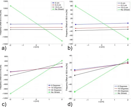
2.9 Frequency measurements at two RF positions ... 39

2.10 Fit frequency data and residual ... 40

2.11 Frequency offsets at each RF position ... 41

3.1 The current density profile along the z-axis ... 53

3.2 The magnetic field profiles for the z-gradient ... 54

3.3 The wire pattern for the planar y-gradient coil ... 55

3.4 The wire patterns for the cylindrical gradient and shields... 56

3.5 The magnetic field profiles for the gradient with rectangular shield ... 57

4.1 Simulated wire pattern for each coil in the shim set ... 73

4.2 Fitted and simulated magnetic field profiles ... 75

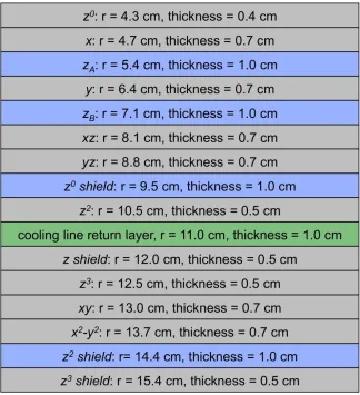
4.3 Schematic representation showing the ordering of the shim layers ... 77

4.4 A photograph of the z0-primary coil ... 79

4.5 A photograph of the zB-layer ... 80

4.6 A photograph of a thumbprint of the xz-shim ... 81

4.7 A photograph of the xz-shim after rolling ... 81

4.8 A photograph of the xz-shim coil being fastened to the insert coil ... 82

4.9 A photograph of the return path layer ... 83

4.10 A photograph of the basic potting procedure for each layer ... 83

5.1 A cut-through schematic representation of the 1.0 T MR system ... 94

5.2 Meshed shielding surface and schematic for MR room shield ... 96

5.3 Meshed surface and schematic for the adjacent room shield ... 98

5.4 Meshed cabinet surface and schematic ... 100

5.5 Wire pattern for the MR room shield ... 103

5.6 Conductor paths on each wall of the room ... 104

5.7 Plot of the magnetic field lines for MR room shield ... 105

(14)

xiii

5.9 Wire pattern of the room adjacent along the x-direction ... 107

5.10 Wire patterns on each of the individual walls of the adjacent room ... 108

5.11 The field lines for the MR system and transverse adjacent room shield ... 109

5.12 The histograms of field magnitudes with transverse shield ... 110

5.13 Wire pattern for the room adjacent to the MR system along the z-direction ... 111

5.14 Wire patterns of each wall for the longitudinally adjacent shielded room ... 112

5.15 Magnetic field lines for the longitudinally adjacent room shield ... 113

5.16 Histograms of field magnitude for longitudinally adjacent room shield ... 114

5.17 Wire pattern for the shielded cabinet ... 114

5.18 Individual wire patterns on each face of the cabinet ... 115

5.19 Magnetic field lines for the MR system and shielded cabinet ... 116

5.20 Magnetic field histograms for shielded cabinet ... 117

5.21 Magnetic field histograms for dynamic cabinet ... 119

5.22 Translational motion field histograms for dynamic cart shield ... 121

(15)

Chapter 1

1 Introduction

1.1 Introduction to magnetic resonance imaging

Magnetic resonance imaging (MRI) is an imaging technique that is renowned for its

ability to generate excellent anatomical images of soft tissues, as well as functional

images of many varieties. MRI measures the changing magnetic flux produced by

non-zero magnetic moments precessing in a magnetic field. Typically it is the protons in fat

and water in the human body of interest, but other nuclei with non-zero magnetic

moments can be imaged as well. The signal acquired in MRI is proportional to the

density of magnetic moments in the sample and is weighted by their phenomenological

relaxation rates, which are tissue or material specific.

The purpose of this introductory chapter is not to provide a complete overview of

MRI, but rather to highlight certain areas that are of particular importance to

understanding the methods and techniques that are presented in this work. This chapter

will discuss the signal acquired in a basic MR experiment from a classical perspective,

focusing on the constituents that are relevant to the work presented in this thesis. The

main hardware components of a typical MR system and their impact on the acquired

signal will be discussed. Finally, several types of magnetic field imperfections and their

effects on the imaging process will be addressed.

The concepts presented in this chapter only represent a small fraction of the MR

basics. For a complete treatment of MRI several textbooks can be consulted (1-4).

1.2 Nuclear magnetic resonance (NMR) and signal

In conventional MRI a sample is placed in a strong, static, and homogenous magnetic

field, with direction along the axis of the MR system (z-axis) and magnitude B0. The

result of the magnetic field is two-fold: a preferential alignment of the magnetic moments

(16)

with a precession about the magnetic field axis at a frequency, , given by the Larmor

equation:

, (1.1)

where γ is the gyromagnetic ratio, which is rad/s/T for protons. The

preference for the moments to align with the field is on the order of a few parts per

million (ppm). However, the presence of Avogadro's number of magnetic moments

results in a net magnetization, , of the sample. When the magnetic moments are in

thermal equilibrium, the magnitude of magnetization generated is well approximated by:

, (1.2)

where is Planck‟s constant divided by 2 is the average thermal energy of the

nuclei in the sample, and is the density of magnetic moments as a function of

sample position.

By applying a time-varying magnetic field at the Larmor frequency and

orthogonal to , the net magnetization can be perturbed and will precess around its

equilibrium position in the transverse plane. This precession results in a changing

magnetic flux that will induce a voltage in a radiofrequency (RF) coil if placed

orthogonal to the main field as depicted in figure 1.1. The induced electromotive force

(EMF) in the RF coil is linearly proportional to the signal acquired in MRI, and is given

by the principle of reciprocity:

. (1.3)

The principle of reciprocity describes the EMF as the summation of magnetization within

(17)

Figure 1.1: Depiction of the magnetization vector as it precesses in the transverse plane after it has been perturbed from equilibrium. The RF coil is placed orthogonal to the plane of precession and can detect the changing magnetic flux from the rotating magnetization.

The net magnetization in the transverse plane decays over time due to dephasing

of the individual magnetic moments, and the original longitudinal magnetization

recovers. Expressions for the longitudinal and transverse components of the

magnetization can be solved for via the Bloch equation (5):

_(1.4)

_{. (1.5)}

is the magnetization in the transverse plane. is the phenomenological time

constant that describes the rate at which longitudinal magnetization regrowth occurs.

is tissue/material specific and varies with position in the sample. can then be

given by:

, (1.6)

where is the phenomenological time constant that describes the decay of transverse

(18)

the sample. is the contribution to from all other sources of magnetic field.

These include things like B0 inhomogeneity, field variations due to differences in

magnetic susceptibility, and diffusion just to name a few. If all the longitudinal

magnetization is tipped into the transverse plane then: . The x- and

y-components of the net magnetization vector are given by:

(1.7)

. (1.8)

In order to spatially encode the signal generated in MRI, a magnetic field gradient

is applied across the sample. When this gradient, , is applied, the transverse

magnetization accrues extra phase depending on its position in the gradient field. This

accrued phase is given by:

. (1.9)

The applied gradient field makes the phase and precession frequency of the

magnetization a function of position in the sample – this spatial dependence is what

allows images to be created. When we consider the extra phase accrued from the

magnetic field gradients the expression for the net magnetization vector becomes:

_{. (1.10)}

By substituting the expressions for the longitudinal and transverse magnetization

into the reciprocity relation (equation 1.3) the EMF induced in the detection coil can be

solved for:

_(1.11)

Equation 1.11 can be simplified by taking the time derivative and accounting for the large

(19)

1/T1 is on the order of 100 - 101 Hz, 1/ is on the order of 101 - 102 Hz, and

is on the order of 105 - 106 Hz. is approximately 107-108 Hz and dominates the

other terms, meaning they can be neglected. The result is:

_{. (1.12)}

Equation 1.12 can be further simplified by expressing the individual components of the

RF magnetic field in terms of their magnitude and angle:

(1.13)

. (1.14)

The EMF is then given by:

. (1.15)

If a complex MR signal is defined such that: , then the acquired

MR signal is given by the relation:

. (1.16)

This expression does not explicitly consider every aspect of the MR signal; other factors

can influence the MR signal. However, the factors considered are the most important for

the work that will follow. Of particular importance are the effects associated with the

term , which will be discussed many times throughout this thesis.

1.3 MRI hardware

A typical MR system consists of four major hardware subsystems: the main magnet,

radiofrequency coils, gradient coils and shim coils, as depicted in figure 1.2. Each

(20)

equation derived above (equation 1.16). This section provides a discussion of each

hardware component and highlights its effect on the signal equation. In the case of

gradient and shim coils a more thorough outline will be given as necessary background

for this work.

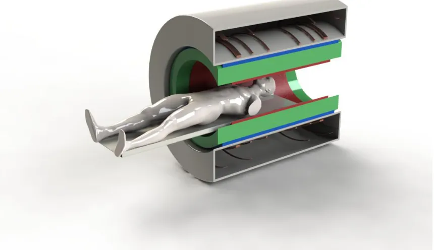
Figure 1.2: A schematic representation of a typical MR system. Part of the system is cut away so the various hardware components are visible. The brown bundles inside the gray casing are the superconducting main magnet wire. The shim coils are shown in blue, the gradients in green and the RF coil is represented by the red cylinder. Image courtesy Will Handler.

1.3.1 Main magnets

The primary function of the main magnet in an MR scanner is to force a population of

magnetic moments to align with the main magnetic field, resulting in a net magnetization

of the sample. Because MRI is a very low signal-to-noise (SNR) phenomenon the field

produced by the main magnet needs to be very strong, but also time independent and

(21)

superconducting material, almost always niobium-titanium (Nb-Ti), which can support a

high amount of current with negligible resistance. Nb-Ti has a critical superconducting

temperature of 10 K, which means it must be continuously cooled in order to remain

superconducting. To remain at the critical temperature the superconducting wires are

typically immersed in liquid helium, which has a boiling point of 4.2 K. Research

scanners have been produced using resistive and permanent magnet technology (6), but

superconducting systems remain dominant in the clinical setting.

The ultimate effect that the main magnetic field has on the signal acquired in a

MR experiment comes from two separate parts of the imaging process. First, the amount

of bulk magnetization present in a sample, as given by equation 1.2, is linearly

proportional to B0. Second, during the acquisition stage the EMF is dependent on the

time derivative of the magnetization vector, given by equation 1.3, which makes the

signal proportional to the Larmor frequency as well. Provided B0 is responsible for both

the polarization of the sample and is present during the acquisition of signal, the resulting

dependency on the main field is B02. This dependence on field strength is responsible for

the continual trend towards higher field strengths in MRI.

Magnetic field strengths for clinical whole-body systems range from about 0.5 –

3.0 T at present. However, research systems are available up to 7.0 T above. Small

animal scanners routinely operate at higher fields, and NMR spectrometers are available

at field strengths even higher yet. For clinical MRI current regulations prohibit the use of

field strengths over 3.0 T (7).

In addition to being strong, the main field must also be extremely homogeneous.

The homogeneity requirement comes from the (r,t) dependence in the signal equation.

The inhomogeneities of the main field must be sufficiently small so they do not dominate

the applied gradient (Gapplied>>Ginhomo). This places a stringent requirement on main field

uniformity. At present modern scanners have main magnetic fields that can be

homogenous to 1 ppm over 50.0 cm imaging volumes with the help of superconducting

and ferromagnetic shims, which will be discussed later. In addition to the spatial

(22)

Superconducting magnets produce fields that can vary less than a T/hour; a field

varying less than a few ppm over the total imaging time would be considered time

independent for most MR applications, thus superconducting fields are sufficiently stable

for MRI. That is not the case for systems using resistive technology (8).

Aside from the critical properties discussed, other desirable characteristics that

must be considered in the design of a main magnet consist of: patient access and comfort,

cost of the magnet, fringe field minimization, weight and size.

1.3.2 RF coils

Radiofrequency (RF) coils are responsible for both the excitation and acquisition of the

MR signal. Looking back at the signal equation it can be seen that the signal received is

weighted by the sensitivity profile of the RF coil (B1(r)). This means that RF field

profiles need to be uniform to avoid intensity shading in images, and that more sensitive

coils will give larger signals. RF coils are tuned to resonate at the Larmor frequency of

the nuclei that is being imaged, which is 63.87 MHz at 1.5 T and 127.7 MHz at 3.0 T for

protons.

A single coil can be used to excite the magnetization (transmit) and detect

(receive), however, it is also possible to use separate coils. Because desirable

characteristics differ for transmission and reception, often two separate coils are used.

The driving quality behind transmit RF coils is the need to generate a

homogeneous excitation across the sample. Many types and geometries of transmit coils

exist, but because of the homogeneity requirement transmit coils tend to be larger volume

coils as compared to receive coils. A very common geometric design for transmit coils is

the birdcage coil (9). However, the trend towards higher field MR systems has caused

RF engineers to rethink the traditional transmit RF coils (10).

A second consideration in designing an RF transmit coil is the time it takes for the

RF coil to tip the magnetization vector into the transverse plane. The angle at which the

(23)



B₁_rf. (1.17)

So the stronger the B1 field the less time required for a given flip angle, which is

important because time is always paramount in MRI.

Another extremely important aspect of RF transmit coils is power deposition.

When transmit fields perturb the magnetization from thermal equilibrium, energy is

deposited in the sample as heat via a Faraday induction effect. Guidelines and

regulations have been established that dictate acceptable limits on specific absorption

rates (SAR) of radiation deposited in the body (7,11). Limiting local SAR values in the

human body to approximately 8 W/kg, ensures no significant temperature increase will

occur. At 1.5 T the RF wavelengths are long enough that SAR deposition is relatively

uniform, but as field strength increases, wavelength decreases, and local hot spots

become a major concern.

The two major factors that drive RF receive coil design are the sensitivity profile

and noise characteristics of the coil. RF receive coils can take on many geometrical

forms as a result of trying to optimize for both of these considerations (12). The

sensitivity profile of a receive coil is heavily dependent on its geometry. In particular it

is extremely important to get the RF coil as close to the sample as possible. This

requirement is evident in a clinical setting, where RF coils have been customized to

enclose almost every part of the human body.

The noise in an RF receive coil results from the intrinsic noise in the RF coil

itself, and the coupling between the RF coil and the sample (as well as radiation coupling

in principle). When sample noise is a dominant factor, reducing the volume of the

sample that the coil is sensitive over will reduce the noise. The trade off is that the field

of view of the RF coil is reduced – a problem solved by using multiple receive coils.

Phased array RF coils are sets of coils that can have their signals combined to be

sensitive over a volume larger than that of any of the individual coils. Smaller coils have

better SNR because they have small noise volumes. So it can be beneficial to combine

(24)

coil. For array coils to benefit from the noise reduction associated with smaller coils, the

noise of each individual RF coil must be uncorrelated with the others. Parallel imaging

techniques that greatly reduce the acquisition times for many types of MR sequences are

largely made possible by phased array RF coils (13,14). Phased array coils are also

showing promise in dealing with the problems of transmission field homogeneity in

higher field MR (15).

1.3.3 Gradient coils and shim coils

For ease of explanation and to stay with conventional thought, gradient coils and shim

coils will be discussed as separate entities. However, the idea that these sets of coils

should, and in the future, hopefully will be thought of as a single set of coils responsible

for “dynamic field control” during the imaging process is briefly discussed.

Traditionally in MRI gradient coils and shim coils have been thought of as

separate hardware subsystems, each playing a different role in the imaging process.

Although each set of coils does in fact play a different role in terms of functionality, they

both accomplish the same task, which is to control the magnetic field during the imaging

process. To further strengthen the argument that gradient and shim coils should and can

be viewed as a single entity, it is noted that each coil is just an individual term in a

harmonic expansion of the magnetic field and that gradients play a direct role in the

shimming process as the linear shims. Lastly, both types of coils leave their mark on the

same term ( ) in the MR signal equation. For this work it is instructive to think of

the gradients as being a special subset of the shim coils that provide the image encoding

fields.

1.3.3.1 Gradient coils

The primary responsibility of the gradient coils is to spatially encode the position of the

magnetic moments in a sample. They accomplish this task via a linearly varying

magnetic field across the sample, which makes the precession frequency, or phase, of the

nuclei at each position different. This allows differentiation between locations in the

(25)

each Cartesian axis, that produce a magnetic field such that its z-component varies

linearly along the direction that defines that coil:

(1.18 a)

(1.18 b)

. (1.18 c)

Gxis the x-gradient, Gy is the y-gradient and Gz is the z-gradient. The Gxand Gy gradients

are commonly referred to as transverse gradients and the Gz gradient is known as the

longitudinal gradient.

There are numerous properties associated with gradient coils that determine their

effectiveness. Among the most important design characteristics are: gradient efficiency,

switching speed, gradient uniformity, inductance, and power deposition. Efficiency,

uniformity, inductance and resistance are properties of the gradient coil itself, while

gradient strength, slew-rate, and power deposition are properties of both the gradient coil

and its amplifier together. The gradient strength, measured in mT/m or G/cm, is

important because it dictates the resolution that can be achieved for a given imaging time.

The switching speed, or slew rate, is measured in mT/m/ms and tells how fast a gradient

coil can be turned on and off. Fast imaging applications require gradients that can be

switched very quickly (greater than 1.0 kHz). Gradient uniformity is the size of volume

over which the gradient field is sufficiently uniform for imaging, and is a major

consideration in gradient coil design as it dictates the physical size of the coil, a property

that influences almost all other coil characteristics. The inductance and power of a

gradient coil are important as they must be considered when selecting an amplifier. In

addition to amplifier matching, the power dissipated in a gradient also effects the duty

cycle that can be achieved and the need, or lack thereof, for external cooling.

Other aspects that are important to the design of a gradient coil might include:

forces and torques on the coil, acoustic noise and patient access. Switching the gradient

(26)

individual wires themselves and could result in large net forces or torques on the entire

structure if one is not careful. This rapid switching also results in significant acoustic

noise as the switching frequencies are usually in the audible range.

Evaluating the overall performance of a gradient coil can be a difficult task given

that there is a tradeoff between many of the performance metrics for gradients coils. Two

quantities that are relevant in quantifying practical gradient performance are: gradient

strength and switching speed. These quantities are dependent on not only the gradient

coil, but also the amplifier, and are given by:

(1.19)

, (1.20)

where  is the gradient efficiency in mT/m/A, I is the current in the coil, V is the voltage

applied, and L is the inductance of the coil. Comparing different gradient coils via

equations 1.19 and 1.20 poses a problem in that the gradient efficiency and inductance of

the coil are heavily dependent on the size of the imaging region, size of the coil, and most

importantly the number of windings used. One solution is to use figure of merit metrics

(16):

(1.21)

, (1.22)

where r is the radius of the coil, L is the coil inductance, and R is the coil resistance. ML

is known as the inductive merit and MR is known as the resistive merit and these values

are independent of coil size making them acceptable for direct comparison.

Another important aspect of gradient coils is the concomitant magnetic fields that

are produced along with the desired linear field variation. The linear field variation that

(27)

without accompaniment of other fields. As an example consider a linearly varying field

along x (x-gradient):

. (1.23)

If no sources are present then: , but: , so it can be seen that

another field component must be present to satisfy Maxwell‟s equations. These

concomitant magnetic fields can result in image artefacts if sufficiently large, although at

higher field MR (1.5 T and up) they are not a major concern.

It was noted in the discussion of radiofrequency coils that the performance of

such coils was ultimately limited by the amount of energy deposited in the body.

Gradient coils do not cause heating in body tissue because they operate at lower

frequencies than RF coils, which means they have lower dB/dt values. However, another

physiological effect limits the full use of their capabilities – peripheral nerve stimulation

(17). Peripheral nerve stimulation occurs because the gradient coils are switched on and

off rapidly, resulting in time varying magnetic fields that happen to be at the right

frequency for reaction with the peripheral nervous system of humans.

For this work a brief look at the history of gradient design and the current state of

gradient technology is warranted. Initial gradient design methods were crude yet robust

in that they produced coils that were sufficient enough to survive for a significant period

of time. The two classic examples of these early “building block” gradient coils are the

common Maxwell pair (18) (longitudinal gradient) and the Golay coil (19) (transverse

gradient). Both these designs are achieved by expanding the magnetic field generated

from an arch of wire and solving for the positions of the arch, such that the only field

term left is the one desired. These early types of gradient coils were less efficient and not

capable of the switching speeds of today‟s gradient coils. It was not until the 1980‟s that

the need for faster and stronger gradients was even apparent (20). New imaging

techniques began to place higher demands on gradient technology and the result was

distributed winding gradient coils. Distributed winding coils are better approximations to

continuous current densities than previous coils. A visual comparison of distributed

(28)

(29)

Many design methods exist for distributed winding gradient coils: matrix

inversion methods (21), stream function methods (22), and target field methods (23), but

the basic idea is the same for all. The desired magnetic field profile is parameterized in

terms of the current density on a coil former (usually a cylinder), and then that current

density is solved for. An approximation method is then used to determine where to place

wires to best represent that continuous current density. Many of these methods have the

ability to optimize gradient designs with respect to particular parameters, such as power

or inductance (24,25). The technique for this is to parameterize not just the magnetic

field but the desired characteristic in terms of current density and minimize an error

function that contains both. Modern gradient design techniques have now pushed past

the restriction to simple geometries using Boundary Element (BE) methods (26,27,28)

and the ability to create gradient coils on any arbitrary geometry is now possible.

Today‟s state of the art clinical whole body gradient coils are capable of 50.0 mT/m and

slew rates of several hundred mT/m/ms. Research gradients are available that routinely

reach much higher gradient strengths and much faster slew rates, although over smaller

imaging volumes, making them not directly comparable (29).

1.3.3.2 Shim coils

As was mentioned above, the shim coils in an MR system influence the term in

the signal equation, just like the gradients. However, the goal of the shim coils is not to

create a frequency or phase dispersion across the sample, but to correct for the one that

exists from sources other than the gradients.

Shim coils accomplish this correction by producing specific magnetic field

variations that attempt to cancel out the field variations that arise from B0 inhomogeneity,

and other sources, which will be discussed in further detail below. There are typically

two sub-categories of shim coils in a conventional MR scanner. The first category is

passive shim coils. Passive shim coils are responsible for correcting (shimming) the field

distortions that result from imperfections in the system and the magnetic environment

around the system. There are often two sets of passive shims: a set of superconducting

wire wound shim coils housed inside the cryostat with the main magnet windings, and a

(30)

typically trays of iron discs that are strategically placed to correct for field distortions.

Both the superconducting and ferromagnetic passive shims are optimized when the

magnet is installed, and are rarely adjusted afterwards.

The second category of shim coils, and the one of greatest importance to this

work, is room temperature resistive shims. Just like the gradient coil set, these shim sets

consist of resistive wire wound electromagnets grouped together inside the bore of the

scanner. What makes these different from passive shims is that the current can be

adjusted to change the field variation that the shim set creates. Room temperature shims

must correct for field distortions that are sample specific (more on sample specific

distortions later), which means they must be adjustable and capable of generating a

variety of different field variations.

The most common method for generating a shim set that is capable of correcting a

wide variety of fields is to make individual coils that approximate orthogonal field

variations over the volume of interest and use those coils in linear combinations with

each to approximate the necessary shim field. Because there is no current flowing in the

imaging region over which shimming is to occur, the coils of interest are ones that satisfy

Laplace‟s equation. It has been described by Roméo and Hoult (30) that the shim field

can be characterized by spherical harmonics which are solutions to Laplace‟s equation:

, (1.24)

where are the associated Legendre polynomials. The desired field variation for each

shim coil is given by the corresponding harmonic term, and solving for the current

necessary on a coil former is accomplished via any of the methods previously discussed

for gradients. Modern shim sets typically consist of all zero, first and second order

spherical harmonics, and often third order coils are added for further corrective power.

The more orders that are added the greater the shimming ability, but bore space and the

Biot-Savart law ultimately place constraints on how many shims can effectively be

added. Table 1.1 gives the name and functional form of spherical harmonic shims up to

(31)

Table 1.1: The name and functional form for the most common shim orders. l and m are given by equation 1.24.

l m Shim Name Functional Form

1 0 z z

1 1 x x

1 -1 y y

2 0 z2 z2-(x2+y2)/2

2 1 zx zx

2 -1 zy zy

2 2 x2-y2 x2-y2

2 -2 xy 2xy

3 0 z3 z3-3z(x2+y2)/2

3 1 z2x z2x-x(x2+y2)/4

3 -1 z2y z2y-y(x2+y2)/4

3 2 z(x2-y2) z(x2-y2)

3 -2 zxy zxy

3 3 x3 x3-3xy2

3 -3 y3 3x2y-y3

Other unconventional shim systems exist outside the standard spherical harmonic

room temperature shim set that deserve some attention. One such method uses

ferromagnetic material to shim sample specific field distortions (31). Because certain

parts of the human anatomy are frequently imaged, it is possible to create an array of

ferromagnetic material that accurately shims part of the human body, provided that the

field distortions from person to person are similar enough. A second type of

unconventional shim set makes use of many circular loops, like an RF array, to construct

the necessary shim fields (32). This method is inherently low power, and gives the

ability to produce higher order harmonic terms that aren‟t generally available in a

traditional shim set. Furthermore, it has the ability to produce field variations that are not

approximated by a sum of low order spherical harmonics. This method attempts to

overcome the limitations placed on shim sets by the bore and Biot-Savart law. Another

technique for overcoming these constraints is introduced in chapter 4 of this work.

1.4 Magnetic field imperfections

Throughout this chapter the major imaging fields in MR have been discussed (the static

(32)

magnetic fields are not perfect in reality has been introduced through the concepts of

homogeneity and the need for shim coils. Magnetic field imperfections are very common

in MR. They result from many different sources and can affect any one of the fields

necessary for imaging. In this section several sources of magnetic field imperfections

will be discussed: system and sample related B0 inhomogeneities, and eddy currents.

As has been the theme so far, field imperfections impact the term in the

signal equation. It was mentioned previously that there is a phase dispersion across the

sample that is related to the applied gradient field. However, if field imperfections exist

then the phase across the sample is not just a result of the applied gradient ( ), but

also any inhomogeneities ( ). If these effects are accounted for, the phase accrued is

actually:

. (1.25)

The first type of magnetic field distortions are those that arise from imperfections

in the system and its immediate environment. These kinds of imperfections are usually

quite static in nature, although not always. What separates them from others is that they

are corrected for when the MR system is installed and do not require constant attention.

These field distortions may occur because the windings inside an MR system may not be

positioned perfectly. No matter how careful the manufacturing process, windings cannot

be exact, and even so, they can experience considerable electromagnetic and gravitational

forces, which often results in settling over time. Inhomogeneities can also arise from the

surroundings of an MR system. Steel beams in the walls or support structures of the

building can become magnetized and degrade the imaging field. Ferromagnetic material

placed near the scanner for the purpose of shielding can give rise to field distortions.

There can be many field distortions associated with the MR environment, but if they are

static then they can be corrected for during installation, just like the system

imperfections.

A second category of field distortions results from the samples themselves, and

(33)

sample basis. For most materials the magnetization is sustained by the field and is

proportional to it (paramagnetic and diamagnetic). These materials are called linear

media and the induction field, the auxiliary field, and the magnetization are related via

the following equations (33):

(1.26)

, (1.27)

where  is the magnetic permeability, and  is the magnetic susceptibility of the material.

For paramagnetic material:  > 0, and for diamagnetic material: < 0. Biological tissue

has a magnetic susceptibility of approximately -9.2 ppm and air has a magnetic

susceptibility of approximately 0.3 ppm, which can result in small but significant field

distortions at air-tissue boundaries. The magnetic permeability and magnetic

susceptibility are related by:

. (1.28)

Using equations 1.26 – 1.28 the magnetic field can be expressed as:

. (1.29)

So it can be seen that the magnetic field can vary across different material and the

discontinuities at boundaries can give rise to field distortions.

As a practical example consider a spherical piece of material with a magnetic

susceptibility that is different from its surroundings placed in a magnetic field: .

The magnetic field outside can be approximated as a constant term plus a dipole field:

, (1.30)

Where the magnetic dipole moment of the sphere is calculated as:

(34)

The field inside is given by equation 1.29:

. (1.32)

To obtain a solution for boundary conditions must be considered. First the normal

component of B and the tangential components of H must be continuous across the

spherical surface, also very far from the sphere the field must be B0. Given these

conditions:

. (1.33)

Combining equations 1.31-1.33 the solutions for the fields outside and inside the

magnetic sphere are:

(1.34)

. (1.35)

Using equations 1.34 and 1.35 the phase shift that results from the magnetic field

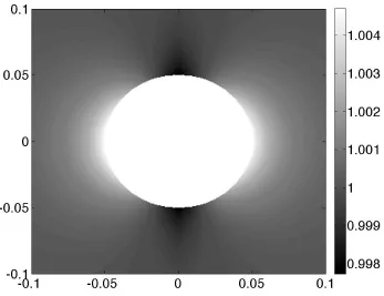
difference can be calculated, making simple models such as this quite useful. Figure 1.4

shows the magnetic field profile for a spherical piece of stainless steel placed in a 1.0 T

uniform field.

Sample induced inhomogeneities are the dominant source of field distortions in

MRI. They can be very difficult to deal with because they are different for every sample.

These inhomogeneities range widely in size, and can be quite severe in places like the

sinus cavity. More exotic situations, such as metallic medical implants, can be so severe

(35)

Figure 1.4: The magnetic field profile on a plane cut through the center of a spherical piece of stainless steel (10.0 cm diameter) placed in a 1.0 T uniform field.

The last type of field error this chapter will address is that of eddy currents. Eddy

currents are not usually mentioned alongside B0 inhomogeneities, but they are magnetic

field imperfections nonetheless.

The dominant cause of eddy currents in MR is the rapidly switching gradient

fields. The MR system itself is constructed of many conducting materials, some of which

are held at very low temperatures inside or in close proximity to the cryostat. These

conductors have the ability to house eddy currents if exposed to large time varying

magnetic fields, which is common to MRI in the form of gradient fields. The mechanism

for eddy current induction is a two step process. First time-varying magnetic fields give

rise to induced electric fields via Faraday‟s Law:

(36)

Then, if a conductor is present, the induced electric fields result in a force on the

electrons:

, (1.37)

which gives rise to eddy currents.

Because of the symmetry of the MR system the eddy fields generally mirror the

pulsed gradient fields that caused them, resulting in less efficient gradients. However,

this is not always the case (35). Time scales for eddy currents in MR vary widely from a

few milliseconds to well over a second for eddy currents that exist in the coldest

structures of the MR system (36). These long time-constant eddy currents are extremely

problematic for imaging, as settling is often required before imaging can continue. The

magnitude of an eddy current is heavily dependent on the system in question,

particularly, the distance between the switching coil and the conducting structures.

There are two standard and widely employed methods for dealing with eddy

currents generated via the gradient coil – pre-emphasis and shielding. Pre-emphasis is a

technique that alters the current waveform sent to the gradient coil, such that the gradient

pulse plus the eddy current it generates will give the desired gradient waveform.

Shielding the gradient coils is also a common method. Almost all whole-body gradient

sets today are actively shielded, which involves placing a second coil between the initial

gradient coil and the rest of the MR system so the field from the initial gradient will be

cancelled at, and beyond, the radius of the shielding coil. This is a technique that will be

discussed heavily throughout this work.

1.5 Thesis overview

This thesis describes advancements made in the design and development of insert

gradient and shim technology. The same design principles applied to insert coils have

also been extended and applied to the fringe field problem posed by MRI.

Chapter 2 examines the size and timing associated with eddy currents generated

(37)

built specifically to measure the construction tolerances associated with shield placement.

Eddy current measurements were conducted in a 7.0 T head only Varian scanner as a

function of the relative shield position with respect to the primary coils. Several unique

eddy currents were isolated and reported.

Chapter 3 outlines a new design tool that allows for shielding coils to be optimized

over any arbitrary geometry without the constraints of previous methods. This new

design method is compared to previous techniques for validation and then applied to a

more exotic situation that extends beyond the capabilities of older analytical methods. A

version of this chapter has been submitted to IEEE Transactions on Magnetic for

publication.

In chapter 4 a shim set is designed for the purpose of dynamic shimming, a

technique that requires shim currents to be updated during an acquisition. This high

power customized shim set is designed, fabricated and bench tested. Performance and

field measurements are reported and the technical challenges associated with designing

and building such an insert shim set are discussed.

In chapter 5 the minimum energy shielding method presented in chapter 3 is

extended and applied to several shielding applications involving the fringe field of an MR

system. Large room-size active shields are designed to limit the extent of the magnetic

field from a 1.0 T MR system. A smaller cabinet-sized shield is designed for the purpose

of protecting non-MR compatible equipment. Lastly, two smaller multi-layer shields are

designed to react dynamically to motion relative to the MR system. The performance of

the shields are reported and the practical feasibility is discussed.

Finally chapter 6 discusses the conclusions that can be drawn from the work

presented. Work that has yet to be completed along with interesting future directions for

(38)

1.6 References

1. Haacke EM, Brown RW, Thompson MR, Venkatesan R. Magnetic Resonance Imaging: Principles and Sequence Design. New York: John Wiley & Sons Inc.; 1999.

2. Bernstein MA, King KF, Zhou XJ. Handbook of MRI Pulse Sequences. Burlington: Elsevier Academic Press; 2004.

3. Cowan B. Nuclear Magnetic Resonance and Relaxation. Cambridge: Cambridge University Press; 1997.

4. Levitt MH. Spin Dynamics: Basics of Nuclear Magnetic Resonance. West Sussex: John Wiley & Sons Ltd.; 2001.

5. Bloch F. 1946 Nuclear Induction. Physical Review;70(7-8):460-474.

6. Gilbert KM, Handler WB, Scholl TJ, Odegaard JW, Chronik BA. 2006 Design of field-cycled magnetic resonance systems for small animal imaging. Physics in Medicine and Biology;51(11):2825-2841.

7. Zaremba LA. FDA Guidelines for Magnetic Resonance Equipment Safety. In: Administration FaD, editor. Center for Devices and Radiological Health; 2011.

8. Gilbert KM, Scholl TJ, Handler WB, Alford JK, Chronik BA. 2009 Evaluation of a Positron Emission Tomography (PET)-Compatible Field-Cycled MRI (FCMRI) Scanner. Magnetic Resonance in Medicine;62(4):1017-1025.

9. Hayes CE, Edelstein WA, Schenck JF, Mueller OM, Eash M. 1985 An Efficient, Highly Homogeneous Radiofrequency Coil for Whole-Body Nmr Imaging at 1.5-T. Journal of Magnetic Resonance;63(3):622-628.

10. Ibrahim TS, Lee R, Baertlein BA, Abduljalil AM, Zhu H, Robitaille PML. 2001 Effect of RF coil excitation on field inhomogeneity at ultra high fields: A field optimized TEM resonator. Magnetic Resonance Imaging;19(10):1339-1347.

11. Collins CM, Li SZ, Smith MB. 1998 SAR and B-1 field distributions in a heterogeneous human head model within a birdcage coil. Magnetic Resonance in Medicine;40(6):847-856.

(39)

13. Sodickson DK, Manning WJ. 1997 Simultaneous acquisition of spatial harmonics (SMASH): Fast imaging with radiofrequency coil arrays. Magnetic Resonance in Medicine;38(4):591-603.

14. Boesiger P, Pruessmann KP, Weiger M, Scheidegger MB. 1999 SENSE: Sensitivity encoding for fast MRI. Magnetic Resonance in Medicine;42(5):952-962.

15. Katscher U, Bornert P, Leussler C, van den Brink JS. 2003 Transmit SENSE. Magnetic Resonance in Medicine;49(1):144-150.

16. Turner R. 1993 Gradient Coil Design - a Review of Methods. Magnetic Resonance Imaging;11(7):903-920.

17. Chronik BA, Rutt BK. 2001 Simple linear formulation for magnetostimulation specific to MRI gradient coils. Magnetic Resonance in Medicine;45(5):916-919.

18. Bangert V, Mansfield P. 1982 Magnetic-Field Gradient Coils for Nmr Imaging. Journal of Physics E-Scientific Instruments;15(2):235-239.

19. Golay M; Magnetic field control apparatus. US patent 3,515,979. 1957 November 4.

20. Suits BH, Wilken DE. 1989 Improving Magnetic-Field Gradient Coils for Nmr Imaging. Journal of Physics E-Scientific Instruments;22(8):565-573.

21. Wong EC, Jesmanowicz A, Hyde JS. 1991 Coil Optimization for Mri by Conjugate-Gradient Descent. Magnetic Resonance in Medicine;21(1):39-48.

22. Edelstein W, Schenck J; A stream function method for coil construction. U.S. 1987.

23. Turner R. 1986 A Target Field Approach to Optimal Coil Design. Journal of Physics D-Applied Physics;19(8):L147-L151.

24. Carlson JW, Derby KA, Hawryszko KC, Weideman M. 1992 Design and Evaluation of Shielded Gradient Coils. Magnetic Resonance in Medicine;26(2):191-206.

25. Turner R. 1988 Minimum Inductance Coils. Journal of Physics E-Scientific

Instruments;21(10):948-952.

(40)

27. Lemdiasov RA, Ludwig R. 2005 A stream function method for gradient coil design. Concepts in Magnetic Resonance Part B-Magnetic Resonance Engineering;26B(1):67-80.

28. Poole M, Bowtell R. 2007 Novel gradient coils designed using a boundary element method. Concepts in Magnetic Resonance Part B-Magnetic Resonance Engineering;31B(3):162-175.

29. Chronik BA, Alejski A, Rutt BK. 2000 Design and fabrication of a three-axis edge ROU head and neck gradient coil. Magnetic Resonance in Medicine;44(6):955-963.

30. Romeo F, Hoult DI. 1984 Magnet Field Profiling - Analysis and Correcting Coil Design. Magnetic Resonance in Medicine;1(1):44-65.

31. Juchem C, Muller-Bierl B, Schick F, Logothetis NK, Pfeuffer J. 2006 Combined passive and active shimming for in vivo MR spectroscopy at high magnetic fields. Journal of Magnetic Resonance;183(2):278-289.

32. Juchem C, Nixon TW, McIntyre S, Rothman DL, de Graaf RA. 2010 Magnetic field modeling with a set of individual localized coils. Journal of Magnetic Resonance;204(2):281-289.

33. Jackson JD. Classical Electrodynamics. New York: John Wiley & Sons Inc.; 1998.

34. Ganapathi M, Joseph G, Savage R, Jones AR, Timms B, Lyons K. 2002 MRI susceptibility artefacts related to scaphoid screws: Te effect of screw type, screw orientation and imaging parameters. Journal of Hand Surgery-British and European Volume;27B(2):165-170.

35. Gilbert KM, Gati JS, Klassen LM, Menon RS. 2010 A cradle-shaped gradient coil to expand the clear-bore width of an animal MRI scanner. Physics in Medicine and Biology;55(2):497-514.

36. Liu Q, Hughes DG, Allen PS. 1994 Quantitative Characterization of the Eddy-Current Fields in a 40-Cm Bore Superconducting Magnet. Magnetic Resonance in Medicine;31(1):73-76.

(41)

Chapter 2

2 Construction tolerances of small animal insert gradient

coils

2.1 Introduction

Many applications in MR imaging benefit from increased gradient strength and faster

switching times, and numerous new applications are emerging that place similar demands

on shim coils (1,2,3). These stronger, faster gradient and shim sets have the potential to

interact with each other and with the conducting structures of the MR system, which give

rise to eddy currents. Eddy currents are problematic for many MR applications (4,5).

Decreased system stability can result from rapidly switched electromagnets coupling with

the superconducting coils of the main magnet, particularly even-order zonal coils. Aside

from causing image artefacts, the induced currents deposit power in the cold structures of

the MR system and can cause increased helium boil-off.

Several methods exist to minimize eddy currents in MR imaging. A common

method is to apply a pre-emphasis pulse to cancel eddy current effects, a compensation

technique that requires prior knowledge about the eddy currents that are induced (6,7,8).

Another widely employed method is to add shielding for the coils that are causing the

eddy currents (9). Shielding can be accomplished using either passive shields that make

use of induced currents, a method that is no longer common, or active shields driven in

unison with the primary coil. Both pre-emphasis and active shielding are standard

features on virtually all commercially available MR systems.

Limited practical work has been done in the area of eddy current characterization

for different types of gradient coils (10,11,12). Both the design and construction of

gradient and shim insert coils give rise to imperfections in the positioning of primary and

secondary current windings. Efforts to address the effects of construction and alignment

tolerances of shielded gradient coils in a theoretical setting have been made (13);

however, the issue of physically measuring these effects has largely been unexplored.

(42)

results in extremely accurate wire patterns for a single coil. However, in an insert coil

that contains multiple coils and primary-shield pairs that procedure of coil alignment with

respect to other coils can introduce considerable uncertainty. Often the result is a set of

electromagnets with very accurate current distributions that are offset with one another.

The purpose of this work is to measure the construction tolerances associated with

shield positioning in a shielded gradient insert coil. Insert coils differ from whole body

gradient sets in that they are located further from the conducting structures of the MR

system, which places less stringent requirements on the positioning of shielding coils

with respect to primary coils. A special two-axis (x, i.e. transverse and zi.e. longitudinal)

shielded gradient insert coil was constructed for this experiment. This shielded insert is

unique in that both the transverse and longitudinal shields can be reproducibly positioned

with respect to the primary coils for the purpose of measuring the eddy current effects

related to any shield positioning error.

2.2 Methods

2.2.1 Gradient coil design

Electromagnetic design techniques for gradient and shim coils fall into two rather broad

categories: analytical methods (14,15) and numerical methods (16,17). Analytical design

methods are typically used for simple coil geometries, such as cylinders, planes or even

spheres. Numerical methods can be equally effective at designing coils with simple

geometries, but have an advantage for more convoluted designs at the expense of

additional complexity and computation time.

Cylindrical geometry gradient coils were designed for this study using a

straightforward analytical Fourier series minimization method (18). This method was

implemented to design gradient coils of predetermined fixed lengths by expanding the

current density over a specified interval as a Fourier series. Outside the interval the

current density is set to zero. Magnetic field deviation and resistance are expressed in

terms of the Fourier transform of the current density, which allows for a functional, U,

High power systems for dynamic field control and shielding in the MR environment

Scholarship@Western

Scholarship@Western

High power systems for dynamic field control and shielding in the

High power systems for dynamic field control and shielding in the

MR environment

MR environment

Dustin Wesley Haw

High power systems for dynamic field control and shielding in the

MR environment

Abstract

Keywords

Co-authorship statement

Acknowledgments

Table of contents

List of tables

List of figures

Chapter 1

1

Introduction

1.1

Introduction to magnetic resonance imaging

1.2

Nuclear magnetic resonance (NMR) and signal

1.3

MRI hardware

1.3.1

Main magnets

1.3.2

RF coils

1.3.3

Gradient coils and shim coils

1.3.3.1

Gradient coils

1.3.3.2

Shim coils

1.4

Magnetic field imperfections

1.5

Thesis overview

1.6

References

Chapter 2

2

Construction tolerances of small animal insert gradient

coils

2.1

Introduction

2.2

Methods

2.2.1

Gradient coil design