SHAPE CLASSIFICATION:
TOWARDS A MATHEMATICAL DESCRIPTION OF THE FACE
ANNE MARGARET COOMBES
UNIVERSITY COLLEGE LONDON
Submitted for the Degree
of Doctor of PhilosophyUniversity of London
FEBRUARY 1993
ABSTRACT
Recent advances in biostereometric techniques have led to the quick and easy acquisition of 3D data for facial and other biological surfaces. This has led facial surgeons to express dissatisfaction with landmark-based methods for analysing the shape of the face which use only a small part of the data available, and to seek a method for analysing the face which maximizes the use of this extensive data set. Scientists working in the field of computer vision have developed a variety of methods for the analysis and description of 2D and 3D shape. These methods are reviewed and an approach, based on differential geometry, is selected for the description of facial shape.
For each data point, the Gaussian and mean curvatures of the surface are calculated. The performance of three algorithms for computing these curvatures are evaluated for mathematically generated standard 3D objects and for 3D data obtained from an optical surface scanner. Using the signs of these curvatures, the face is classified into eight 'funda,nental surface types" - each of which has an intuitive perceptual meaning. The robustness of the resulting surface type description to errors in the data is determined together with its repeatability.
Three methods for comparing two surface type descriptions are presented and illustrated for average male and average female faces. Thus a quantitative description of facial change, or differences between individual's faces, is achieved. The possible application of artificial intelligence techniques to automate this comparison is discussed. The sensitivity of the description to global and local changes to the data, made by mathematical functions, is investigated.
CONTENTS
1. Title Sheet
2. Abstract
3. Contents
9. Illustrations
14. Quotation
15. Acknowledgements
17. INTRODUCTION
20. CHAPTER 1: SHAPE DESCRIPTION - LITERATURE REVIEW
1.1 Human visual perception
21. 1) Observations about the brains representation of shape 24. 2) Perceptual representation of shape
a) Shape from edges
27. b) Shape as parts
28. 1.2 Mathematical descriptions of 2D contours 29. 1) Description and classification of 2D contours
a) Description of the bounding contour
31. b) Mathematical morphology
c) Viewpoint invariant descriptions
32. d) Extraction of information from the boundary i) Skeletal representations
37. ii) Scale-space Method
39. iii) Chord length distribution
1.3 Shape in 3D
1.4 Mathematical description of 3D shape 40. 1) Surface normal based methods
41. a) Topographic Primal Sketch
42. b) Extended Gaussian Images
2) Depth based methods
43. a) Synthetic models
46. b) Analytic descriptions
47. 3) Characterization of shape changes in 3D a) Extension of SAT to 3D
48. b) Surface primal sketch
49. 1.5 Summary
51. CHAPTER 2: BIOLOGICAL AND STATISTICAL DESCRIPTION OF
SHAPE (LITERATURE REVIEW)
Contents 52. 53. 54. 55. 56. 57. 58. 59. 60. 61. 62. 63.
2.2 The deformation of form 1) Thompson's cartesian grids 2) Bookstein's biorthogonal grids
a) Representation of affine transform b) Application to facial changes c) Finite Element Analysis 3) Landmarks
2.3 Contour descriptions
2.4 Thin-plate splines, principal and relative warps 2.5 Process history of shape change
2.6 Statistical analysis of shape change 2.7 Summary
65. CHAPTER 3: 3D SURFACE DATA ACQUISiTION SYSTEMS FOR
THE FACE
66. 3.1 Stereophotogrammetry 67. 3.2 Moire Topography
68. 3.3 Fourier Transform method 3.4 Projected-grid photography 69. 3.5 Rasterstereogrammetry 70. 3.6 Sonic digitizers
3.7 Optical scanners
71. 3.8 Holography and Phase-measuring techniques 72. 3.9 The UCL optical surface scanner
74. 3.10 Visualization of the data
75. 3.11 Summary
76. CHAPTER 4: FACIAL ANALYSIS LITERATURE
4.1 Facial measurement and analyses of facial changes 78. 1) Cephalometric analysis
79. 2) The prediction of soft tissue changes
80. 3) Analysis of facial contours and Moire fringes 81. 4) New profile analysis methods
82. 4.2 Distinguishing between faces 1) Male and female faces 83. 2) Facial asymmetry 84. 3) Racial differences
4) Family resemblance 85. 4.3 Landmark analyses
Contents
88. CHAPTER 5: CHOICE OF METHODOLOGY
5.1 General requirements
89. 5.2 A neural network for the face? 5.3 Differential geometry
90. 1) Principles of differential geometry
93. 2) Analysis of surfaces using differential geometry 94. a) Segmentation into primitive patches 95. b) Segmentation by curvature lines 97. c) Application to body surfaces
98. d) Sensitivity of surface curvature to noise 99. 5.4 Implementation
5.5 Summary 101. 6.1 102. 6.2 103. 105. 106. 108. 109. 111. 112. 6.3 113. 115.
117. 6.4
119. 120. 121. 122. 6.5 123. 124. 125. 126. 6.6
CHAPTER 6: DESCRIPTION OF THE FACE
Strategy
Calculation of surface curvatures 1) The method of Besi and Jam
2) The method of Yokoya and Levine 3) Optimizing the surface sample
4) Least squares fitting of surface patches
a) Fitting a least squares quadratic surface patch b) Using a variable patch size
5) Smoothing the data
Representation of the curvature values 1) The KH-map
2) Surface type description 3) Encoding the face
Evaluation of curvature algorithms 1) Geometric objects
a) Depth map generated surfaces b) Simulated scanned surfaces c) Optically scanned surfaces d) Scale
e) Additional testing of the Yokoya-Levine algorithm 2) The face
Sensitivity of the algorithms to noise 1) The effect of random noise addition 2) The effect of quantization noise
3) Overall assessment of noise in surface scans Stability and repeatability of the facial description
Contents
2) Repeatability of the description for an individual 128. 3) Facial expression
131. 6.7 Summary and enhanced segmentation
132. CHAPTER 7: ANALYSIS OF DIFFERENCES AND CHANGES IN
THE FACE 7.1 Registration of 3D surfaces
134. 7.2 Production of an average face. 135. 7.3 Analysis of surface type descriptions 136. 1) Qualititative analysis
137. 2) Regional analysis
139. 3) Analysis of surface type patches a) Forming patches
140. b) Patch parameters
aa) Geometric measures
bb) Measures estimating the complexity of the contour shape
143. 7.4 Towards an automatic description of the facial changes 1) Assignment of patches to features
a) Linguistic frame representation 144. b) Facial feature frames
146. 2) Comparison between two faces
a) Change in the central location of the patch b) Change in the angle of the principal axis
148. 7.5 Sensitivity of the surface type description to global and local changes 1) Caricature
152. 2) Local spline alteration
155. 3) Addition and subtraction of surface type patches 159. 7.6 Summary
161. CHAPTER 8: APPLICATIONS
I:-CLINICAL
8.1 Facial Surgery
162. 1) Cleft palate patient 167. 2) Class II patient 173. 3) Class Ifl patient 178. 4) Asymmetry patient 183. 8.2 Facial growth
Contents
195. 2) The search for an aesthetic standard
197. 3) Implications from surface type methodology
198. 8.5 Summary
200. CHAPTER 9: APPLICATIONS II:
-3D SHAPE AND FACIAL RECOGNITION
201. 9.1 The interrelation of facial features 202. 1) Familiarity and sex judgement 203. 2) Unfamiliar faces
3) Different types of human faces 204. 9.2 Disruption of facial recognition
1) Feature displacement and configural arrangement 205. 2) Inversion and photographic negation
207. 3) Blurring faces
9.3 3D shape in human facial recognition 208. 1) Line drawings
2) Facial surfaces
210. 9.4 Preliminary investigations using surface type analysis 1) Investigation of sex judgement
213. 2) Investigation of facial distinctiveness 218. 9.5 Automatic face recognition systems
1) Explicit measurement of facial features 219. a) Descriptions from an anterior view 220. b) Descriptions based on the facial profile 221. 2) Automatic location of facial features
222. 3) Systems utilizing automatic feature extraction 223. 4) Connectionist models
224. 5) Principal components analysis (PCA) 225. 6) Depth-based comparisons
226. 9.6 Implications for facial identification
229. 9.7 Summary
230. DISCUSSION AND CONCLUSION
234. Conclusions
235 Areas for further research
237 REFERENCE LIST
Contents
Back Pocket PUBLISHED PAPERS
3D measurement of the face for the simulation of facial surgery, A.M.Coombes, A.D.Linney, S.R.Grindrod, C.A.Mosse and J.P.Moss, Proceedings of conference on Surface Tomography and Body Deformity V, H.Neugebauer and
G.Windischbauer (editors), Gustav Fisher Verlag, Stuttgart, New York, 217-221, 1990.
2 A method for the analysis of the 3D shape of the face and changes in the shape brought about by facial surgery, A.M.Coombes, A.D.Linney, R.Richards and J.P.Moss, Proceedings SPIE, vol.1380, R.Herron (editor), 180-189, 1990. 3 A mathematical method for the comparison of three-dimensional changes in the
facial surface, A.M.Coombes, J.P.Moss, A.D.Linney, R.Richards and D.R.James, European Journal of Orthodontics, vol.13,95-110, 1991.
4 Methods of three dimensional analysis of patients with asymmetry of the face, J.P.Moss, A.M.Coombes, A.D.Linney, J.Campos, Proceedings Finnish Dental Society, vol.87, 139-149, 1991.
5 Recognising facial surfaces, V.Bruce, P.Healey, M.Burton, T.Doyle, A.Coombes and A.Linney, Perception, vol.20,755-769, 1991
6 Shape-based description of the facial surface, A.Coombes, R.Richards, A.Linney and E.Hanna, V.Bruce, lEE Colloquium on "Machine storage and recognition of faces", lEE Digest no. 1992/017, 1992.
7 Description and recognition of faces from 3D data, A.M.Coombes, R.Richards, A.Linney, V.Bruce and R.Fright, Proceedings SPIE, vol.1766, S.Chen (editor), 1992.
ILLUSTRATIONS
CHAPTER 1: SHAPE DESCRIPTION - LITERATURE REVIEW
22. Figure 1.1 Reversal of components of a face.
23. Figure 1.2 Boring's figure. An example of "figure-ground" reversal. 24. Figure 1.3 The "sense" of a figure, clockwise and z.nti-clockwise. 26. Figure 1.4 A line drawing of a face. Surface and boundary structure are
perceived.
Figure 1.5 Necker's cube, which undergoes spontaneous reveals in depth. Figure 1.6 Rubin's figure.
28. Figure 1.7 Segmentation of a profile at the points of negative minima in curvature.
Figure 1.8 The "codons" of Hoffman and Richards.
33. Figure 1.9 Geometric definitions of the SAT, SLS and PISA.
34. Figure 1.10 Formation of the medial axis by consideration of a contour being collapsed inwards at constant velocity.
Figure 1.11 Formation of the medial axis by consideration of the locus of the maximal disks that touch the boundary at two points.
35. Figure 1.12 SAT and SLS representations of an ellipse and a rectangle. Figure 1.13 Symmetric axis-curvature duality.
37. Figure 1.14 Scale-space representation of a facial profile. 43. Figure 1.15 Generalised cylinders.
44. Figure 1.16 Dürer's model of a face.
45. Figure 1.17 The construction of a face from superquadratic functions. 47. Figure 1.18 A series of lines which are readily interpreted as representing a
surface.
48. Figure 1.19 Surface primal sketch of a face.
CHAPTER 2: BIOLOGICAL AND STATISTICAL DESCRIPTION OF SHAPE (LITERATURE REVIEW)
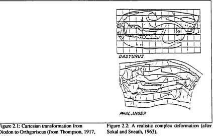
53. Figure 2.1 Cartesian transformation from Diodon to Orthogoriscus. Figure 2.2 A realistic complex deformation.
55. Figure 2.3 Two ways of describing the same affine transformation from square to rhombus.
56. Figure 2.4 Transformation of an inscribed circle into an inscribed ellipse. Figure 2.5 Change in landmark location for a triangle of landmarks. Figure 2.6 The sella-nasion-menton triangle.
57. Figure 2.7 Three ways to produce the same magnitude of angle change, by movement of different landmarks.
Illustrations
CHAPTER 3: 3D SURFACE DATA ACQUISiTION SYSTEMS FOR THE FACE
67. Figure 3.1 Moire fringes of a face.
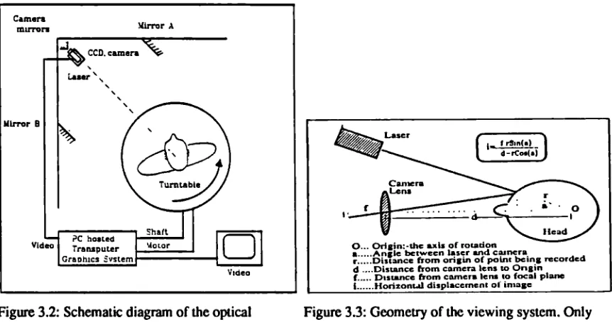
73. Figure 3.2 Schematic diagram of the UCL optical surface scanner. Figure 3.3 Geometry of the viewing system.
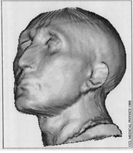
74. Figure 3.4 A rendered surface image of a bust of a Roman general
CHAPTER 4: FACIAL ANALYSIS LiTERATURE
77. Figure 4.1 da Vinci's diagram. 80. Figure 4.2 Contour plot of a face.
CHAPTER 5: CHOICE OF METHODOLOGY
93. Figure 5.1 Parabolic lines of a face.
96. Figure 5.2 Ridge and Valley lines of a face.
CHAPTER 6: DESCRIPTION OF THE FACE
102. Figure 6.1 Convolution filters for the Besi and Jam algorithm
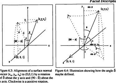
105. Figure 6.2 Effect on defined surface type with increasing window size. 107. Figure 6.3 Alignment of a surface normal vector along the z axis.
Figure 6.4 Illustration showing how the angle 8 maybe defined.
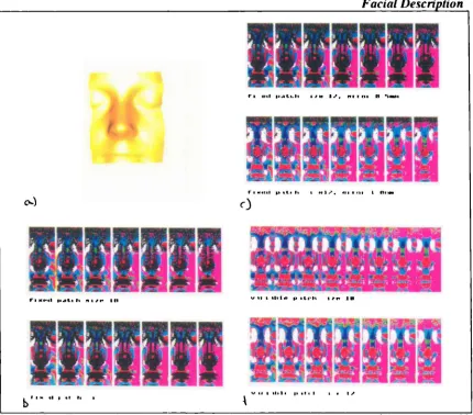
111. Figure 6.5 Test optical surface scan image and the surface type description of the image for fixed and variable patch sizes.
Figure 6.6 Smoothing of data using a low pass filter.
112. Figure 6.7 Effect of smoothing the data on the surface type description of an individual.
113. Figure 6.8 KHmap. Plot of mean curvature versus Gaussian curvature. Figure 6.9 KHmap for a face.
114. Figure 6.10 The eight fundamental surface types.
Figure 6.11 Surfaces of positive, zero and negative mean curvature, superimposed onto the optical surface scan of the face. 115. Figure 6.12 A face encoded into surface types at three different threshold
levels.
116. Figure 6.13 Variation of the total area of each surface type on one individual's face with increasing curvature thresholds. 118. Figure 6.14 Ki-I-map representations and surface type descriptions for a
cylinder and a saddle, using the Besi and Jam algorithm. Figure 6.15 Comparison of the performance of the Yoyoka and Levine
algorithm with the least squares algorithm for spheres. 120. Figure 6.16 Comparison of the surface type descriptions produced by the
Illustrations 121. Figure 6.17 The effect of size of sphere on the distribution of curvature
values.
Figure 6.18 Comparison of the surface type descriptions produced for the same face using the three algorithms.
122. Figure 6.19 Comparison of an optically scanned sphere with a simulated sphere with noise added.
123. Figure 6.20 Distribution of 100 000 randomly generated numbers normalised to represent a Gaussian distribution of noise.
124. Figure 6.21 Effect of adding random noise to a sphere. 125. Figure 6.22 Effect of adding quantization noise to a sphere.
Figure 6.23 The relative widths of normally distributed and quantization noise.
126. Figure 6.24 Surface type images and KH-maps for two combinations of normally distributed and quantization noise added to a simulated sphere.
128. Figure 6.25 Four scans of the same individual and their surface type images. 127. Figure 6.26 Variation of each surface type over the face for four scans of one
individual.
129. Figure 6.27 The effect of facial expression on the surface type description. 130. Figure 6.28 The effect of facial expression on the amount of each surface
type across the entire facial surface.
CHAPTER 7: ANALYSIS OF DIFFERENCES AND CHANGES IN THE FACE
133. Figure 7.1 Landmarks used for the registration of facial surfaces. 134. Figure 7.2 Landmarks used for the registration of facial surfaces for
patients.
135. Figure 7.3 Benson and Perrett's photographic averages.
136. Figure 7.4 Average male and female faces produced from optical surface scan data and their corresponding surface type descriptions. 137. Figure 7.5 Definitions of eyes, nose and lower face regions.
138. Figure 7.6 Graphical comparison of the amount of surface type against threshold level.
139. Figure 7.7 Summary of the comparison of amount of each surface type in three regions of the face for the average female and average male.
140. Figure 7.8 The boundary search algorithm.
Figure 7.9 Some measures of surface type patches.
Illustrations
142. Figure 7.11 List of parameters describing surface type patches on a face. 144. Figure 7.12 Example of a linguistic frame representation.
145. Figure 7.13 Example of a nose frame.
Figure 7.14 Patch locations in the nose frame.
147. Figure 7.15 Transformation of the patch centre from first image to second image.
Figure 7.16 Change in the orientation of the principal axis. 149. Figure 7.17 Production of caricatures.
151. Figure 7.18 A series of 3D caricatures of an individual and corresponding surface type images.
152. Figure 7.19 Alteration of the nose and chin using a b-spline.
153. Figure 7.20 Alteration of the nose using a b-spline, facial surface images and corresponding surface type images.
154-5. Figure 7.21 Graphes illustrating the variation of surface types with percentage of nose gradient alteration for a female face and a male face.
156. Figure 7.22 Erosion and dilation algorithm of a patch. Figure 7.23 Erosion and dilation of a patch.
Figure 7.24 Example of a patch where eroding first would split the patch. 157. Figure 7.25 The medial axis of a patch.
Figure 7.26 Erosion of the boundary to produce contours.
Figure 7.27 Possible functions used to blend the patch movement. 158. Figure 7.28 Movement of the portion of the optical surface scan image
corresponding to the right eyebrow peak and the chin peak using different blending functions.
CHAPTER 8: APPLICATIONS I:- CLINICAL
163. Figure 8.1 Cleft palate patient: facial surface images and corresponding surface type images.
164-6. Figure 8.2 Cleft palate patient: Comparison of the amount of each surface type in mid-face and lower face regions.
167. Figure 8.3 Skeletal classification. Figure 8.4 Incisor classification.
168. Figure 8.5 Le Fort lines of facial skeletal weakness.
169. Figure 8.6 Skeletal Class II patient: facial surface images and corresponding surface type images.
Illustrations 174.
175-7.
179.
180-2.
184.
Figure 8.8 Skeletal Class III patient: facial surface images and corresponding surface type images.
Figure 8.9 Skeletal Class III patient: Comparison of the amount of each surface type in mid-face and lower face regions.
Figure 8.10 Asymmetry patient: facial surface images and corresponding surface type images.
Figure 8.11 Asymmetry patient: Comparison of the amount of each surface type on the left and right hand sides of the face.
Figure 8.12 Facial growth of an adolescent boy over 2 years. Anterior view and corresponding surface type images.
185-9. Figure 8.13 Facial growth of an adolescent boy over 2 years. Comparison of the amount of each surface type across the entire facial surface and in the eyes, nose and lower face regions.
190. Figure 8.14 The definition of landmark points using the maximum curvatures of each region.
193. Figure 8.15 Examples of faces from different ages that were considered to be beautiful by people of that era.
CHAPTER 9: APPLICATIONS II: - 3D SHAPE AND FACIAL RECOGNITION
211. Figure 9.1 Faces that were rated as i) very feminine ii) sex unknown (actually feminine) and iii) very masculine.
212. Figure 9.2 Comparison of the amount of peak (left), minimal (centre) and saddle valley (brown) surfaces in the nose region for faces that were rated as very feminine, very masculine and of indistinct sex (actually female).
215. Figure 9.3
216-7. Figure 9.4
Facial surfaces images and corresponding surface type description for faces rated as i) distinctive male ii) distinctive female iii) typical male iv) typical female.
Comparison of the amount of surface types in three regions of the face for male (left) and female (right) faces rated as distinctive, typical and average.
APPENDIX A: EQUATIONS OF FUNDAMENTAL SOLIDS
QUOTATION
"Had Cleopatra's nose been shorter, the whole face of the world would have been different."
ACKNOWLEDGEMENTS
Like most theses, this work has been started but not completed. However, the fact that it has reached this point or even that it was begun at all, is due the important contributions of many people. It this therefore my pleasure to begin the writing of this thesis by thanking them all.
Firstly, I should like to thank Dr. Alf Linney, not only my supervisor for this work but a great friend, who has been tireless in his encouragement and support during the past 5 years. It was the invention and development of the optical surface scanning system by Dr. Linney, Prof. Moss and others in the Department of Medical Physics that enabled this work to be undertaken and he has made numerous valuable suggestions on the direction of this work as well as its content and presentation.
My thanks to all the members of the Medical Graphics and Imaging group at Department of Medical Physics, University College London for all their support and help. In particular, this thesis owes a lot to Dr. Robin Richards who has been extremely patient with all my questions about OCCAM programming, the Transputer development system (TDS) and the data format. He has also provided me with a lot of help regarding the design of algorithms, debugging and helped me clarify my ideas, read portions of this thesis and provided lots of encouragement. Dr. Rick Fright's work on a 3D registration technique, the construction of average faces and caricatures has enabled me to make the comparisons described in chapter 7 between faces. Rick is now at Christchurch Hospital, New Zealand. Thanks also to Joafl Campos for helpful discussions about scale space analysis.
An important influence in this work has been the collaboration from October 1989 to July 1992, with the Department of Psychology at Nottingham University. I have very much appreciated the wonderful enthusiasm and encouragement of Professor Vicki Bruce and Dr. Mike Burton (both now at the University of Stirling) for this work and I am grateful to Professor Bruce for her helpful comments on chapter 9 of this work. Dr. Elias Hanna provided me with 3D data altered by B-splines to produce the nose and chin shape changes analysed in chapter 7.
Acknowledgements
Chapter's 4 and 8 and to Trid,.a Goodwin (UCL, Medical Physics) for providing me with details of the operations analysed in chapter 8.
My thanks to Dr. Peter Williams ((JCL., Mathematics) for a useful discussion concerning the least squares surface fitting algorithm and to Professor Kanti Mardia (University of Leeds, Statistics) and Professor Fred Bookstein (Center for Human Growth, Ann Arbor, Michigan) for helpful discussions regarding statistical analysis of the surface type data. Thanks also to Dr. Robert Speller for his advice concerning the structuring of this thesis and to Andrew Todd-Pokropek for reading it through and his comments which have helped make it a more cohesive whole.
Thanks to Dr. Gaile Gordon (now at The Analytical Systems Corporation, Reading, MA formerly at Harvard Robotics Lab.) for useful discussions regarding the use of surface type descriptors and to Dr. Su-Shing Chen (National Science Foundation and University of North Carolina, Mathematics) for his encouragement.
My family and friends have been a great support, encouraging me to get on and write this, whilest at the same time ensuring that I stayed firmly in the real world! Special thanks to Mum and Dad, Emma Page, Mary-Jane Pownell, Janice Kennedy, Graham Caws and Geoff Dobson. In the early years of this work, my mother looked after me, enabling me to get on and write this without the distractions of washing, ironing and cooking!
INTRODUCTION
The face is a dynamic structure, unique to the individual and plays a very important role in recognising individuals and in attracting us emotionally, socially and sexually to an individual. It also plays an important role in portraying our emotions, signaling changes in mood and communicating feelings (Gorlin et al, 1975).
Motivation for a description of facial shape
The study of the face is important to many different scientific and medical disciplines. Changes in facial appearance due to normal growth, abnormal growth, injury and surgery can and do have a profound effect on the person concerned. The psychosocial consequences of having to spend a significant portion of one's childhood with a major uncorrected facial malformation can be devastating (Cutting, 1989) whereas the surgical correction of facial deformity often gives a person more self-confidence and a less introverted personality. If facial surgery is to produce a consistent Outcome it is necessary to have an objective means for describing facial change and to relate this to an assessment of the outcome. This requirement has led to many attempts being made over the years to measure and characterize changes in facial shape. The research described in this thesis arose from this need.
During the last decade computer systems have been increasingly used in the planning of facial surgery. A number of such systems have been developed including one at University College London (Arridge et al, 1985; Moss et al, 1988; Tan et al, 1988; Linney, 1992a; 1992b). These modern systems use computer graphics to provide the necessary three dimensional (3D) representations of the facial surface. They enable the face to be displayed as seen from any chosen viewpoint and allow the data to be manipulated to simulate the effect of surgery. The availability of computed, stored 3D data has opened up the possibility of a mathematical analysis and description of the facial surface.
A mathematical description of the face is also very important in research into facial recognition. In her book, "Recognising faces", Bruce reviews the research conducted by cognitive psychologists into this subject (Bruce, 1988). Much of the work in this field to date has been conducted on two dimensional images of the face. Bruce concluded that further understanding of the way in which we recognise faces, is dependant on treating the face as a 3D surface not a 2D pattern. This concept has provided a second motivation for this work.
Introduction
used, although not well defined. I have therefore sought to produce a mathematical description of the face based on its shape.
Most of the mathematical methods which have previously been applied to facial analysis have been based on landmark points. These must first be accurately identified. Analyses have, for the most part, been limited to studies of the midline profile. Since most of the face consists of surface in between landmarks these methods of analysis represent a very high degree of abstraction. The application of landmark analyses to the
characterization of facial change fails completely for cases in which the landmark points chosen have been moved only slightly or not at all but the perceived change in the facial shape is extremely marked.
What is shape?
The question of How should we describe shape? is a question often dismissed as trivial
but in fact, it is hard to answer precisely. Kendall (1989) has suggested one plausible definition of shape; that it is "what is left over" when the effects resulting from translations, changes of scale and rotations are filtered out. It is immediately apparent is that any objective description of shape (or form) must use only parameters for comparison which are independent of orientation (rotation), translation and linear scaling. Intuitively is seems that shape is to do with curvature.
The Oxford English Dictionary definition of shape is "the total effect produced by a thing's outlines". This is difficult to translate into an exact mathematical definition. In formulating a theory for shape, the properties associated with shape must be deduced. This is not an easy task. In 1967, Blum observed that the properties of shape have proved difficult to deduce primarily because "the number and variety of shapes are enormous" (Blum, 1967). A great deal of research has been done on the description of
shape per se and associated computation methods (see chapters 1 and 2) but it is clear
from the literature that the characterisation of facial shape and mathematical description of changes in facial shape have, apart from a few notable examples, been lacking. This is the subject of investigation in this work.
Introduction Purpose
The purpose of this work has been to produce a surface-based description of the shape
of face and to explore methods of characterizing changes in the shape of the face. Requirements are that the description is based on the entire 3D structure of the face, is invariant to the viewpoint from which the face is observed, robust against noise and repeatable for scans of the same face. It must also enable a quantitative comparison of the 3D changes in the face to be made that is explicable in terms of the perceived changes or differences. The description and the comparison of changes should be amenable to automation, so that they can be implemented for practical applications.
CHAPTER 1
SHAPE DESCRIPTION - LITERATURE REVIEW
In this first chapter, a brief review of the literature dealing with the description of shape and especially 3D shape is given. There has been an abundance of literature produced over the last two decades relating to shape description, much of which is in a similar vein. I have therefore been somewhat selective in referencing papers, seeking to point
to authoritative texts describing a particular approach or idea or quoting an example of
that approach, whilst endeavouring to still do justice to the ideas advanced by those scientists interested in this subject.
Cognitive psychologists have proposed a number of theories for describing the manner in which our visual system perceives shape and how our concepts of shape are formed (Bruce and Green, 1985). These have been intrinsically bound up with how we recognise objects (see chapter 9 for psychological literature pertaining to the recognition of faces). Apparently independent of this, scientists working in the computer vision field have produced various descriptions of shape which seem to be based on somewhat similar concepts. However, until the last few years there has been very little cross-referencing found in the literature. The computer vision approach to shape description uses ideas of image segmentation, feature extraction, artificial intelligence and differential geometry. The role of shape description in computer vision is to enable the recognition of objects, or scenes of objects, primarily for robotic applications. This role ties in well with one of the goals of cognitive psychologists, trying to understand how we recognize objects. In this chapter I will attempt to relate the approaches taken by these two fields. The material described here is of importance for the development of a method for describing facial shape.
Separate from these approaches has been the long history of interest in biological shape which stems, in modern times, from Darwin and his ideas about evolution. Early attempts to formulate biological development and evolution in terms of shape were made by D'Arcy Thompson in his classic work "On Growth and Form" of 1917 and emulated by others (eg. Richards (1955)). More recently Bookstein (1978a; 1978b) returned to Thompson's work and extended it. The aim of their work was the classification of changes in shapes, rather than the development of a description or concept of shape. Therefore this will be discussed in a separate chapter along with the statistical analysis of shape (chapter 2).
LI. Human visual perception
Shape Literature discover how the cognitive system works, quickly led them to form concepts of how the brain might describe shape. Considering a mathematical description of shape there is an intrinsic advantage claimed for using a conceptual model of shape based on the mechanisms of the brain's visual system, that is that the system is known to work! Let us now consider how shape may be represented in the brain.
1.1.1 Observations about the brains perception of shaDe
It has been found that the perception of an object's shape enables us to identify that object and that this is true whether or not the object is rigid, since living things are just as easily recognisable as non-living ones (Attneave, 1967). So the perception of shape facilitates recognition.
Psychologists have made a number of basic observations about how we perceive shape. Psychophysical and neurophysiological experiments have found that different areas of the brain respond to djfferent shapes and that shape outlines and the negation of a simple shape excite different areas of the visual cortex (eg. Perrett et al, 1988). Shape in the visual cortex seems to be mainly feature based and curvature along a curve or contour may be a key descriptor (Dobbins et al, 1987; Leymarie and Levine, 1988; 1989). This would explain how objects can be recognized from their silhouettes or outlines (Marr, 1977).
Regarding the perception of faces, clinical and experimental studies have shown that there are cells in the inferotemporal cortex of monkeys which specifically respond to faces (Tanaka et al, 1991). In man too there appear to be cells that respond specifically to faces and the neural mechanisms for face processing are predominantly, but not exclusively, located in the right cerebral hemisphere (Perrett et al, 1988).
Next, we can recognise objects when they are seen from different viewpoints or in different states. For example, a face can be recognised when seen from in front (anterior view), obliquely or in profile (lateral view) and with different facial expressions. It has been shown that faces are most easily recognisable as belonging to a particular individual when seen in three-quarter view and that profiles are less easy to recognise, unless the individual face is a very distinctive one (Bruce et al, 1987). It has been found that in the brain, different cells are excited by the same shape in different orientations or, in the case of a face, when portraying different emotions (Perrett et al, 1988).
Shape Literature
interconnection with language area of the brain. We can also assign features to an object, or segment an object into parts. Facial features such as the nose can be recognised although it is contained within a Continuous surface and varies enormously from individual to individual and race to race. Just how we can make such a distinction is still unknown.
The perceptual process is reversible. That is to say that we can somehow store the salient information about an object to enable us to recall it, and draw it from memory, at a later date. This recall ability appears to be influenced by our familiarity with the object, the importance of the object to the individual and the passage of time since its observation. It has been demonstrated that if one is asked to visualise an object, such as a cat, one visualises a specifIc breed of cat, which may vary from individual to individual (Attneave, 1967). These observations suggest perception is strongly dependent on learning. It also implies that information is abstracted from the retinal image and compressed for storage. Other observations suggest that incoherent information is discarded and only features of high informational value is retained (Attneave, 1954), as well as a preference for simple features over complex ones.
When we considering an image of an object, our interpretation of the image seems to be influenced by environmental cues such as vertical and horizontal orientation (eg. the distinction we make between a square and a rhombus), right angles, parallel lines leading to vanishing points and viewpoint. Highlights appear to reinforce the interpretation of surfaces (Blake and Bülthoff, 1991). Stevens (1981) showed that a localised highlight suggests an elliptic surface is being viewed whereas a linear, elongated highlight suggests a cylindrical one. The background surrounding an object appears to have little effect on how the object is perceived. However, if one reverses components of an object, great difficulty arises in identifying the object (eg. figure 1.1). This suggests that our perceptual sense is finely tuned.
¶ W •
Shape Literature If a percept is often used or is important, such as recognizing familiar faces, a special-purpose mechanism, entirely for that task is developed by the brain. Thus expert descriptions are formed differently from those of naive observers. Computer simulations of expert descriptions require the construction of more specialized models than those for naive observers. All adults are experts at recognizing faces (Diamond and Carey, 1986)
Figure 1.2: Boring's figure. An example of "figure-ground reversal", seen as either a young girl or an old woman.
As long ago as the 17th century, people noticed that under certain circumstances, ambiguity exists in the way that the human visual system perceives shape. That is to say that some line drawings, or shaded line drawings, can be interpreted in two mutually exclusive ways. This phenomenon is termed "figure-ground reversal". Boring's figure (figure 1.2), which can be seen either as a mother-in-law or a wife, is a famous example of this and there are many others.
The psychological experiments that have been conducted in order to investigate the perceptual organisation of the mind, often use the manner in which people "see" 2D contours or figures to examine how shape is perceived. These have not only provided some important observations about the perception of 2D outlines (which I shall call "contours") but have led to the formation of a concept of what the "same shape" is and, importantly, inferred that shape is amenable to mathematical description.
Shape Literature
figure made the figure less recognizable than changing its size they concluded that sense was more important as a recognition factor than size.
>1
- __ $mI,. SS.e(doS)
od_ -
C-Figure 13: The "sense" of a figure. clockwise and anti-clockwise.
1.1.2 Perceptual representation of shape
The observations described above tell us that the perception of an object's shape is bound up with its recognition. They have also provided some important pointers about how we perceive shape, helping us to develop concepts of what shape is. But how does the brain abstract this shape information from its visual input?
This has also been a subject of considerable interest, a review of research describing the perceptual representation of form with a view to defining mathematical metrics for describing shape was given as early as 1965 (Michels and Zusne, 1965). Two main theories have been advanced to explain how the shape information is encoded. In this section, I shall firstly describe these two theories and in the next section briefly review algorithms devised by computer vision scientists which have used these concepts.
a) Shape from edges
The first theory is rooted in the observation that artists will often make a preliminary sketch of a scene before painting it. This sketch is essentially a line drawing from which the scene can be recognised without any visual cues such as shading, colour or texture. The line drawing has been defined as the minimal representation of intensity discontinuities in a grey-level image that adequately conveys surface structure (Barrow and Tenenbaum, 1981). The identification of such lines with high frequency changes in intensity in the retinal image (see Bruce and Green, 1985) led to a theory which suggested that the human visual system works as a high-pass filter, capable of detecting edges and deducing shape information from them (Grimson and Pavlidis, 1985).
Shape Literature tangent in the plane of the space curve (Barrow and Tenenbaum, 1981).
It was Marr who suggested that because intensity discontinuities would often coincide with important boundaries in the visual scene, these edges are stored by the brain as a symbolic two dimensional representation of the object, a primal sketch (Marr, 1976;
1982). This representation is also supposed to record the turning points in curved edges (ie. changes of sign of the second order partial derivatives of curves) and the contrast, blur and local orientation of edges (by filtering the image with different size gaussian functions) (Marr and Hildreth, 1980; Marr and Poggio, 1979). A more complete viewer-centred representation, which Marr called a 2'12 D sketch, was obtained by combining
depth, motion and shading information with the primal sketch. This describes the layout of structures in the world from a particular viewpoint.
For natural scenes, the changes in light intensity associated with the edges of objects are embedded within the changes caused by surface texture, shape, shadows and arrangement of illuminating light sources (Watt, 1988). This makes any correspondence of intensity changes to the edges of objects difficult to ascertain.
Some psychophysical evidence has been obtained to suggest that the human visual system does uses a kind of primal sketch (Watt, 1987a; 1987b). However, compared to Mar? s primal sketch it is of a more dynamic and structured nature (Watt, 1987c). Marr and Hildreth's algorithm detects edges in an image scene by convolution with a range of different sized Gaussian filters and uses zero-crossings (ie. points of inflection) in the second directional derivative to locate edges. Pearson and Robinson (1985) found that for faces using the peak response of the filter produced a better edge description than using the zero-crossings. Watt and Morgan (1985) devised an algorithm called MIRAGE to simulate more closely the working of the human vision system and to allow any changes in image intensity to be described.
When assessing the usefulness of the concept of edge detection to us, we should consider that line drawings of objects do contain a lot of psychologically salient information (eg. figure 1.4) and a qualitative appreciation for the shape of a surface can be obtained from a line drawing. Some idea of its orientation is also relatively easy to judge, but its size is not (Stevens, 1981). Barrow and Tenenbaum (1981) have pointed out that the outline of a structure appears to influence the brains perspective and motion parallax cues (such as the Necker cube which is seen to reverse in depth, figure 1.5).
' k
Shape Literature
drawings of the faces of individuals, have been shown to be inadequate for facial recognition (Bruce et al (in pressa), see also chapter 9.1.1).
Figure 1.4: A line drawing of a face. Surface and Figure 1.5: Necker's cube, which undergoes boundary structure are perceived, spontaneous reversals in depth.
Mathematically, this sort of edge-based description is inadequate because it is not invariant under monotonic transformations and it assumes that the general structure of an object is isotropic and smooth in order to obtain useful information. In the real-world this is often wrong. The well-documented figure-ground reversal observation provides evidence against the edge based theory. Consider Rubin's figure (first reported by Turton in 1819 referenced by Hoffman and Richards, 1985) which can be seen either as two faces or a wine goblet (figure 1.6). In 1915, Rubin found that if one sees the figure in one way, then later in the other way, he is no more likely to recognise the figure than if he had never seen it. Thus the relationship between the two drawings is in some sense "competitive". This suggests that object recognition is not solely do to with the contour properties, for if this were the case it should not matter which side of the contour the object is perceived to be.
L11 L]
Figure 1.6: Rubin's figure, seen as left: a goblet, by defining part boundaries at curvature minima corresponding of the base, stem, bowl and lip or right: pair of facing facial profiles, by the curvature minima corresponding to nasion, nose base, lips and chin.
Shape Literature
b) Shape as parts
The second theory of how shape is represented in the visual system is complementary to the first. It is that the brain decomposes shape into parts in order to facilitate recognition. This idea helps to explain how objects can be recognised even though they may have some components missing or are seen from a number of viewpoints. It also takes account of motion. The question then arises as to how the brain segments an object into parts and whether the same strategy can be applied computationally. One consideration is that the parts must be invariant with time and viewing geometry (Marr and Nishihara, 1978).
In two dimensions, the points of curvature inflection of a contour have long provided a natural and useful method of segmentation. They also appear to have some psychological meaning. In 1954, Attneave (1954) estimated the points of highest curvature on a photograph of a cat. He drew a line drawing connecting these points from which he was still able to recognise the cat. He therefore surmised that these points must have a high information content.
Suggestions of how the visual system defines part boundaries have included segmentation at inflection points (Hollerbach, 1975; Marr, 1977), segmentation at points of maximum and minimum curvature (Duda and Hart, 1972) and segmentation at points with tangent and curvature discontinuities (Binford, 1981). Another hypothesis was that the visual system divides surfaces into parts using the loci of zero Gaussian curvature (ie. parabolic points) (Koenderink and van Doom, 1982). This latter hypothesis was convincingly rebuked in theory by Hoffman and Richards (1985) and intuitively by considering the parabolic lines marked on a bust of Apollo Belvedere by the famous German mathematician Klein (1-lilbert and Cohn-Vossen, 1952) where these lines seem to have no perceptual meaning.
Hoffman and Richards (1985) hypothesized that a rule from differential topology called "transversality regularity" is used by the visual system to segment a surface into parts. This rule is based on the observation that when two surfaces intersect they always meet in a contour of concave discontinuity in their tangent planes. Accordingly, surfaces are divided into parts along all contours of concave discontinuity of the tangent plane. Using differential geometric concepts, they show that smooth surfaces are divided by the loci of the negative minima of each principal curvature. The concepts of differential geometry are discussed further in chapter 5.
Shape Literature
maxima and vice versa. Therefore the part boundaries change and the figure is seen in a
different way.
I tested this theory by conducting a small experiment. I asked 10 individuals to divide the curve shown in figure 1.7 into parts. All segmented the curve at points B,D,F,H, and J - the negative minima and not at points A,C,E,G and I - the positive maxima. When the figure was inverted all subjects segmented the curve at points A,C,E,G, and I. Thus this theory was verified.
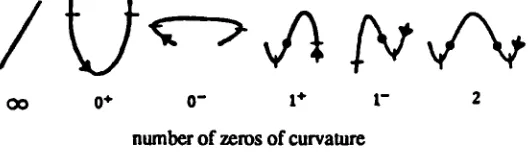
For 2D curves, Hoffman and Richards (1985) derived six shape primitives, or "codons", terminated at points of negative minima and marking part boundaries (figure 1.8). There are only six possible ways in which a curve can vary between two negative minima. The segmentation of an object in this manner has been done intuitively by those seeking mathematical descriptions of curves and contours.
Figure 1.7: Segmentation of a profile at the points of negative minima in curvature.
00
r
2number of zeros of curvature
Figure 1.8: The "codons" of Hoffman and Richards. Zeros of curvature are indicated by dots, minima by slashes.
The full implication of this theory for surfaces is described later in this chapter. But first I shall discuss the methods which have been used to describe shape in two dimensions mathematically, since some useful concepts have resulted from these descriptions, which descriptions of 3D shape have built on.
L2
Mathematical descriDtions of 2D contoursShape Literature up" methods respectively. Local features have been demonstrated to play an important
role in shape analysis (Rosenfeld and Johnson, 1970; Rosenfeld and Weszka, 1975), but for recognition purposes the whole shape must also be considered. In practice, a mixture of local and global methods often seem to give the best, fastest and most reliable descriptions. Multiple-scale, or hierarchical, representations have recently become an important part of any successful shape description because they allow the shape to be described both locally and globally.
For any representation of shape to be useful, it must be a shorter description (ie. have a smaller storage requirement) than the original shape and yet still contain the essential characteristics of the object's shape for it to be recognisable. Multi-level representations suppress surplus information to achieve this requirement (Hollerbach, 1975).
Throughout the literature pertaining to the mathematical description of 2D shape (outlines) the terms "contour" and "boundary" are liberally, and confusingly, interchanged. I shall use throughout the term "contour" to mean a closed (bounded) form and "boundary" to refer to the actual boundary of the form. The methods used for describing these 2D abstractions mathematically are now reviewed.
1.2.1 Description and classification of 2D contours
The attempts made by scientists working in the computer vision field to find suitable descriptions of contours have been motivated by the desire to recognize such contours quickly and easily for a variety of tasks which range from industrial quality assurance to the recognition of aircraft outlines for defence purposes (Wallace et al, 1981). The first techniques that were developed for examining the shape of 2D contours subscribed to the part theory, describing the boundary in terms of segments. Syntactic methods could then be used to describe the boundary string. However, the computational expense of this approach prompted researchers to look for means of reducing the information content of the description. Decomposing the contour into parts (Shapiro, 1980) or deriving some sort of statistical measure was one way of doing this (see section a). Another approach was to extract properties of the contour, such as the medial axis or its representation in scale space (see section d), and use these to classify its shape.
a) Description of the bounding contour
Shape Literature
The segmented boundary has been approximated by various functions to enable it to be quantified. Attneave (1954) used spline functions, but later iterative fitting methods were used to obtain a more accurate description. One of the first of these used circle segments (Shapiro and Lipkin, 1977) but this required many iterations to achieve a good match and produced many small segments. (Incidentally, these authors suggested that this technique could be extended to 3D using spherical segments but this would be an extremely expensive operation computationally and the subsequent matching of segments would be difficult.) A natural progression was to use polynomial functions to approximate the contour, iteratively refining the function until the error of fitting was lower than some threshold (Wallace et al, 1981).
A second description of the boundary used pattern recognition techniques to provide a syntactic description (Fu, 1974; Pavlidis, 1978). These can be quite complex and encounter the problem of closing incomplete boundaries, although this problem can be overcome by developing the syntactic description only up to a certain level (ie. using local properties) (Horowitz, 1975). Another difficulty was that noise in the data lead to the production of such complex syntactic strings that for some contours it becomes necessary to use a string containing the entire set of boundary points! Successful syntactic descriptions have been those which stress local aspects of the contour. However, these approaches enabled a language (or grammar) for describing shape to be defined, in terms of arcs, lines, protrusions etc., which is governed by semantic rules. The probabilistic or fuzzy character of the grammar often makes the governing rules appear to be unrealistic, but they contribute a flexibility to the approach which allows them to succeed. Hierarchical syntactic descriptors such as Pavlidis' (1979) have overcome some of these problems but are again computationally expensive.
Our ability to recognise an object from its silhouette, and hence its boundary, inspired Asada and Brady's (1986) curvature primal sketch. In this representation, the boundary
s symbolically described using a set of curvature change primitives. Significant changes in curvature along the contour's boundary were represented in a similar manner to the intensity change representation of Marr (1976; 1982). A multi-level approach was adopted, in which the curvature changes are located at the finest level of detail at which they can still be detected. The greater the number of scales at which the curvature changes are detected, the more global a descriptor of shape the change is. This was extended to 3D by Ponce and Brady (1985) to describe significant surface changes (described later in this chapter on page 48).
Shape Literature (1979). A statistical distance measure computed between the vectors facilitated
recognition. Such representations have also been used to recognise objects from their partial boundaries (McKee and Aggarwal, 1977; Ansari and Deip, 1990). This requires an estimation of the closeness of match between the representation of a particular contour and the representations of a known contour stored in a "library". Leu (1989) observed that the recognition of objects from their boundary, becomes ineffective if the object is seen from a skewed angle, hence a normalization algorithm is needed to standardize the contour in order to facilitate recognition.
b) Mathematical morphology
A very different approach for accurately extracting the boundary was devised by Matheron (1975) at the Ecole des Mines de Paris, and became known as mathematical morphology. The context in which it was developed was cellular automata and the connection between cellular arrays, retinal devices and image processing architectures have prompt considerable activity in this area (Skolnick, 1986).
In this method, the images being analysed are considered as sets of points and operations defined by set theory are used to describe the boundary (Serra, 1986). The method is different from other image processing techniques because it is based on the logical relations between points rather than arithmetic ones. It provides a means of decomposing global geometric measurements into sequences of local transformations. Different algorithms are specified by the different neighbourhoods of points defining these sequences of transformations. It begins with a "hit or miss" transform which defines whether a point on the boundary belongs to the enclosed object (the contour) or to the enclosing object outside of it (Serra, 1982; 1986) and proceeds with erosion/dilation transforms to build up a useful set of image processing algorithms such as skeletons and various filters (Skolnick, 1986). Mathematical morphology has been successfully applied to grey-scale images for the extraction of features (eg. Archibald and Sternberg, 1986). However, the algorithm is sensitive to lighting conditions for the scene under analysis. This method has also provided a decomposition of a contour into a union of simple components that is unique and invariant to translation, rotation and scale (Pitas and Venetsanopoulos, 1990).
ci Viewpoint invariant descriptions
Shape Literature
Persoon and Fu, 1977)) specifically address one requirement for the description of an object's shape. That is that the description is independent of object location, orientation, and viewpoint.
Moment invariants are so called because they are invariant with respect to rotation and scale change. The accuracy of the representation they produce depends on the number of moments used, but of course the greater the number of moments, the longer the computational time. They have been used to match scenes of objects (Wong and Hall,
1978). Originally applied to 2-D scenes, Sadjadi and Hall (1980) extended them to three dimensions, but these do not seem to have been used by others.
In the case of globally applied Fourier descriptors, no clear relationship between the representation and human perception is seen for the representation is unable to make the distinction between a square of side x and a circle of diameter x (Pavlidis, 1978). However, segments of boundaries have been described fairly successfully using Fourier descriptors calculated from chain-coding (Gorman et a!, 1988). An advantage of this description is that the Fourier descriptors are independent of size, orientation, starting point and can be employed to recognise partial contours. They have also been used to recognize aircraft outlines (Wallace and Wintz, 1980; Arbter et al, 1990) and handwritten numerals (Persoon and Fu, 1977) via the extraction of skeletons, somewhat similar to medial axis representations (see section di). Other functions that have been used in a similar fashion include Walsh functions (Searle, 1970) and the rapid transform (RT) (Reithoeck and Brady, 1969).
A novel attempt at describing 2D convex shapes was the superimposition of a hexagonal 3 axes grid on the shape (Greene and Waksman, 1987). The hexagonal structure is based on the structure of the eye's visual receptor cells. The number of occluded grid points along each axes was used to measure the distance through the shape and the frequency of these occurrences compared with the distance through the grid gives a unique signature for the shape. The method reveals the difference between
regular shapes such as squares, triangles and circles but appears to be totally
unintelligible for irregular shapes. Another drawback is that it is not invariant to rotational changes. Interestingly, the authors claim that this
is
consistent with human perception as we perceive shapes differently when viewed from different angles, that is the same shape maybe seen as square or rhombus.d) Extraction of information from the boundary
ii Skeletal representations
Shape Literature however, be regenerated from these skeletal representations. But if the skeleton is unique, it may nonetheless be used for recognition purposes.
The three approaches are the smoothed local symmetries representation (SLS), the symmetric axis transform (SAT) and process-inferring symmetry analysis (PISA). The difference between them lies in their definitions which are closely related and illustrated geometrically in figure 1.9. The SAT is the locus of the centre 0, SLS the locus of the midpoint P of the chord joining A and B, where A and B are the points where the maximal disk intersects the contour and PISA is the locus of the point Q, the midpoint of the arc AB. For a detailed comparison of these algorithms see Rosenfeld (1986).
Figure 1.9: Geometric definitions of the SAT, SLS and NSA. Curves C 1 and C2 have tangents vectors at A and B. The SAT-axis is the locus of circle centres 0, The SLS the locus of points P and PISA-axis the locus of points Q.
Symmetric axis transform (SAD
The Symmetric Axis transform (SAT) is sometimes known as the medial axis transform, the term its inventor Blum used (Blum, 1967; 1973). Blum defined the medial axis of a contour by considering the brain's interpretation of wave fronts being propagated outwards from the centre of the shape and either exciting or inhibiting sensors placed in the field around it. These sensors could only be fired once and were unaffected by a second wave front passing through them. "Corners" occurred in the wave front contours at the minimum radius of curvatures and the locus of these corners defined the medial axis. A medial axis function was defined as the number of times a corner occurred on the medial axis.
Shape Literature
1977). This function is an unique, and invertible, transform from the original form to the medial axis. Another way to define this representation is as the union of the centres of maximal disks that touch at least two points of the boundary of an object (figure 1.11). The symmetric axis is the locus of the maximal disks centres.
Blum and Nagel (1978) made a generalisation of the original form of the algorithm which reduced the effect of noise on the algorithm and the medial axis transform was more robustly defined for grey-level images by Moore and Seidl (1974).
Figure 1.10: Formation of the medial axis by consideration of a contour being collapsed inwards at constant velocity (adapted from de Souza and Houghton, 1977).
Figure 1.11: Formation of the medial axis by consideration of the locus of the maximal disks that touch the boundary at two points. (adapted from Brady, 1983).
Some advantages of the medial axis representation are that it is continuous and eliminates the need for the contour to be in a particular orientation when analysing its shape. The representation contains a local symmetry definition, is information preserving (Blum, 1973 p.216) and unique for a contour. The branching structure of the axis enables components of the shape to be defined and there is some evidence that human eye movements are related to the medial axis function of a line drawing (Richards and Kaufman, 1969).
Shape Literature Smoothed local s ymmetries (SLS
The smoothed local symmetries representation (SLS), proposed by Brady and Asada (1984), represents a contour using the locus of the midpoint of the chord joining the points A and B on the bounding contour. The SLS is a more comprehensive descriptor than SAT. For instance, for an ellipse, the SAT finds only the major axis whereas SLS finds both the major and minor axes (Leyton, 1987b) (figure 1.12). The description produced is closely related to the generalised cylinders description for 3D objects, discussed later (Nevatia and Binford, 1977; Brooks, 1981).
Figure 1.12: SAT and SLS representations of an ellipse and a rectangle.
Recently, Cho and Dunn (1991) have described a modification of the SLS called Hierarchical local symmetries, HLS, which excludes non-intrinsic and redundant local symmetries and enables a hierarchical decomposition of information based on local symmetry. The axis information is organised by the tangent difference between two boundary points forming a local symmetry. Rom and Medioni (1991) have proposed a similar hierarchical description of shape based on the SLS which allows the identification of parts of a contour.
Process-inferring symmetry analysis (PISA')
The third skeletal type representation was described by Leyton (1988). Termed process-infering symmetry analysis (PISA) it consider shape to be the result of some historical process. Curvature extrema are obtained by using the "symmetric axis-curvature duality theory" (Leyton, 1987; Yuille and Leighton, 1987). This theorem states that "any segment of a smooth planar curve, bounded by two consecutive curvature extrema of same type has a unique differential symmetric axis which terminates at the curvature extrema of opposite type" (see figure 1.13). This idea is used, but not explicitly stated, in the SAT description.
Figure 1.13: Symmetric axis-curvature duality (adapted from LeyLon 1987).
Shape Literature
Recently, a new method for obtaining the skeleton of a contour, based on active contours (or "snakes" (Kass et al, 1987)) has been proposed by Leymarie and Levine (1992). Leymarie and Levine argue that using the boundary information together with a contour's skeleton produces a richer, more powerful and efficient shape representation. Boundary information is included into the algorithm by the extraction of curvature extrema and arcs of constant curvature.
Multiresolution SAT description
The characterization of changes between two contours requires an assessment of their overall similarity in shape. This involves measurement of the importance of each component of the contour. The multiresolution approach of Gauch, Pizer and their colleagues addressed this question (Gauch et al, 1987; Pizer et al, 1987; 1988). Here, 2D contours are obtained from a grey-scale image at different levels of intensity and the medial axis of each contour is extracted using the SAT. The importance of each branch of the medial axis is determined by its annihilation by, or of, an adjacent branch as one tracks the branch from low to high scales. Thus a hierarchical structure is imposed onto the axis branches allowing branches to be considered as sub-objects of one principal axis. In this hierarchy, termed an "axis pile", the width of the medial axis function and the axis of symmetry are used to characterize the contour.
This technique has been applied to analysis of the shape of jaws by simplifying the analysis of mandible outlines and was able to reveal differences between two types of jaw. However, a large storage capacity is required and the process is computationally expensive (Pizer has quoted times of half an hour to perform the necessary calculations for one representation).
Pizer also described another method called "vertex curves" in which vertices of one contour ("level curve") are followed to the next producing curves on the image surface. These curves supply boundaries to segment the image into "codon districts" and multiresolution analysis of these districts gives a representation which describes the spatial curvature properties of the image as a function of scale. Both this and Nackman's description give information about the shape of grey-scale images at various levels. Pizer and colleagues applied these techniques to the analysis of medical images (Pizer et al; 1988).
Shape Literature Multiresolution techniques such as these have been shown to improve the segmentation of an image over established techniques based on local pixel properties or edge strength (Lifshitz, 1987). The association of pixels to components of shape is crucial for this segmentation. Gauch et al (1987) postulated that if the multiresolution SAT could be used to impose pseudo-landmarks onto an image then a biorthogonal grid deformation analysis (Bookstein described later) might be used to describe morphological changes in soft-tissue surfaces where recognizable landmarks do not exist.
ii) Scale-space method
Another method for describing contours by extracting information from the boundary
was Scale-space filtering (Witkin, 1983). In this method, a signal or curve is
successively filtered with a Gaussian mask of varying widths. This introduces a scale parameter. The curvature of the filtered signal is measured and the inflection points or "crossings", where the curvature changes sign, determined at each scale. The zero-crossings are used to form a hierarchical description of the signal which is termed a "Scale-space Image" which contains information about the location and extent of features in the signal. An example for a facial profile is shown in figure 1.14. By applying a stability criteria, events which persist throughout the scale-space can be identified as major features of the curve.
The Scale-space image can be reduced to a simple tree structure by the relation of the contours, formed by the zero-crossings, to one another as parents and children. For these branches to be stable, a stability test is needed. Witkin developed a suitable stability test based on the correspondence between intervals of the signal and their perceptual salience (Witkin, 1983).
Shape Literature
Witkin automatically determined a discrete set of scales which were useful symbolic descriptors of the curve and these were later interpreted in terms of primitive events by Asada and Brady (1986). Yuille and Poggio (1983a) found that the contours formed from zero-crossings of the second derivatives might have enough information content to enable their use in reconstructing the original signal to within a constant scale factor. They also found that the Gaussian convolution filter has the unique property of not introducing extraneous zero-crossings as one moves from fine to coarser scales (Yuille and Poggio, 1983b) and is, as such, "well-behaved" mathematically.
The Scale-space representation is sensitive to the amount of change made to the curve, except in the instance of a very small, very convex change being made. It is computationally efficient and not influenced by arbitrary choices made (such as starting point). Apart from for convex shapes, which have no zero crossings since the curvature is always positive, it is a unique representation for a curve. Mokhtarian and Mackworth used curvature, computed at various levels of detail by convolution of the path length parameters with a Gaussian kernel. They refined this method by reparameterizing each convolved curve by its normalized arc length parameter (Mackworth and Mokhtarian, 1988). This "renormalization" is equilivalent to a continuous, non-linear horizontal shear of the scale-space image. It is more suitable for matching similar shaped curves in the presence of noise.
Rotem and Zeevi (1986) succeeded in recovering the original 2D signals from their zero-crossings thereby showing that no information is lost by working in scale-space. Bischof and Caelli (1988) maintained that scale-space is only useful in terms of what it can tell us about shape in conjunction with other methods, demonstrating how it can improve the shape-from-texture method (see section 1.4.1 for shape-from-texture).
Witkin's stability test extended to three dimensions produces a surface which splits and merges. Bischof and Caelli (1988) used a different stability test that assumes physical events are conceived of as boundaries, based on the observation that zero-crossings of region boundaries remain spatially stable over filter scale changes. If stable they will exist at multiple scales and the position of zero-crossings of the boundary edge will be unaffected by neighbour's boundaries. This edge detection technique is shown to have good noise resilience.
![Figure 1.6: Rubin's figure, seen as left: a goblet, by defining part boundaries at curvature minimaL11 L]corresponding of the base, stem, bowl and lip or right: pair of facing facial profiles, by the curvatureminima corresponding to nasion, nose base, lips and chin.](https://thumb-us.123doks.com/thumbv2/123dok_us/8099571.1351451/26.595.57.490.55.290/figure-defining-boundaries-curvature-corresponding-profiles-curvatureminima-corresponding.webp)