Spatial models for distance sampling data : recent developments and future directions

Spatial models for distance sampling data: recent

developments and future directions

David L. Miller

*, M. Louise Burt

, Eric A. Rexstad

and Len Thomas

1_{Department of Natural Resources Science, University of Rhode Island, Kingston, RI 02881, USA; and}2_{Centre for Research}

into Ecological and Environmental Modelling, The Observatory, University of St Andrews, St Andrews KY16 9LZ, UK

Summary

1. Our understanding of a biological population can be greatly enhanced by modelling their distribution in space and as a function of environmental covariates. Such models can be used to investigate the relationships between distribution and environmental covariates as well as reliably estimate abundances and create maps of animal/ plant distribution.

2. Density surface models consist of a spatial model of the abundance of a biological population which has been corrected for uncertain detection via distance sampling methods.

3. We review recent developments in the field and consider the likely directions of future research before focus-sing on a popular approach based on generalized additive models. In particular, we consider spatial modelling techniques that may be advantageous to applied ecologists such as quantification of uncertainty in a two-stage model and smoothing in areas with complex boundaries.

4. The methods discussed are available in anRpackage developed by the authors (dsm) and are largely imple-mented in the popular Windows software Distance.

Key-words: abundance estimation, Distance software, generalized additive models, line transect sampling, point transect sampling, population density, spatial modelling, wildlife surveys

Introduction

When surveying biological populations, it is increasingly common to record spatially referenced data, for example coordinates of observations, habitat type, elevation or (if at sea) bathymetry. Spatial models allow for vast databases of spatially referenced data (e.g. OBIS-SEAMAP, Halpinet al. 2009) to be harnessed, enabling investigation of interactions between environmental covariates and population densities. Mapping the spatial distribution of a population can be extremely useful, especially when communicating results to non-experts. Recent advances in both methodology and software have made spatial modelling readily available to the non-specialist (e.g., Wood 2006; Rueet al. 2009). Here, we use ‘spatial model’ to refer to any model that includes any spatially referenced covariates, not only those models that include explicit location terms. This article is concerned with combining spatial modelling techniques with distance sampling (Bucklandet al.2001, 2004).

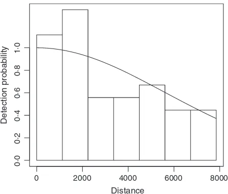
Distance sampling extends plot sampling to the case where detection is not certain. Observers move along lines or visit points and record the distance from the line or point to the object of interest (y). These distances are used to estimate the detection function,g(y) (e.g., Fig. 1), by modelling the decrease in detectability with increasing distance from the line or point

(conventional distance sampling, CDS). The detection func-tion may also include covariates (multiple covariate distance sampling, MCDS; Marqueset al.2007) that affect the scale of the detection function. From the fitted detection function, the average probability of detection can be estimated by integrat-ing out distance. The estimated average probability that an ani-mal is detected given that it is in the area covered by the survey,

^

pi, can then be used to estimate abundance as

^

N¼A a

Xn

i¼1 si

^

pi;

eqn 1

whereAis the area of the study region,ais the area covered by the survey (i.e. the sum of the areas of all of the strips/circles) and the summation takes place over thenobserved clusters, each of sizesi(if individuals are observed,si ¼ 18i) (Buck-landet al.2001, Chapter 3). Often up to half the observations in a plot sampling data set are discarded to ensure the assump-tion of certain detecassump-tion is met. In contrast, distance sampling uses observations that would have been discarded to model detection (although typically some detections are discarded beyond a giventruncation distanceduring analysis).

Estimators such as eqn 1 rely on the design of the study to ensure that abundance estimates over the whole study area (scaling up from the covered region) are valid. This article focusses onmodel-basedinference to extrapolate to a larger study area. Specifically, we consider the use of spatially explicit models to investigate the response of biological populations to *Correspondence author. E-mail: dave@ninepointeightone.net

©2013 The Authors. Methods in Ecology and Evolution©2013 British Ecological Society

biotic and abiotic covariates that vary over the study region. A spatially explicit model can explain the between-transect varia-tion (which is often a large component of the variance in design-based estimates), and so using a model-based approach can lead to smaller variance in estimates of abundance than design-based estimates. Model-based inference also enables the use of data from opportunistic surveys, for example inci-dental data arising from ‘ecotourism’ cruises (Williamset al. 2006).

Our aims in creating a spatial model of a biological popu-lation are usually twofold: (i) estimating overall abundance and (ii) investigating the relationship between abundance and environmental covariates. As with any predictions that are outside the range of the data, one should heed the usual warnings regarding extrapolation. For example, if a model contains elevation as a covariate, predictions at high, unsam-pled elevations are unlikely to be reliable. Frequently, maps of abundance or density are required and any spurious predictions can be visually assessed, as well as by plotting a histogram of the predicted values. A sensible definition of the region of interest avoids prediction outside the range of the data.

In this article, we review the current state of spatial model-ling of detection-corrected count data, illustrating some recent developments useful to applied ecologists. The methods dis-cussed have been available in Distance software (Thomaset al. 2010) for some time, but the recent advances covered here have been implemented in a newRpackage,dsm(Milleret al.2013) and are to be incorporated into Distance.

Throughout this article, a motivating data set is used to illus-trate the methods. These data are sightings of pantropical spot-ted dolphins (Stenella attenuata) during April and May of 1996 in the Gulf of Mexico. Observers aboard the NOAA vessel Oregon II recorded sightings and environmental covariates (see http://seamap.env.duke.edu/dataset/25 for survey details). A complete example analysis is provided in Appendix S1. The

data used in the analysis are available as part of thedsm pack-age and Distance.

The rest of the article reviews approaches for the spatial modelling of distance sampling data before focussing on the density surface modelling approach of Hedley & Buckland (2004) to estimate abundance and uncertainty. We then describe recent advances and provide practical advice regard-ing model fittregard-ing, formulation and checkregard-ing. Finally, we discuss future directions for research in spatially modelling detection-corrected count data.

Approaches to spatial modelling of distance sampling data

Modelling of spatially referenced distance sampling data is equivalent to modelling spatially referenced count data, with the additional information provided by collecting distances to account for imperfect detection. We review recent efforts to model such data; some consist of two steps (correction for imperfect detection, then spatial modelling), whilst others jointly estimate the relevant parameters.

T W O - S T A G E A P P R O A C H E S

The focus of this article is the ‘count model’ of Hedley & Buckland (2004); we will henceforth refer to this approach as density surface modelling(DSM). Modelling proceeds in two steps: a detection function is fitted to the distance data to obtain detection probabilities for clusters (flocks, pods, etc.) or individuals. Counts are then summarized per segment (contig-uous transect section). A generalized additive model (GAM; e.g. Wood 2006) is then constructed with the per-segment counts as the response with either counts or segment areas cor-rected for detectability (seeDensity surface modelling, below). GAMs provide a flexible class of models that include general-ized linear models (GLMs; McCullagh & Nelder 1989) but extend them with the possible addition of splines to create smooth functions of covariates, random effects terms or corre-lation structures. We cover advances using this approach in Recent developments.

As with the DSM approach, Niemi & Fernandez (2010) used a two-step procedure: first fitting a detection function, then using a Bayesian point process to model spatial pattern (fitted using MCMC). Object density was described by an intensity function, which included spatially referenced covari-ates. A possible disadvantage of their approach was that the distance function was assumed fixed once its parameters are estimated, and thus, uncertainty may not be correctly propa-gated into final abundance estimates.

Ver Hoefet al. (2013) also included separate density and detection models for seals in the Bering Sea. However, they were able to separate the detection process into three compo-nents: (i) incomplete detection on the transect line, (ii) declining detection probability as a function of distance and (iii) avail-ability bias (as seals could only be observed when hauled out on ice flows). After correcting counts for uncertain detection, they used a hierarchical, zero-inflated spatial regression model to

0 2000 4000 6000 8000

0·0

0·2

0·4

0·6

0·8

1·0

Distance

Detection probability

estimate abundance, propagating variance associated with each stage of modelling into final estimates. The analysis shows that when extra information is available (such as telemetry data for the haul-out process), additional insight can be derived.

We note that there are many approaches to modelling spa-tially referenced count data (Oppelet al. 2012, provides an overview of such methods for marine bird modelling). Also worthy of note is the approach of Barry & Welsh (2002) who used a two-stage approach to model presence/absence then spatial distribution (each via a separate GAM) to account for zero inflation.

O N E - S T A G E A P P R O A C H E S

Rather than fitting two separate models, some authors have estimated parameters of the detection and spatial models simultaneously. Perhaps the first such example was Royle et al.(2004), who considered an integrated likelihood model for point and line transects. The approach views abundance as a nuisance variable which was integrated out of the likelihood, but inferences may still be made about factors affecting under-lying density (including covariate effects). This approach was originally developed for binned distance data, but was extended by Chelgren et al. (2011) for continuous distance data.

Both Schmidtet al.(2011) and Connet al.(2012) took data augmentation approaches to add unobserved clusters within their hierarchical Bayesian models. Schmidtet al.(2011) used a presence-/absence-type model and a super-population approach (as in Royle & Dorazio 2008). Connet al.(2012) augmented observations only within the sampled transects using RJMCMC. Looking at the problem at a coarser spatial resolution (stratum-level), Moore & Barlow (2011) separated the problem into observation and process components using a state-space model. The process component described the underlying population density as it changed over time and space, which was linked to the data via the detection function.

Another point process-based approach is that of Johnson et al. (2010), who used a Poisson process to model the locations of individuals in the survey area. Unlike Niemi & Fernandez (2010), parameters of the intensity function were estimated jointly with detection function parameters via stan-dard maximum likelihood methods for point processes (Baddeley & Turner 2000) (allowing uncertainty from both the spatial pattern and detection function to be included in vari-ance estimates). A post hoc correction factor was used to address overdispersion unmodelled by spatial covariates (i.e. counts that do not follow a Poisson mean–variance relation-ship).

O N E - V S . T W O - S T A G E A P P R O A C H E S

Generally, very little information is lost by taking a two-stage approach. This is because transects are typically very narrow compared with the width of the study area so, provided no significant density variation takes place ‘across’ the width of the lines or within the point, there is no information in the

distances about the spatial distribution of animals (this is an assumption of two-stage approaches).

Two-stage approaches are effectively ‘divide and conquer’ techniques: concentrating on the detection function first, and then, given the detection function, fitting the spatial model. One-stage models are more difficult to both estimate and check as both steps occur at once; models are potentially simpler from the perspective of the user and perhaps more mathemati-cally elegant.

Two-stage models have the disadvantage that to accurately quantify model uncertainty one must appropriately combine uncertainty from the detection function and spatial models. This can be challenging; however, the alternative of ignoring uncertainty from the detection process (e.g. Niemi & Fern an-dez 2010) can produce confidence or credible intervals for abundance estimates that have coverage below the nominal level. More information regarding how variance estimation is addressed for DSMs is given inRecent developments.

Density surface modelling

This section focuses on modelling the density/abundance esti-mation stage of the DSM approach introduced previously. Both line and point transects can be used, but if lines are used, then they are split into contiguoussegments(indexed by j), which are of lengthlj. Segments should be small enough such that neither density of objects nor covariate values vary appre-ciably within a segment (making the segments approximately square is usually sufficient; 2w92w, wherewis the truncation distance). The area of each segment enters the model as (or as part of) an offset: the area of segmentjisAj ¼ 2wljand for pointjisAj ¼ pw2.

Count or estimated abundance (per segment or point) is then modelled as a sum of smooth functions of covariates (zjk withkindexing the covariates, for example location, sea sur-face temperature, weather conditions, measured at the seg-ment/point level) using a generalized additive model. Smooth functions are modelled as splines, providing flexible unidimen-sional (and higher-dimenunidimen-sional) curves (and surfaces, etc.) that describe the relationship between the covariates and response. Wood (2006) and Ruppertet al.(2003) provide more in-depth introductions to smoothing and generalized additive models.

We begin by describing a formulation where only covariates measured per-segment (e.g. habitat, Beaufort sea state) are included in the detection function. We later expand this simple formulation to include observation level covariates (e.g. cluster size, species)

CO UNT A S RESPO N SE

The model for the count per segment is:

EðnjÞ ¼p^jAjexp b0þ X

k fk zjk

" #

;

probability of detection (p^j) gives theeffective areafor segment j. If there are no covariates other than distance in the detection function, then the probability of detection is constant for all segments (i.e.p^j ¼ p,^ ∀j). The distribution ofnjcan be mod-elled as an overdispersed Poisson, negative binomial or Twee-die distribution (seeRecent developments).

Fig. 2 shows the raw observations of the dolphin data, along with the transect lines, overlaid on the depth data. A half-nor-mal detection function was fitted to the distances and is shown in Fig. 1. Figure 3 shows a DSM fitted to the dolphin data. The top panel shows predictions from a model where depth was the only covariate, and the bottom panel shows predictions where

a (bivariate) smooth of spatial location was also included. Comparing the models using GCV score, the latter had a con-siderably lower score (39.12 vs. 48.46) and so would be selected as our preferred model.

In addition to simply calculating abundance estimates, rela-tionships between covariates and abundance can be illustrated via plots of marginal smooths. The effect of depth on abun-dance (on the scale of the link function) for the dolphin data can be seen in Fig. 4.

An alternative to modelling counts is to use the per-segment/circle abundance using distance sampling estimates as the response. In this case, we replacenjby:

−200 0 200

−800 −400 0 400

Easting

Northing

Group size

200 400 600

200 1000 2000 3000

Depth (m)

Fig. 2.The region, transect centrelines and location of detected pantropical dolphin clusters, where size of circle corresponds to the cluster size, overlaid onto depth data.

−200 0 200

−500 0 500

Easting

Nor

thing

0 500 1000 1500

Abundance

−200 0 200

−500 0 500

Easting

Nor

thing

0 500 1000 1500

Abundance

^

Nj¼ XRj

r¼1 sjr

^

pj;

whereRj is the number observations in segmentjandsjr is the size of therth cluster in segmentj(if the animals occur individually, thensjr ¼ 1,∀j,r).

The following model is then fitted:

EðN^jÞ ¼Ajexp b0þ X

k fk zjk

" #

;

whereN^j, as withnj, is assumed to follow an overdispersed Poisson, negative binomial or Tweedie distribution (seeRecent developments, below). Note that the offset (Aj) is now the area of segment/point rather than effective area of the segment/ point. AlthoughN^j can always be modelled instead ofnj, it seems preferable to usenjwhen possible, as one is then model-ling actual (integer) counts as the response rather than estimates. Note that althoughN^jmay take non-integer values, this does not present an estimation problem for the response distributions covered here.

DSM with covariates at the observation level

The above models consider the case where the covariates are measured at the segment/point level. Often covariates (zij, for individual/clusteriand segment/point j) are collected on the level of observations, for example sex or cluster size of the observed object or identity of the observer. In this case, the probability of detection is a function of the object (individ-ual or cluster) level covariatesp^ðziÞ. Object level covariates can

be incorporated into the model by adopting the following estimator of the per-segment/point abundance:

^

Nj¼ XRj

r¼1 sjr

^

pðzrjÞ :

Density, rather than abundance, can be modelled by exclud-ing the offset and instead dividexclud-ing the count (or estimated abundance) by the area of the segment/point (and weighting observations by the segment/point areas). We concentrate on abundance here; see Hedley & Buckland (2004) for further details on modelling density.

P R E D ICT IO N

A DSM can be used to predict abundance over a larger/differ-ent area than was originally surveyed. In that case, the investi-gator must create a series of prediction cells over the prediction region. For each cell, the covariates included in the DSM must be available; the area of each cell is also required. Having made predictions for each cell, these can be plotted as an abundance map (as in Fig. 3) and, by summing over cells, an overall estimate of abundance can be calculated. It is worth noting that using prediction grid cells that are smaller than the resolution of the spatially referenced data has no effect on abundance/density estimates.

VARIANCE ESTIMATION

Estimating the variance of abundances calculated using a DSM is not straightforward: uncertainty from the estimated parameters of the detection function must be incorporated into the spatial model. A second consideration is that in a line transect survey, abundances in adjacent segments are likely to be correlated; failure to account for this spatial autocorrelation will lead to artificially low variance estimates and hence misleadingly narrow confidence intervals.

Hedley & Buckland (2004) describe a method of calculating the variance in the abundance estimates using a parametric bootstrap, resampling from the residuals of the fitted model. The bootstrap procedure is as follows.

Denote the fitted values for the model to be^g. Forb=1,…, B(whereBis the number of resamples required).

1. Resample (with replacement) the per-segment/point residu-als, storethe values inrb.

2. Refit the model but with the response set to^gþrb(where^g are the fitted values from the original model).

3. Take the predicted values for the new model and store them.

From the predicted values stored in the last step, the vari-ance originating in the spatial part of the model can be calcu-lated. The total variance of the abundance estimate (over the whole region of interest or subareas) can then be found by combining the variance estimate from the bootstrap procedure with the variance of the probability of detection from the detection function model using the delta method (which assumes that the two components of the variance are indepen-dent; Ver Hoef 2012).

0 500 1000 1500 2000 2500 3000 3500

−15

−10

−5

0

5

depth

Smooth of depth

The above procedure assumes that there is no correlation in space between segments, which are usually contiguous along transects. If many animals are observed in a particular seg-ment, then we might expect there to be high numbers in the adjacent segments. A moving block bootstrap (MBB; Efron & Tibshirani 1993, Section 8.6) can account for some of this spa-tial autocorrelation in the variance estimation. The segments are grouped together into overlapping blocks (so if the block size is 5, block one is segments 1,…,5, block two is segments 2, …,6, and so on). Then, at step (2) above, resamples are taken at the block level (rather than individual segments within a transect). Using MBB will account for correlation between the segments at scales smaller than the block size, inflating the vari-ances accordingly. Block size can be selected by plotting an autocorrelogram of the residuals from the DSM.

Both bootstrap procedures can also be modified to take detection function uncertainty into account. Distances are sim-ulated from the fitted detection function, and then the offset is re-calculated by fitting a detection function to the simulated distances.

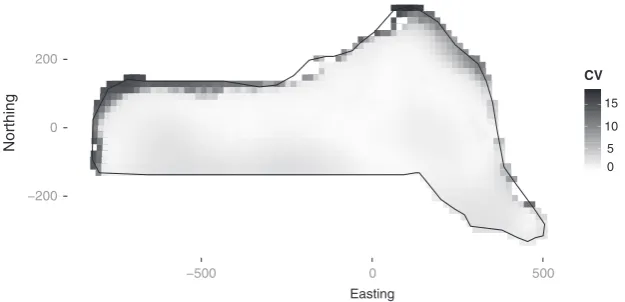
Uncertainty can be estimated for a given prediction region by calculating the appropriate quantiles of the resulting abun-dance estimates (outlier removal may be required before quan-tile calculation). DSM uncertainty can be visualized via a plot of per-cell coefficient of variation obtained by dividing the standard error for each cell by its predicted abundance (as in Fig. 5).

Recent developments

G A M UN C E R T A IN T Y A N D V A R I A N C E P R O PA G A T IO N

Rather than using a bootstrap, one can use GAM theory to construct uncertainty estimates for DSM abundance estimates. This requires that we use the distribution of the parameters in the GAM to simulate model coefficients, using them to gener-ate replicgener-ate abundance estimgener-ates (further information can found in Wood 2006, p. 245). Such an approach removes the need to refit the model many times, making variance estima-tion much faster.

Williamset al.(2011) go a step further and incorporate the uncertainty in the estimation of the detection function into the variance of the spatial model, albeit only when segment level covariates are in the DSM. Their procedure is to fit the density surface model with an additional random effect term that char-acterizes the uncertainty in the estimation of the detection function (via the derivatives of the probability of detection,p,^ with respect to their parameters). Variance estimates of the abundance calculated using standard GAM theory will include uncertainty from the estimation of the detection function. A more complete mathematical explanation of this result is given in Appendix S2.

We consider that propagating the uncertainty in this manner to be preferable to the MBB because it is more computation-ally efficient meaning investigators can easily and quickly esti-mate variances of complex models. The confidence intervals produced via variance propagation appear comparable (if not narrower) than their bootstrap equivalents, whilst maintaining good coverage (results of a small simulation study are given in Appendix S3).

Figure 5 shows a map of the coefficient of variation for the model which includes both location and depth covariates. Var-iance has been calculated using the varVar-iance propagation method.

Edge effects

Previous work (Ramsay 2002; Wang & Ranalli 2007; Wood et al.2008; Scott-Haywardet al.2013; Miller 2012) has high-lighted the need to take care when smoothing over areas with complicated boundaries, for example, those with rivers, pen-insulae or islands. If two parts of the study area (either side of a river or inlet, say) are inappropriately linked by the model (i.e. if the distance between the points is measured as a straight line, rather than taking into account obstacles), then the boundary feature (river, etc.) can be ‘smoothed across’ so positive abun-dances are predicted in areas where animals could not possibly occur. Ensuring that a realistic spatial model has been fitted to the data is essential for valid inference. The soap film smoother of Wood et al. (2008) is an appealing solution: a bivariate −200

0 200

−500 0 500

Easting

Northing

0 5 10 15

CV

smooth function of location that can be included in any GAM but that allows for boundary conditions to be estimated and obeyed for a complex study area. Such an approach can be helpful when uncertainty is estimated via a bootstrap as edge effects can also cause large, unrealistic predictions which can plague other smoothers (Bravington & Hedley 2009).

Even if the study area does not have a complicated bound-ary, edge effects can still be problematic. Miller (2012) notes that some smoothers have plane components that tend to cause the fitted surface to increase unrealistically as predictions are made further away from the locations of survey effort. This problem can be alleviated using a different type of smoother (e.g. a generalization of thin plate regression splines called Duchon splines).

Tweedie distribution

The Tweedie distribution offers a flexible alternative to the quasi-Poisson and negative binomial distributions as a response distribution when modelling count data (Candy 2004). In particular, it is useful when there are a high propor-tion of zeros in the data (Shono 2008; Peelet al.2012) and avoids multiple-stage modelling of zero-inflated data (as in Barry & Welsh 2002).

The distribution has three parameters: a mean, dispersion and a third power parameter, which leads to additional flexibil-ity. The distribution does not change appreciably when the power parameter is changed by less than 0.1, and therefore, a simple line search over the possible values for the power parameter is usually a reasonable approach to estimating the parameter. M. Bravington (pers. comm.) suggested plotting the square root of the absolute value of the residuals against fit-ted values; a ‘flatter’ plot (points forming a horizontal line) gives an indication of a ‘good’ value. We additionally suggest using the metrics described in the next section for model selection.

Appendix S4 gives further details about the Tweedie distri-bution (including its probability density function and further references).

Practical advice

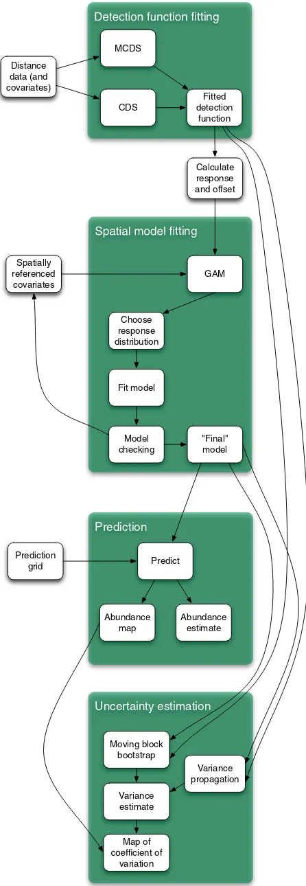
A flow diagram of the modelling process for creating a DSM is shown in Fig. 6. The diagram shows which methods are com-patible with each other and what the options are for modelling a particular data set.

In our experience, it is sensible to obtain a detection func-tion that fits the data as well as possible and only begin spa-tial modelling after a satisfactory detection function has been obtained. Model selection for the detection function can be performed using AIC and model checking using goodness-of-fit tests given in the study by Burnham et al. (2004) Section 11.11). If animals occur in clusters rather than indi-vidually, bias can be incurred due to the higher visibility of larger clusters. It may then be necessary to include size as a covariate in the detection function (see Bucklandet al.2001, Section 4.8.2.4). For some species, cluster size may change Calculate

response and offset

tting

Spatially referenced covariates

GAM

Choose response distribution

Fit model

Model checking

"Final" model Distance

data (and covariates)

tting

MCDS

CDS

Fitted detection

function

Uncertainty estimation

Variance propagation

Variance estimate

Map of cient of variation Moving block

bootstrap

Prediction

Predict

Abundance map

Abundance estimate Prediction

grid

according to location; Fergusonet al.(2006) use two GAMs (one to model observed clusters and one to model the cluster size) to deal with spatially varying cluster size amongst del-phinids, although the authors do not present the variance of the resulting predictions.

Smooth terms can be selected using (approximate)p-values (Wood 2006, Section 4.8.5). An additional useful technique for covariate selection is to use an extra penalty for each term in the GAM allowing smooth terms to be removed from the model during fitting (illustrated in Appendix S1; Wood 2011). Smoothness selection is performed by generalized cross-valida-tion (GCV) score, unbiased risk estimator (UBRE) or restricted maximum likelihood (REML) score. When model covariates are effectively functions of one another (e.g. depth could be written as a function of location), GCV and UBRE can suffer from optimization problems (Wood 2006, Section 4.5.3), which can lead to unstable models (Wood 2011). REML provides a fitting criteria with a more pronounced optima which avoids some problems with parameter estima-tion, although caution should always be taken when dealing with highly correlated covariates. A significant drawback of REML is that scores cannot be used to compare models with different linear terms or offsets (Wood 2011), although the p-value and additional penalty techniques described above can be used to select model terms. We highly recommend the use of standard GAM diagnostic plots; Wood (2006) provides further practical information on GAM model selection and fitting.

In the analysis of the dolphin data, we included a smooth of location that nearly doubles the percentage deviance explained (27.3–52.7%). One can see this when comparing the two plots in Fig. 3 and the plot of the depth (Fig. 2), the plot of the model containing only a smooth of depth looks very similar to the raw plot of the depth data. Using a smooth of location can be a primitive way to account for spatial autocorrelation and/or as a proxy for other spatially varying covariates that are unavailable.

A more sophisticated way to account for spatial autocor-relation between segments (within transects) is to use an autocorrelation structure within the DSM (e.g. autoregres-sive models). Appendix S1 shows an example using general-ized additive mixed model (GAMMs; Wood 2006, Section 6.6, see Appendix S1 for an example) to construct an autore-gressive (lag 1) correlation structure.

In the analysis presented here, spatial location has been transformed from latitude and longitude to kilometres north and east of the centre of the survey region at

ð27:01;88:3Þ. This is because the bivariate smoother used (the thin plate spline; Wood 2003) is isotropic: there is only one parameter controlling the smoothness in both directions. Moving one degree in latitude is not the same as moving one degree in longitude, and so using kilometres from the centre of the study region makes the covariates isotropic. Using metric units rather than non-standard units of measure such as degrees or feet throughout makes analysis much easier.

A smooth of an environment-level covariate such as depth can be very useful for assessing the relationships between abun-dance and the covariate (as in Fig. 4). Caution should be employed when interpreting smooth relationships and abun-dance estimates, especially if there are gaps over the range of covariate values. Large counts may occur at large values of depth, but if no further observations occur at such a large value, then investigators should be sceptical of any relation-ship.

Discussion

The use of model-based inference for determining abundance and spatial distribution from distance sampling data presents new opportunities in the field of population assessment. Spa-tial models can be particularly useful when it comes to pre-diction: making predictions for some subset of the study area relies on stratification in design-based methods and as such can be rather limited. Our models also allow inference from a sample of sightings to a population in a study area without depending upon a random sample design, and therefore, data collected from ’platforms of opportunity’ (Williams et al. 2006) can be used (although a well-designed survey is always preferable).

Unbiased estimates are dependent upon either (i) distribu-tion of sampling effort being random throughout the study area (for design-based inference) or (ii) model correctness (for model-based inference). It is easier to have confidence in the former rather than in the latter because our models are always wrong. Nevertheless, model-based inference will play an increasing role in population assessment as the availability of spatially referenced data increases.

The field is quickly evolving to allow modelling of more complex data building on the basic ideas of density surface modelling. We expect to see large advances in temporal infer-ences and the handling of zero-inflated data and spatial corre-lation. These should become more mainstream as modern spatio-temporal modelling techniques are adopted. Petersen et al. (2011) provided a very basic framework for temporal modelling; their model included ‘before’ and ‘after’ smooth terms to quantify the impact of the construction of an offshore windfarm. Zero inflation in count data may be problematic, and two-stage approaches such as Barry & Welsh (2002) as well as more flexible response distributions made possible by Rigby & Stasinopoulos (2005) have yet to be exploited by those using distance sampling data. Spatial autocorrelation can be accounted for via approaches that explicitly introduce correla-tions such as generalized estimating equacorrela-tions (GEEs; Hardin & Hilbe 2003) or generalized additive mixed models or via mechanisms such as that of Skaug (2006), which allow obser-vations to cluster according to one of several states (such as high vs low density patches, possibly in response to temporary agglomerations of prey, although the mechanism is unimpor-tant). These advances should assist both modellers and wildlife managers to make optimal conservation decisions.

computation-ally feasible (as INLA is an alternative to MCMC). An impor-tant step towards such models will be incorporation of detec-tion funcdetec-tion estimadetec-tion into the spatial model. We anticipate that such a direct modelling technique will dominate future developments in the field.

Density surface modelling allows wildlife managers to make best use of the available spatial data to understand patterns of abundance and hence make better conservation decisions (e.g. about reserve or development placement). The recent advances mentioned here increase the reliability of the outputs from a modelling exercise and hence the ‘efficacy of these decisions. Density surface modelling from survey data is an active area of research, and we look forward to further improvements and extensions in the near future.

Acknowledgements

We wish to thank Paul Conn, another anonymous reviewer and the associate editor for their helpful comments. DLM wishes to thank Mark Bravington and Sharon Hedley for their detailed discussions and for providing code for their variance propagation method. Funding for the implementation of the recent advances into thedsmpackage and Distance software came from the US Navy, Chief of Naval Operations (Code N45), Grant Number N00244-10-1-0057.

References

Baddeley, A. & Turner, R. (2000) Practical maximum pseudolikelihood for spa-tial point patterns. Australian & New Zealand Journal of Statistics, 42, 283–322.

Barry, S.C. & Welsh, A.H. (2002) Generalized additive modelling and zero inflated count data.Ecological Modelling,157, 179–188.

Bravington, M.V. & Hedley, S.L. (2009) Antarctic minke whale abundance esti-mates from the second and third circumpolar IDCR/SOWER surveys using the SPLINTR model. Paper SC/61/IA14, IWC Scientific Committee. Buckland, S.T., Anderson, D.R., Burnham, K.P., Laake, J.L., Borchers, D.L. &

Thomas, L. (2001)Introduction to Distance Sampling. Oxford University Press, Oxford, UK.

Buckland, S.T., Anderson, D.R., Burnham, K.P., Laake, J.L., Borchers, D.L. & Thomas, L. (2004)Advanced Distance Sampling. Oxford University Press, Oxford, UK.

Burnham, K.P., Buckland, S.T., Laake, J.L., Borchers, D.L., Marques, T.A., Bishop, J.R. & Thomas, L. (2004) Further topics in distance sampling.

Advanced Distance Sampling(eds. S.T. Buckland, D.R. anderson, K.P. Burn-ham, J.L. Laake, D.L. Borchers & L. Thomas), pp. 307–392. Oxford Univer-sity Press, Oxford, UK.

Candy, S. (2004) Modelling catch and effort data using generalised linear models, the Tweedie distribution, random vessel effects and random stratum-by-year effects.CCAMLR Science,11, 59–80.

Chelgren, N.D., Samora, B., Adams, M.J. & McCreary, B. (2011) Using spatio-temporal models and distance sampling to map the space use and abundance of newly metamorphosed western toads (Anaxyrus boreas).Herpetological Conservation and Biology,6, 175–190.

Conn, P.B., Laake, J.L. & Johnson, D.S. (2012) A hierarchical modeling frame-work for multiple observer transect surveys.PLoS ONE,7, e42294. Efron, B. & Tibshirani, R.J. (1993)An Introduction to the Bootstrap. Chapman &

Hall/CRC, Boca Raton, FL, USA. ISBN 9780412042317.

Ferguson, M.C., Barlow, J., Fiedler, P., Reilly, S.B. & Gerrodette, T. (2006) Spatial models of delphinid (family Delphinidae) encounter rate and group size in the eastern tropical Pacific Ocean.Ecological Modelling,193, 645– 662.

Halpin, P., Read, A., Fujioka, E., Best, B., Donnelly, B., Hazen, L., (2009) OBIS-SEAMAP: The world data center for marine mammal, sea bird, and sea turtle distributions.Oceanography,22, 104–115.

Hardin, J. & Hilbe, J. (2003)Generalized Estimating Equations. Chapman and Hall/CRC, London, UK.

Hedley, S.L. & Buckland, S.T. (2004) Spatial models for line transect sampling.

Journal of Agricultural, Biological, and Environmental Statistics,9, 181–199.

Johnson, D.S., Laake, J.L. & Ver Hoef, J.M. (2010) A model-based approach for making ecological inference from distance sampling data.Biometrics,66, 310–318.

Marques, T.A., Thomas, L., Fancy, S. & Buckland, S.T. (2007) Improving estimates of bird density using multiple-covariate distance sampling.The Auk,

124, 1229–1243.

McCullagh, P. & Nelder, J.A. (1989)Generalized Linear Models. Chapman & Hall/CRC, Boca Raton, FL, USA.

Miller, D.L. (2012)On smooth models for complex domains and distances. Ph.D. thesis, University of Bath.

Miller, D.L., Rexstad, E.A., Burt, M.L., Bravington, M.V. & Hedley, S.L. (2013)

dsm: Density surface modelling of distance sampling data. URL http:// github.com/dill/dsm

Moore, J.E. & Barlow, J. (2011) Bayesian state-space model of fin whale abun-dance trends from a 1991–2008 time series of line-transect surveys in the Cali-fornia Current.Journal of Applied Ecology,48, 1195–1205.

Niemi, A. & Fernandez, C. (2010) Bayesian spatial point process modeling of line transect data.Journal of Agricultural, Biological, and Environmental Statistics,

15, 327–345.

Oppel, S., Meirinho, A., Ramı´rez, I., Gardner, B., O’Connell, A., Miller, P. & Louzao, M. (2012) Comparison of five modelling techniques to predict the spatial distribution and abundance of seabirds.Biological Conservation,156, 94–104.

Peel, D., Bravington, M.V., Kelly, N., Wood, S.N. & Knuckey, I. (2012) A Mod-el-Based Approach to Designing a Fishery-Independent Survey.Journal of Agricultural, Biological, and Environmental Statistics,18, 1–21.

Petersen, I.K., MacKenzie, M.L., Rexstad, E.A., Wisz, M.S. & Fox, A.D. (2011) Comparing pre- and post-construction distributions of long-tailed ducks Clan-gula hyemalisin and around the Nysted offshore wind farm, Denmark: a quasi designed experiment accounting for imperfect detection, local surface features and autocorrelation. Technical report 2011–1, Centre for Research into Enivi-ronmental and Ecological Modelling.

Ramsay, T. (2002) Spline smoothing over difficult regions.Journal of the Royal Statistical Society. Series B, Statistical Methodology,64, 307–319.

Rigby, R. & Stasinopoulos, D. (2005) Generalized additive models for location, scale and shape.Journal of the Royal Statistical Society-Series C Applied Statis-tics,54, 507–554.

Royle, J.A. & Dorazio, R.M. (2008)Hierarchical Modeling and Inference in Ecol-ogy. Academic Press, London, UK.

Royle, J., Dawson, D. & Bates, S. (2004) Modeling abundance effects in distance sampling.Ecology,85, 1591–1597.

Rue, H., Martino, S. & Chopin, N. (2009) Approximate Bayesian inference for latent Gaussian models by using integrated nested Laplace approximations.

Journal of the Royal Statistical Society: Series B, Statistical Methodology,71, 319–392.

Ruppert, D., Wand, M. & Carroll, R.J. (2003)Semiparametric Regression. Cam-bridge Series on Statistical and Probabilistic Mathematics. CamCam-bridge Univer-sity Press, Cambridge, UK.

Schmidt, J.H., Rattenbury, K.L., Lawler, J.P. & Maccluskie, M.C. (2011) Using distance sampling and hierarchical models to improve estimates of Dall’s sheep abundance.The Journal of Wildlife Management,76, 317–327.

Scott-Hayward, L.A.S., MacKenzie, M.L., Donovan, C.R., Walker, C.G. & Ashe, E. (2013) Complex region spatial smoother (CReSS).Journal of Compu-tational and Graphical Statistics, doi:10.1080/10618600.2012.762920 Shono, H. (2008) Application of the Tweedie distribution to zero-catch data in

CPUE analysis.Fisheries Research,93, 154–162.

Skaug, H.J. (2006) Markov modulated Poisson processes for clustered line tran-sect data.Environmental and Ecological Statistics,13, 199–211.

Thomas, L., Buckland, S.T., Rexstad, E.A., Laake, J.L., Strindberg, S., Hedley, S.L., Bishop, J.R., Marques, T.A. & Burnham, K.P. (2010) Distance software: design and analysis of distance sampling surveys for estimating population size.Journal of Applied Ecology,47, 5–14.

Ver Hoef, J.M. (2012) Who invented the delta method?The American Statistician, 66,124–127.

Ver Hoef, J.M., Cameron, M.F., Boveng, P.L., London, J.M. & Moreland, E.E. (2013) A spatial hierarchical model for abundance of three ice-associated seal species in the eastern Bering Sea.Statistical Methodology, http://dx.doi.org/10. 1016/j.stamet.2013.03.001

Wang, H. & Ranalli, M. (2007) Low-rank smoothing splines on complicated domains.Biometrics,63, 209–217.

Williams, R., Hedley, S.L. & Hammond, P. (2006) Modeling distribution and abundance of Antarctic baleen whales using ships of opportunity.Ecology and Society,11, 1.

Wood, S.N. (2003) Thin plate regression splines.Journal of the Royal Statistical Society. Series B, Statistical Methodology,65, 95–114.

Wood, S.N. (2006)Generalized Additive Models: An introduction with R. Chap-man & Hall/CRC, Boca Raton, FL, USA.

Wood, S.N. (2011) Fast stable restricted maximum likelihood and marginal likeli-hood estimation of semiparametric generalized linear models.Journal of the Royal Statistical Society, Series B, Statistical Methodology,73, 3–36. Wood, S.N., Bravington, M.V. & Hedley, S.L. (2008) Soap film smoothing.

Journal of the Royal Statistical Society, Series B, Statistical Methodology,70, 931–955.

Received 13 March 2013; accepted 19 July 2013 Handling Editor: Olivier Gimenez

Supporting Information

Additional Supporting Information may be found in the online version of this article.

Appendix S1.Example_DSMAnalysis.

Appendix S2.Calculation of Variance in Density Surface Models.

Appendix S3.Relative Performance of Gam and Bootstrap Uncer-tainty Estimation in DSM.