1
Alireza Hajipour1, Arash Mirabdolah Lavasani1, Mohammad Eftekhari Yazdi1, Amir Mosavi2,3, Shahaboddin Shamshirband4,5*, Kwok-Wing Chau6
1Department of Mechanical Engineering, Central Tehran Branch, Islamic Azad University, Tehran, Iran (email:
[email protected], [email protected]) [email protected])
2Institute of Structural Mechanics, Bauhaus University Weimar, 99423 Weimar, Germany; [email protected] 3Institute of Automation, Kalman Kando Faculty of Electrical Engineering, Obuda University, 1034 Budapest,
Hungary
4Department for Management of Science and Technology Development, Ton Duc Thang University, Ho Chi Minh
City, Vietnam
5Faculty of Information Technology, Ton Duc Thang University, Ho Chi Minh City, Vietnam
6Department of Civil and Environmental Engineering, Hong Kong Polytechnic University, Hung Hom, Hong Kong,
China; (email: [email protected])
*Corresponding author, Email: [email protected]
Abstract
In the present paper, an aerodynamic investigation of a high-speed train is performed. In the first
section of this article, a generic high-speed train against a turbulent flow is simulated,
numerically. The Reynolds-Averaged Navier-Stokes (RANS) equations combined with the 𝑘-𝜔
SST turbulence model are applied to solve incompressible turbulent flow around a high-speed
train. Flow structure, velocity and pressure contours and streamlines at some typical wind
directions of θ = 0˚, 30˚, 45˚ and 60, are the most important results of this simulation. The
maximum and minimum values are specified and discussed. Also, the pressure coefficient for
some critical points on the train surface is evaluated. In the following, the wind direction
influence the aerodynamic key parameters as drag, lift, and side forces at the mentioned wind
directions are analyzed and compared. Moreover, the effects of velocity changes (50, 60, 70, 80
and 90 m/s) are estimated and compared on the above flow and aerodynamic parameters. In the
2
second section of the paper, various data-driven methods including Gene Expression
Programming (GEP), Gaussian Process Regression (GPR), and random forest (RF), are applied
for predicting output parameters. So, drag, lift and side forces and also minimum and maximum
of pressure coefficients for mentioned wind directions (θ = 0° to θ = 60°) and velocity (50 m/s to
90 m/s) are predicted and compared using statistical parameters. Obtained results indicated that
RF in all coefficients of wind direction and most coefficients of free stream velocity provided the
most accurate predictions. As a conclusion, RF may be recommended for the prediction of
aerodynamic coefficients.
Keywords: High-speed train; prediction, turbulence model; hybrid machine learning;
aerodynamics
1.
Introduction
The research on the flow around high-speed trains is considered a popular subject among
engineering applications. Many countries have built high-speed train lines to link cities,
including Germany, China, Austria, Belgium, France, Poland, Italy, Portugal, Japan, Russia,
South Korea, Spain, Sweden, Taiwan, Turkey, United Kingdom, United States and etc.
Nowadays, trains move at high speed, study of the aerodynamic characteristics of the air flow
around them is an interesting topic. In recent years, many simulations of flow over high-speed
trains have been performed. The most significand and related of them reviewed in previous
3
number (almost 109) was used for aerodynamic analysis.
Effect of cross-wind on a high-speed train was investigated, numerically (Khier, 2002). In
this paper, the flow over the German InterRegio high-speed train were simulated using
Reynolds-averaged Navier-Stokes and k-ε turbulence model.
Effects of crosswind on the German InterRegio high-speed train was estimated (Fauchier,
2002). For the numerical simulation, the RANS approach along with RNG k-ε turbulent model
was implemented. In this analysis, at first, a preliminary study has been done on a simple
geometry of train via CFD. Then, a three-dimensional model of the train in three following cases
have been investigated.
A research of aerodynamic flow characteristics on a high speed train was done (Shin, 2003).
In this numerical study, the variation of in the aerodynamic forces were performed for the high
speed train at the entrance of a tunnel.
A numerically investigation of the fluid flow around a high-speed train was done (Tian,
2009). As the high speed at modern train is effective in aerodynamic drag, reducing drag and
consequently reducing energy consumption is one of the main issues in the development of the
rail industry.
An aerodynamic characteristic of a Chinese high-speed train using RANS numerical method
was performed (Zhao, 2009). In this research, the aerodynamic influences were studied with the
train at the entrance and exit of a tunnel.
An optimization of aerodynamic characteristics of high-speed train using numerical method
4
response surfaces instead of complex NS simulations and Genetic Algorithm (GA) an
optimization aerodynamic properties have been conducted on Swedish high-speed train X2000.
A simulation of a high-speed train at a tunnel entrance was presented (Li, 2011). For this
purpose, the RANS numerical method and k-ε turbulent model for a viscous compressible fluid
was applied.
A numerical simulation of EMU high-speed train using RANS method and RNG k-ε
turbulent model was conducted (Wang, 2012). The main reason for this research was the
pressure changes and aerodynamic forces with two trains passing alongside each other in a
tunnel.
A numerical aerodynamic characteristics of a high-speed train against a crosswind using
unsteady three dimensional RANS approach and k-ε turbulent model was done (Asress, 2014). In
the simulation, two scenarios for ground as static and moving for yaw angles ranges from 30˚ to
60˚ were considered.
A numerical simulation about wind effect on a high-speed train was done (Peng, 2014). A
three dimensional incompressible RANS method and k-ε turbulent model has been done For
simulation of air flow passing a simple high-speed train.
An optimization of aerodynamic parameters for high-speed trains was investigated useing
numerical method (Shuanbao, 2014). The complicated wake flow deeply affects the movement
of the trains.
An aerodynamic simulation of two high-speed trains in a tunnel using RANS numerical
method and RNG k–ε turbulence model (Chu, 2014). In this paper, a three-dimensional,
5
most important goals of this article to determine. Also, the surface pressure and aerodynamic
forces of train were analyzed using RANS approach combined with the eddy viscosity
hypothesis in turbulence model.
A comparison between Reynolds-averaged Navier–Stokes (RANS) turbulence models and
experimental wind tunnel findings by Detached Eddy Simulation (DES) for pressure on a
high-speed train was conducted (Morden, 2015). The k-ε, k-ε re-normalization group (RNG),
realizable k-ε, Spalart–Allmaras (S-A) and shear stress transport (SST k-ω) are the five
numerical models of RANS used in this article.
An aerodynamic investigation on a simple model of high-speed train under crosswind using
the numerical method of large eddy simulation (LES) was performed (Zhuang, 2015). In this
study, the effects of flow diversion were investigated with two angles of φ = 30˚ and 60˚ using
LES.
A CFD simulation using RANS numerical method for a high-speed train against a crosswind
for two conditions; stationary and moving was conducted (Catanzaro, 2016). The effect of each
conditions was analyzed.
An aerodynamic design on a high-speed train was done (Ding, 2016). Due to the speed
improvements of the high-speed trains and increasing the aerodynamic effect of the mechanical
one, the effects and issues of aerodynamics were considered as the main challenge of this paper.
An aerodynamic performance of a train under crosswinds condition using RANS numerical
method was investigated (Liu, 2016). In this research, via the computational fluid dynamics, the
6
An aerodynamic comparison between two trains, a static and a moving was done (Premoli,
2016). In this research, using the numerical RANS method the simulation results of the relative
movements of the trains between the vehicle and its infrastructure that was effective on the
aerodynamic coefficients were compared.
In the present study, the key flow parameters such as pressure, velocity and the aerodynamic
parameters of a turbulent air flow around a generic high-speed train are analyzed. Moreover, the
mentioned parameters are predicted by the data driven methods of GEP, GPR and RF. Then,
using evaluation parameters, the most accurate model is suggested.
2.
Computational Simulation
2.1. Geometry Description
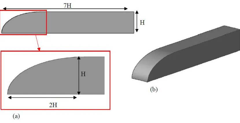
The train model used in present paper is a generic high-speed train one which has been used
in many research studies on high-speed trains. Figure 1 shows that the geometry of the generic
high-speed train model with different views. The geometric characteristics of the train are as
follows:
As Figure 1, the nose form of the train is elliptical. Also, the length, height and width of the
7
Figure 1. Geometry of the generic high-speed train; (a): Side view, (b): Isometric view.
2.2. Domain Description
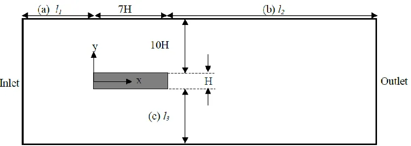
The train model is placed 0.15H above the ground. The length, width, and height of the
computing domain are 36H × 21H × 11.15H, respectively. The distance between then inlet of the
domain and the nose of the train and between the outlet of the domain and the back of the train
are 8H and 21H, respectively. Moreover, the distance between train and two sides of the domain
is 10H (see Figures 2-4).
8
Figure 3. Front view of the computational domain.
Figure 4. Top view of the computational domain.
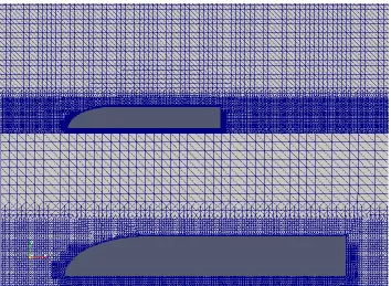
2.3. Mesh Description
The used mesh in the computational domain for the different cases (wind directions of θ = 0˚,
30˚, 45˚ and 60˚) are 4,000,000 nodes, approximately and the y+ range are between 73.2 and
94.3. For these cases, the y+ must be located between 30 to 300. In the following, two refinement
9
Figure 5. Wide and close view of the two refinement boxes near and around the train.
2.4. Boundary Conditions
The defined boundary conditions of the case are as follows:
Inlet: a uniform velocity, that represents the free stream velocity, U∞ in the x direction.
Outlet: the patch type boundary condition with a free stream value.
Sides and top of the domain: the patch type boundary condition with a free stream value.
Ground: The wall boundary condition used for the ground.
Train surface: The wall boundary condition used for the train.
Also, the Reynolds number, Re, according to the height of the train, H = 0.56 m, free stream
velocity, U∞= 70 m/s, and kinematic viscosity, ν = 1.5 × 10⁻⁵, (Re = U∞× H/ ν) is 2.6 × 10⁶.
10
The air flow field around the high-speed train which defined as a 3D incompressible
turbulent flow is solved by the Reynolds-Averaged Navier-Stokes (RANS) equation combined
with the 𝑘-𝜔 Shear-Stress Transport (SST) turbulence approach. The Reynolds-Averaged
Navier-Stokes, is a time-average method of fluid flow description. In this method, instantaneous
quantities are replaced by average and oscillating ones.
According to the selected solution method, The continuity and Navier-Stokes equations for
the incompressible air flow around the train as follows:
where, i, j and k = 1, 2 and 3 are related to the streamwise –x, cross-stream –y and –z
direction, respectively. The velocity ingredients, and the pressure, are both nonlinear terms.
Hence, there aren’t any analytical solves for the problem with optional boundary conditions. The
transience of the flow parameters (i.e. velocity and pressure) are divided into mean value and
fluctuations as follows:
where and are the time-averaged, while and are the fluctuation terms of velocity
and pressure, respectively. Substituting the Reynolds divided velocities and pressures into the
Continuity and Navier-Stokes equations yields the RANS equation of motions as illustrated
11
According to the Boussinesq, the Reynolds-stress tensor could be connected to the mean rate
of deformation. The concept applied for the turbulence model is as below:
where, the turbulent kinetic energy (𝑘) and the specific dissipation rate (𝜔) are solved via the
following equations:
Turbulence Kinetic Energy, 𝑘
Specific Dissipation Rate, 𝜔
where, 𝜈𝑇 is the kinematic eddy viscosity which defined as follows:
The following closure coefficient is applied in the paper:
12
3.
Aerodynamic Results and Discussions
3.1. Flow Structure
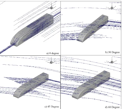
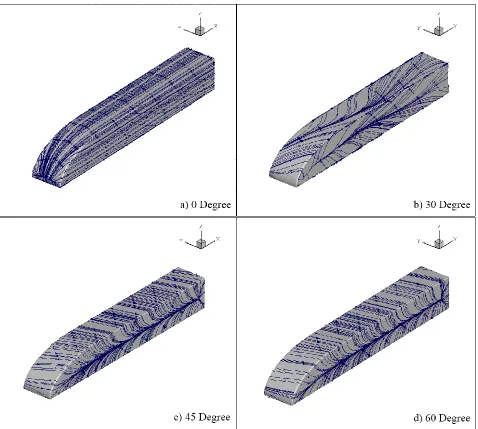
It is clear that the wind direction has significant influence on the flow structure around the
generic high-speed train. In this section, the influence of free stream direction at four different
angles of wind directions of θ = 0˚, 30˚, 45˚ and 60˚ perpendicular to the x-axis with constant
velocity magnitude is presented graphically in Figure 6. It should be noted that the obtained flow
13
Figure 6. Three-dimensional time-averaged flow structures for different wind direction angles.
As it can be seen in Figure 10, the circulations at the lee-side of the generic train model were
created. These circulations at each section along the length of model are consists of two main
circulations which are kindled form roof-side and bottom-side of the model. Furthermore, the
length and width of the circulations changes along the length of model. It is obvious in the
figures that the nose of the model has considerable influence on the three-dimensional flow
14
should be noted that the circulation existing at the leeward of the model enhances the pressure
coefficient and resulted drag force.
In order to comprehensive investigation of the flow structure, the flow pattern at two most
important regions were investigated for windside and leeward. The leeward flow patterns are
identified by three-dimensional and two dimensional flow patterns. Since the three-dimensional
flow structures at the windside will not render clear insight, the stream lines at the surface of the
generic train model are obtained in Figure 7. It can be observed that the positions of the
stagnation lines at the surface of model’s body are almost similar for all cases. On the other
hand, the stagnation lines at the model’s nose are deflected to roofward of the model. It is due to
the fact that the air flow is imposed to be passed form roofward due to limited space at the
bottom of the train model. Totally, the variation of wind direction has no pronounced influence
on the flow pattern at the windside region.
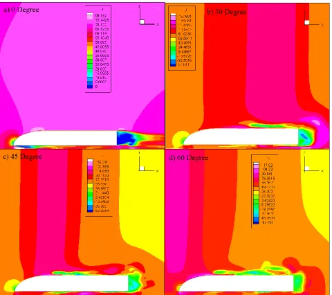
The two-dimensional total pressure contours over the train for different wind directions (θ =
0˚, 30˚, 45˚ and 60˚) are presented in Figure 8. The pressure distribution around the train are the
same for the different wind directions, generally. The pressure at the front and the back of the
15
16
Figure 8. Two dimensional pressure distribution around the train for different wind direction angles.
Moreover, the two dimensional velocity distribution (x-axis velocity: U) around the train for
different wind direction angles are illustrated in Figure 9. Based on principles, the velocity value
17
18
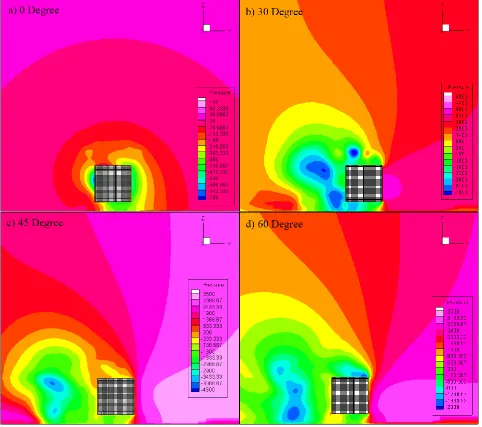
Figure 10. Two dimensional pressure distribution along train cross section for different wind direction angles.
Also, Figure 10 shows the two dimensional pressure distribution along train cross section for
different wind direction angles (θ = 0˚, 30˚, 45˚ and 60˚). All cases illustrate the low region of
pressure at the leeside of the train if compared to the windward side.
19
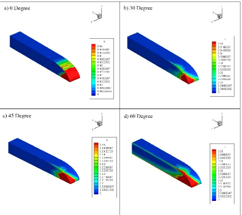
12, respectively. As the air stream collides with the generic train model, the regime of air flow
stream changes form laminar to turbulent. The zones with turbulent regime and the intensity of
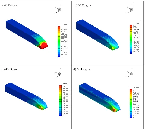
turbulence may be identified with kinetic turbulent energy parameter. As shown as Figure 13, in
case of θ = 0°, the highest value of turbulent kinetic energy occurs at the adjacent of the nose of
the model. Furthermore, the turbulent kinetic energy reduces level by level as the air flow getting
away from the generic train model. It is due to the fact that the air flow speed becomes slower
and the disordered flow structure changes to regular flow pattern. In addition, it is clear that the
nose of the model has pronounced influence on determining the turbulent region. In the next
cases with θ = 30°, 45° and 60°, the regions with different turbulent kinetic energy are totally
irregular as same as the three-dimensional flow structure at this case. It can be observed that the
regions near to the train model have higher value of turbulent kinetic energy.
The specific turbulence dissipation is the rate at which turbulence kinetic energy is converted
into thermal internal energy per unit volume and time. The values of specific turbulent
dissipation rate for the cases θ = 0°, 30°, 45° and 60° are almost similar with each other. The
contours of specific dissipation rate reveal that the maximum value of this parameter occurs at
20
21
Figure 12. Surface Specific Dissipation Rate for different wind direction angles.
3.3. Aerodynamic Forces
The most significant and practical aerodynamic parameters for bluff bodies simulation are
lift, drag and side forces. To achieve this, the mentioned forces for train case for different wind
directions are defined and estimated, clearly. The lift force and the drag force coefficients are
22
and
where, and are the drag and lift forces, and are the surface area of the train in y-
and z- directions, respectively. Moreover, the side force coefficient is defined as follows:
where, and are the side force and the side surface area of the train in x- direction,
respectively. Also, the pressure coefficient is as follow:
where, , and are the free stream pressure, density and free stream velocity,
respectively.
For verifying the extracted data from this paper, did an approximate comparison between the
aerodynamic coefficients obtained from this paper and the (Zhuang, 2015). The geometric
conditions of the two papers are as the same and for more accuracy the free stream velocity was
considered U∞= 20 m/s, as the (Zhuang, 2015). The comparison results is illustrated as Table 1.
The comparison show that the a good agreement between the results of this paper and the
obtained results from (Zhuang, 2015).
In the following, for different wind directions of this research, i.e. 0˚, 30˚, 45˚ and 60˚ and for
23
train movement increase too. Moreover, in Table 3, the time-averaged of the minimum,
maximum and average values of the pressure coefficients for mentioned different wind directions
are listed and compared. As the same way, with increasing the wind direction of the free stream,
the numerical values of the minimum, maximum and the average values of the pressure
coefficients increase too. Also, the maximum value of pressure coefficient at 60˚ wind direction
has the highest value.
Then, the exact pressure coefficient for different nodes on the train surface as Figure 13 are
shown in Figure 14. As shown in Figure 14, the top nodes of the train roof which are the
midpoints of the roof to pressure coefficients analysis and compare are considered. The desired
values are listed in Figure 14 based on the marked points.
Table 1. Comparison of time-averaged values of the lift and side forces between the paper and the (Zhuang, 2015). Cases
Wind directions
This paper (Zhuang, 2015)
CL CS CL CS
θ = 30° 0.90 0.71 0.136 0.424
θ = 60° 1.63 1.42 0.161 1.029
Table 2. Time-average aerodynamic force coefficients for different wind directions.
Aerodynamic Coeffs. , Lift Coefficient , Drag Coefficient , Side Coefficient
0° 0.34 0.48 0.01
24
45° 1.06 0.92 2.61
60° 1.63 1.42 3.02
Table 3. Time-average minimum, maximum and average pressure coefficients for different wind directions.
Pressure Coeffs.
0° -1.91 0.98 -0.10
30° -4.10 2.88 -0.03
45° -6.72 4.56 -0.40
60° -7.80 4.66 -0.33
25
1 2 3 4 5 6 7 8 9 10 11
0 0.05 0.1 0.15 0.2 0.25 0.3
Different nodes on the train surface
-C P , P re ss u re C o ef fi ci en t
Figure 14. Pressure coefficients for different nodes on the train surface.
In this part, two comparisons on some aerodynamic key parameters for five different free
stream velocity as 50, 60, 70, 80 and 90 m/s (and consequently five different Reynolds numbers
as 1.9×10⁶, 2.2×10⁶, 2.6×10⁶, 3.0×10⁶ and 3.4×10⁶) are done.
In the following, for the different free stream velocity, the lift, drag and side aerodynamic
coefficients are compared which are illustrated in Table 4. As it can be seen from Table 4, when
the wind velocity increases, the lift, drag and side aerodynamic coefficients increase. Then, the
friction and resistance against train movement increase too.
Moreover, in Table 5, the time-averaged of the minimum, maximum and average values of
the pressure coefficients for the different wind velocity and Reynolds numbers are listed and
compared. According to the results, the maximum value of the pressure coefficient is related to
the 90 m/s velocity.
In the following, the aerodynamic drag coefficient for some points during the train length is
26
aerodynamic drag for 15 points during the train length for 5 air flow velocity (50, 60, 70, 80 and
90 m/s) is analyzed. With increasing the air flow velocity, the aerodynamic drag for similar
points increase too. Also, from the nose to the end of the train, the aerodynamic drag has a
downward trend. Moreover, The maximum value of the drag coefficient is related to the case of
90 m/s and occurs at the nose of the train.
Table 4. Time-average aerodynamic force coefficients for different free stream velocity.
Aerodynamic Coeffs. , Lift Coefficient , Drag Coefficient , Side Coefficient
50 (m/s) 0.23 0.36 0.012
60 (m/s) 0.29 0.41 0.019
70 (m/s) 0.36 0.48 0.018
80 (m/s)
90 (m/s)
0.46
0.53
0.53
0.69
0.024
0.027
Table 5. Time-average minimum, maximum and average pressure coefficient for different free stream velocity. Pressure Coeffs.
50 (m/s) -0.97 0.50 -0.05
60 (m/s) -1.40 0.72 -0.06
70 (m/s) -1.91 0.98 -0.10
27
1 2 3 4 5 6 7 8 9 10
0.35 0.4 0.45 0.5 0.55 0.6 0.65 0.7 0.75
Measured points along the train CD , D ra g C o ef fi ci en t
U = 50 [m/s] U = 60 [m/s] U = 70 [m/s] U = 80 [m/s] U = 90 [m/s]
Figure 15. Aerodynamic drag coefficients during the train length.
4.
Prediction Methods
4.1. Introduction
In this section using Gene Expression Programming (GEP), Gaussian Process Regression
(GPR) and random forest (RF) methods, the aerodynamic parameters as drag, lift and side forces
and also minimum and maximum values of pressure coefficients are predicted for mentioned
wind directions (for θ = 0˚ to 60˚) and velocity (for 50 m/s to 90 m/s). The statistical parameters
of utilized data for both wind direction and free velocity coefficients are presented at Table 6.
28 Correlation skewness coefficient of variation standard deviation maximum minimum mean Variable 1 0.00 0.59 17.75 60.00 0.00 30.00 Wind direction Wind direction 0.978 0.44 0.38 0.34 1.63 0.34 0.89 CL 0.933 0.95 0.33 0.27 1.42 0.48 0.83 CD 0.975 -0.55 0.48 0.91 3.02 0.02 1.88 CS -0.986 -0.20 -0.42 1.98 -1.91 -7.81 -4.69 CP,min 0.987 -0.03 0.41 1.26 4.67 0.98 3.06 CP,max 1 0.00 0.17 11.98 90.00 50.00 70.00 Free stream Velocity Free stream Velocity 0.994 0.20 0.26 0.10 0.53 0.23 0.37 CL 0.975 0.59 0.19 0.09 0.69 0.36 0.49 CD 0.928 0.08 0.25 0.00 0.03 0.01 0.02 CS -0.998 -0.05 -0.35 0.68 -0.97 -3.17 -1.97 CP,min 0.995 0.22 0.33 0.33 1.63 0.50 1.02 CP,max
As can be seen clearly from Table 6, CD has the greatest skewness in both wind direction and
free stream velocity cases. Moreover, CL indicates skewed distribution.
4.2. Models Performance evaluation parameters
Predictive performances of mentioned models were presented as Correlation coefficient
(CC), Root mean squared error (RMSE) and Relative absolute error (RAE). These statistics are
presented as follows (S. Samadianfard, Majnooni-Heris, A., Qasem, S. N., Kisi, O.,
Shamshirband, S. & Chau, K. W., 2019) and (Qasem, 2019):
I: Correlation coefficient (CC), expressed as:
29
(
)
= − = i i i O P n RMSE1 (2)
III: Relative Absolute Error (RAE) stated as:
= = − − = n i i n i i i O O O P RAE 1 1 (3)Where, Oi and Pi are the observed and predicted ith value.
4.3. Prediction Results and Discussion
In the current research, the coefficients of CD, CL, CS, CP,min and CP,max were estimated in
both wind direction and free stream velocity cases using Gene Expression Programming (GEP),
Gaussian Process Regression (GPR) and random forest (RF) methods. It should be noted that
there is no straightforward way of splitting training and testing data. For example, the study of
(Kurup, 2014) used a total of 63% of their data for model development, whereas (S.
Samadianfard, Delirhasannia, R., Kisi, O., & Agirre-Basurko, E., 2013) and (S. Samadianfard,
Sattari, M. T., Kisi, O., & Kazemi, H., 2014) used 67% of total data, and (Deo, 2018) used 70%
of total data to develop their models. Thus, to develop the studied GEP, GPR and RF models for
estimation of aerodynamic coefficients, we divided the data into training (70%) and testing
(30%). Additionally, the parameters of GEP are displayed in Table 7. Hence, the obtained
results of the statistical parameters for GEP, GPR and RF models in the test phase are given in
30
Table 7. Parameters of the GEP model.
Parameter Value
Chromosomes 30
Head size 7
Number of Genes 3
Linking Function Addition (+)
Mutation Rate 0.044
Inversion Rate 0.1
One-Point Recombination Rate 0.3 Two-Point Recombination Rate 0.3 Gene Recombination Rate 0.1 Gene Transposition Rate 0.1
Used functions +, -, ×, ÷, power, Ln, sin, cosine, arctangent
Table 8. General results of the computations for the studied models.
coefficients
GEP GPR RF
CC RMSE RAE CC RMSE RAE CC
Wind direction
CL 0.9878 0.0533 0.1296 0.9796 0.0517 0.1902 0.9982
CD 0.9937 0.0325 0.1013 0.9846 0.0653 0.1815 0.9988
CS 0.9947 0.0884 0.1060 0.9968 0.0896 0.0973 0.9990
CP,min 0.9984 0.1134 0.0509 0.9966 0.2381 0.1094 0.9994
CP,max 0.9991 0.0565 0.0426 0.9979 0.1267 0.0912 0.9993
Free stream Velocity
CL 0.9986 0.0048 0.0584 0.9941 0.0118 0.1277 0.9976
CD 0.9901 0.0126 0.1684 0.9887 0.0174 0.1755 0.9984
31
As it can be seen from Table 8, RF had the best performance in estimation of all aerodynamic
coefficients in the case of wind direction. In other words, RF in the case of wind direction with
CC values of 0.9982, 0.9988, 0.9990, 0.9994, 0.9993, RMSE values of 0.0235, 0.0169, 0.0469,
0.0733, 0.0503 and RAE values of 0.0635, 0.0493, 0.0457, 0.0336, 0.0347 presented more
accurate estimations of CL, CD, CS, CP,min, CP,max, respectively comparing to GEP and GPR
models. So, it can be selected as the best among studied models for estimating aerodynamic
coefficients in the case of wind direction. Furthermore, somehow different trend was seen in the
case of free stream velocity. In this case, GEP estimated CL,CP,max more accurately than GPR and
RF models. In other words, GEP with CC values of 0.9986, 0.9977, RMSE values of 0.0048,
0.0196 and RAE values of 0.0584, 0.0656 proved itself as the most precise and powerful model
for CL,CP,max estimation and had more better performance in comparison to GPR and RF models.
But in estimating CD,CS,CP,min coefficients, RF with CC values of 0.9984, 0.9227, 0.9967,
RMSE values of 0.0058, 0.0017, 0.0527 and RAE values of 0.0781, 0.3002, 0.0903 was selected
as superior model as it was chosen the best in estimation of aerodynamic coefficients in the case
of wind direction.
Moreover, the statistical parameters of SVR, SVR-FOA, GEP and RF models are presented
as bar chart in Figure 16. It is clear from this figure that SVR-FOA has higher capability in
accurate estimation of SBAHC. Moreover, Figures 16 to 21 show the estimation results of the
GEP, GPR and FR models in both wind direction and free stream velocity cases. It can be
comprehended from these figures that the estimates of RF are in better agreement than other
32
Figure 16. Bar graphs of the CC values (Wind direction).
Figure 17. Bar graphs of the RMSE values (Wind direction).
Figure 18. Bar graphs of the RAE values (Wind direction).
Figure 19. Bar graphs of the CC values (Free stream Velocity).
33
Figure 21. Bar graphs of the RAE values (Free stream Velocity).
Also, the variations of estimated coefficients are illustrated at Figures 22 and 23.
Additionally, Figures 24 and 25 indicate scatter plots of estimated coefficients versus observed
ones in both wind direction and free stream velocity cases with GEP, GPR and RF models. It is
obvious that due to less scattered points, the estimated values of RF are more accurate than GEP
34
35
37
38
Figure 25. The scatter plots of observed and estimated coefficients (Free stream Velocity).
Despite the lower accuracy of GEP model in the case of aerodynamic coefficients of wind
direction and estimating CD, CS, CP,min coefficients in the case of free stream velocity, the
produced mathematical formulation of GEP may be practical for the estimation of these
aerodynamic coefficients. So, the resulted GEP formulations are presented at Table 9.
Table 9. Resulted GEP Formulae. GEP Formulation coefficients
CL
Wind direction
39
CP,min
CP,max
CL
Free stream Velocity
CD
CS
CP,min
CP,max
velocity stream
free FSV direction
wind
WD: :
Conclusion
The basic objective of the present numerical investigation is to analyze the air flow around a
40
utilized to predict the time-averaged three-dimensional flow structure, turbulence quantities and
the aerodynamic forces (as lift, drag, side and pressure coefficients) at different wind direction θ
= 0°, 30°, 45° and 60° and constant velocity magnitude of the free stream with Re = 2.6 × 10⁶.
The Reynolds Navier-Stokes (RANS) equations combined with the SST 𝑘-𝜔 turbulence model
are applied to solve incompressible turbulent air flow around the high-speed train. In the
following, the influences of velocity (50, 60, 70, 80 and 90 m/s) and the related Reynolds
number changes on the flow and aerodynamic key parameters are compared. Also, more detailed
results are visible as:
• The flow direction angle has pronounced influence on the three-dimensional flow structure
around the model.
• The pressure coefficient enhances with increasing of wind direction angle.
• The curvy nose of the generic train model has considerable influences on determining the
vortex and its turbulent nature at leeward region.
• The distributions of the pressure coefficient are affected by wind direction angle.
• The pressure coefficient have higher magnitude near the nose of the model.
At the second section of the article, GEP, GPR RF methods are used for prediction of the lift,
drag and side forces and also minimum and maximum pressure coefficients for wind directions
(for θ = 0˚ to 60˚) and velocity (for 50 m/s to 90 m/s), generally. Due to this methods, the above
parameters for all mentioned wind direction and velocity are predicted, simultaneously. Obtained
results indicated that RF model performed the ayrodynamic parameters more precisely than GPR
and GEP in most cases. In other words, RF provided the superior prredcitions of ayrodynamic
41
Conflict of interest
The authors declare no conflict of interest.
Aknowledgment
We acknowledge the support of the German Research Foundation (DFG) and the Bauhaus-Universität Weimar within the Open-Access Publishing Programme. Furthermore, we acknowledge the financial support of this work by the Hungarian State and the European Union under the EFOP-3.6.1-16-2016-00010 project.
References
Asress, M. B., & Svorcan, J. (2014). Numerical investigation on the aerodynamic characteristics of high-speed train under turbulent crosswind. Journal of Modern Transportation, 22, 225–234.
Catanzaro, C., Cheli, F., Rocchi, D., Schito, P., & Tomasini, G. (2016). High-Speed Train Crosswind Analysis: CFD Study and Validation withWind-Tunnel Tests. The Aerodynamics of Heavy Vehicles III, 79, 99-112.
Chu, C. R., Chien, S. Y., Wang, C. Y., & Wu, T. R. (2014). Numerical simulation of two trains intersecting in a tunnel. Tunnelling and Underground Space Technology, 42, 161–174. Deo, R. C., Ghorbani, M. A., Samadianfard, S., Maraseni, T., Bilgili, M., & Biazar, M. (2018).
Multi-layer perceptron hybrid model integrated with the firefly optimizer algorithm for windspeed prediction of target site using a limited set of neighboring reference station data. Renewable Energy, 116, 309–323.
Ding, S., Li, Q., Tian, A., Du, J., & Liu, J. (2016). Aerodynamic design on high-speed trains. Acta Mechanica Sinica, 32, 215–232.
Fauchier, C., Le Devehat, E., & Gregoire, R. (2002). Numerical study of the turbulent flow around the reduced-scale model of an Inter-Regio. TRANSAERO - A European Initiative on Transient Aerodynamics for Railway System Optimisation, 79, 61-74.
Khier, W., Breuer M., & Durst, F. (2002). Numerical Computation of 3-D Turbulent Flow Around High-Speed Trains Under Side Wind Conditions. TRANSAERO - A European Initiative on Transient Aerodynamics for Railway System Optimisation, 79, 75-86. Krajnović, S. (2009). Optimization of Aerodynamic Properties of High-Speed Trains with CFD
and Response Surface Models. The Aerodynamics of Heavy Vehicles II: Trucks, Buses, and Trains, 41, 197-211.
42
Li, X., Deng, J., Chen, D., Xie, F., & Zheng, Y. (2011). Unsteady simulation for a high-speed train entering a tunnel. Journal of Zhejiang University-SCIENCE A, 12, 957–963.
Liu, T. H., Su, X. C., & Zhang, J. (2016). Aerodynamic performance analysis of trains on slope topography under crosswinds. Journal of Central South University of Technology, 23, 2419−2428.
Morden, J. A., Hemida H., & Baker, C. J. (2015). Comparison of RANS and Detached Eddy Simulation Results to Wind-Tunnel Data for the Surface Pressures Upon a Class 43 High-Speed Train. Journal of Fluids Engineering, 137, 9 pages.
Paradot, N., Talotte, C., Garem, H., Delville, J., & Bonnet, J. P. (2002). A Comparison of the Numerical Simulation and Experimental Investigation of the Flow Around a High Speed Train. Paper presented at the ASME 2002 Fluids Engineering Division Summer Meeting Montreal, Quebec, Canada.
Peng, L., Fei, R., Shi, C., Yang, W., & Liu, Y. (2014). Numerical Simulation about Train Wind Influence on Personnel Safety in High-Speed Railway Double-Line Tunnel. Parallel Computational Fluid Dynamics, 405, 553-564.
Premoli, A., Rocchi, D., Schito, P., & Tomasini, G. (2016). Comparison between steady and moving railway vehicles subjected to crosswind by CFD analysis. Journal of Wind Engineering and Industrial Aerodynamics, 156, 29–40.
Qasem, S. N., Samadianfard, S., Kheshtgar, S., Jarhan, S., Kisi, O., Shamshirband, S. & Chau, K. W. (2019). Modeling monthly pan evaporation using wavelet support vector regression and wavelet artificial neural networks in arid and humid climates. Engineering Applications of Computational Fluid Mechanics, 13, 177–187.
Rashidi, M. M., Hajipour, A. Li, T. Yang, Z. and Li, Q. (2019). A Review of Recent Studies on Simulations for Flow around High-Speed Trains. Journal of Applied and Computational Mechanics, 5, 311-333.
Samadianfard, S., Delirhasannia, R., Kisi, O., & Agirre-Basurko, E. (2013). Comparative analysis of ozone level prediction models using gene expression programming and multiple linear regression. GEOFIZIKA, 30, 43–74.
Samadianfard, S., Majnooni-Heris, A., Qasem, S. N., Kisi, O., Shamshirband, S. & Chau, K. W. (2019). Daily global solar radiation modeling using data-driven techniques and empirical equations in a semi-arid climate. Engineering Applications of Computational Fluid Mechanics, 13, 142–157.
Samadianfard, S., Sattari, M. T., Kisi, O., & Kazemi, H. (2014). Determining flow friction factor in irrigation pipes using data mining and artificial intelligence approaches. Applied Artificial Intelligence, 28, 793–813.
Shin, C. H., & Park, W. G. (2003). Numerical study of flow characteristics of the high speed train entering into a tunnel. Mechanics Research Communications, 30, 287–296.
Shuanbao, Y., Dilong, G., Zhenxu, S., Guowei, Y., & Dawei, C. (2014). Optimization design for aerodynamic elements of high speed trains. Computers & Fluids, 95, 56–73.
Tian, H. (2009). Formation mechanism of aerodynamic drag of high-speed train and some reduction measures. Journal of Central South University of Technology, 16, 166–171. Wang, D., Li, W., Zhao, W., & Han, H. (2012). Aerodynamic Numerical Simulation for EMU
Passing Each Other in Tunnel. Proceedings of the 1st International Workshop on High-Speed and Intercity Railways, 2, 143-153.
43