Article
Morphometry of the Wheat Spike by Analyzing 2D Images
Mikhail A. Genaev1, 2*, Evgenii G. Komyshev1, Nikolai V. Smirnov2, Yuliya V. Kruchinina1, Nikolay P. Goncharov1, and Dmitry A. Afonnikov1, 2
1 Institute of Cytology and Genetics, Siberian Branch, Russian Academy of Sciences, Novosibirsk, Russia; [email protected]
2 Novosibirsk State University, Novosibirsk, Russia; [email protected] * Correspondence: [email protected];
Abstract: Spike shape and morphometric characteristics are among the key characteristics of cultivated cereals associated with their productivity. Identification of the genes controlling these traits requires morphometric data harvesting and analysis for numerous plants, which is automatable using technologies of digital image analysis.
A method for wheat spike morphometry utilizing 2D image analysis is proposed. Digital images are acquired in two variants: a spike on a table (one projection) or fixed with a clip (four projections). The method identifies spike and awns in the image and estimates their quantitative characteristics (area in image, length, width, circularity, etc.). Models of sections, quadrilaterals, and radial model are proposed for describing spike shape. Parameters of these models are used to predict spike shape type (spelt, normal, or compact) by machine learning.
The mean error in spike density prediction for the images in one projection is 4.61 (~18%) versus 3.33 (~13%) for the parameters obtained using four projections. F1 measure in automated spike classification into three types is 0.78 using logistic regression (one projection) and 0.85 using random forest method (four projections).
The proposed method is implemented in Java; examples of images and user guide are available at http://wheatdb.org/werecognizer.
Keywords: image analysis; pattern recognition; algorithms; computer vision; wheat spike
1. Introduction
Spike shape and morphometric characteristics are among the key characteristics of cultivated cereals associated with the important agronomic traits, such as yield, non-brittle spike, and easy threshing. Biologists and breeders are interested in the spike characteristics, such as length, number of spikelets per spike, number of kernels per spike, size and shape of kernels, and their weight per spike as well as spike shape and density, presence or absence of awns, and spike and awn color [1]. Spikes differ in their shape, size, density, awnedness, color, and so on. The spike shape is controlled by a set of genes; their study will make it possible to purposefully create new cultivars with improved yield characteristics, easier threshing, and resistance to environmental factors [2]. The wheat inflorescence is a compound spike with a length of 5-17 cm and longer; it consists of a rachis and spikelets. The rachis consists of segments each bearing with spikelets. In turn, each spikelet comprises two–five florets and only one to three of them develop into grains.
An important goal of the breeding and genetic experiments is a rapid and accurate assessment of the target plant parameters, referred to as phenotyping [3]. The spike length and density as well as the number of spikelets and kernels per spike, weight of 1000 grains, and several other characteristics are of a paramount importance for breeders and geneticists [4, 5]. The kernel shape is also a useful breeding trait since it determines the flour yield along with the grain size and uniformity, thereby contributing to grain commercial value [6]. The characteristics of spike morphology also form the background of genus Triticum L. [3, 7] and related species [8] taxonomies. Currently, the spike
characteristics in most studies are assessed by an expert via a visual analysis and measurements, which is rather time-consuming; the more so as the modern experiments involve tens of thousands of plants [5, 9]. Correspondingly, automation of this laborious and time-consuming process is relevant for the science and breeding. The efficiency plant phenotyping can be increased by technologies of digital image analysis [10-12]. These technologies were applied both for kernel size and shape morphometry [13-16] and analysis of the spike traits [17-20].
Grillo et al. [17] developed a method of the wheat variety identification using glumes size, shape, colour and texture characteristics obtained from image analysis.The morphometry of maize ears by analyzing digital images has been implemented by Makanza et al. [18]. They designed the software allowing for determination of ear length and width as well as estimation of maize grain size and weight. Pound et al. [19] used deep learning to count wheat spikes and assess the number of spikelets per spike. Hughes et al. [20] determined wheat spike and grain morphometric parameters from X-ray micro computed tomography data.Kun et al. [21] proposed morphometry of wheat spikes via image processing. In this work, they utilized 2D images to assess various characteristics, such as spike length and awn number and length, and to evaluate the spike shape type according to its length-to-width ratio. The spike parameters were used for their classification according to cultivars with the help of back propagation neural network.
Here, we propose a method for determining the quantitative characteristics of spike shape based on analysis of its 2D images. This method makes it possible to extract several traits associated with spike shape, its awns, and color characteristics. The proposed approach has shown high performance in identifying the image regions pertaining to the spike and its awns. Several models are proposed for describing the shape of wheat spike. Parameters of these models have been used to predict the spike characteristics, such as the index of spike density and its shapes.
2. Materials and Methods
2.1. Imaging
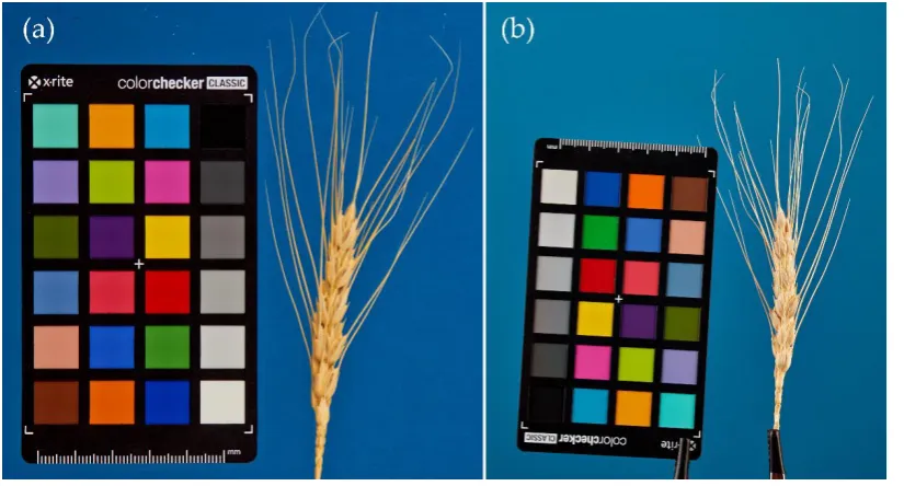
The imaging protocols for further analysis of spikes were proposed earlier [22]. The spike is captured on a blue background (‘table’ protocol) or is vertically fixed with a clip holder (‘clip’ protocol). The holder allows spikes to be fixed at different angles relative to the spike axis. Each image contains a ColorChecker Mini Classic target (https://xritephoto.com/camera) for color correction. This correction allows for avoiding color shifts in the images, which result from differences in the lighting conditions [23]. Another advantage in using the color scale is its standard size (68 × 108 mm), allowing for assessment of image scale.
Figure 1. Images of spikes captured by two different protocols: (a) on a table and (b) fixed with a clip holder.
2.2. Identifying Spike and Awns in Images 2.2.1. Image Preprocessing
Images were processed using the OpenCV (Open Source Computer Vision Library; https://opencv.org) software package [24]. At the first stage, we identified the color scale for the image (Figure 1, left). The color scale may be tilted relative to the image vertical axis and its plane is not always perpendicular to the optical axis of the lens in the case of ‘clip’ protocol. The scale was identified using its reference image to identify several descriptors by searching for key points. The descriptor in the spike image closest in the Hamming distance was determined for each descriptor of the reference image. The regions corresponding to different colors of the palette were identified by aligning a calibrated image of the scale with the reference one using a RANSAC algorithm [24].
Having identified the color scale, we correction the image color with the help of a method used in epiluminescence microscopy [25]. The shift in colors in spike image relative to the reference was assessed using Dcol parameter: the higher its value, the more significant is the color distortion. If Dcol is close to zero, the image contains almost no color distortion. For details of the algorithm of color scale identification and correction, see Supplementary file (Section 1.2).
The image scale (pixel size, mm) was calculated from the ratio of the known color scale area to its area in the image (taking into account the correction for its orientation). Further, the ColorChecker area was excluded from analysis.
At the next stage of image preprocessing, we blurred the image using a Gaussian filter to reduce noise and removed the fragments of clip holder (for ‘clip’ protocol).
2.2.2. Image Binarization
2.2.3. Awn Identification
The awns are colored similar to the spike. In some images, awns intensively intersect and even stick together forming a bundle, which significantly hinders identification of individual awns and even makes it impossible in some cases. Correspondingly, a two-stage algorithm was used.
At the first stage, the pixels of the awn skeleton are identified. Since the awns are much thinner as compared with the spike region (body), a partial skeletonization algorithm was used for identifying the awn skeleton [26]. The pixels at the spike–background boundary were iteratively erased with retention of the connectivity of spike and awn regions so that the erasure of each next pixel at the spike contour did not increase the number of isolated spike regions in the image. To stop the algorithm, the threshold of iterations was used; this threshold was selected using a training sample of images (see below). In the course of erasure, the sequence of erased pixels of the contour was saved. This further allowed for determination of the pixels the erasure of which led to formation of the skeleton. These pixels were denoted as the pixels of awns.
2.2.4. Selecting Parameters for Identification of Spike and Awn Regions in Image
Operation of the algorithm for identification of spike and awn regions depends on the following parameters:
(1) The target values of HSV channels and the ranges of their acceptable deviation for image binarization into the background and spike/awn regions and
(2) The number of iterations (n) to the stoppage of skeletonization algorithm.
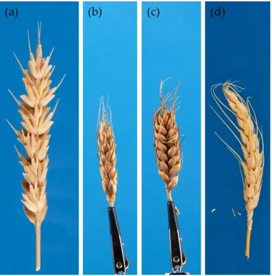
Figure 2. Awnedness types of spikes: (a) awnless, (b) awnletted, (c) half-awned, (d) and short-awned. Table 1. Distribution of the spikes in sample according to awnedness types.
Awnedness type Number of images
‘Clip’ protocol
‘Table’ protocol
Awnless 16 10 6
Awnletted 4 4 0
Half-awned 14 14 0
Short-awned 59 36 23
The Jaccard index, J [27], was used for assessing performance of the algorithm for image segmentation into the background and spike:
𝐽(𝐴, 𝐵) =|𝐴 ∩ 𝐵|
|𝐴 ∪ 𝐵|=
|𝐴 ∩ 𝐵| |𝐴| + |𝐵| − |𝐴 ∩ 𝐵|
(crossing over) target colors with linked ranges. The population size varied from 20 to 100 individuals.
2.2.5. Awn Quantitative Characteristics
Once the awn and spike regions are selected, the characteristics of spike awnedness are calculated, including the total awn area, Sa (mm2), determined as the number of the corresponding pixels multiplied by the area of 1 pixel; the number of awns, Na, as the number of contacts between spike and awn regions (number of awn bases); total awn length, La (mm), as the total length of the pixels that from the skeleton of awn region; and the mean awn length, la = La/Na (mm). Since part of the images contained considerably intersected and/or overlapped awns, it was impossible to distinguish individual awns; correspondingly, we did not assess the lengths of individual awns (Fig. 2B–D).
2.3. Spike Morphometry
2.3.1. Identifying and Straightening Spike Contour
Broken lines were sometimes formed after awn erasing at the sites where they contacted the spike body. In this case, we smoothed the contour using an algorithm for computing elliptic Fourier descriptors [29]. After the awn regions were removed, descriptors for 70 harmonics were computed to recognize the spike contour and further use them for determining the points of smoothed contour. The spike axis was approximated with a broken line iteratively constructed of the segments of spike body. At the first stage, the center of mass and the main axes of the ellipsoid approximating the contour were determined for the pixels of the contour. The major axis corresponded to the direction of the rachis in the center of mass. The perpendicular to the major axis divides the spike region into two parts. At the second stage, an analogous procedure was applied to each part. As a result, each part was also divided by the corresponding axis into two parts; the next iteration stage was again applied to each part. The procedure was successively performed until the number of segments exceeded 20. The centers of mass of each constructed segment determined the broken line that approximated the spike axial line. At the last stages of iteration, the segment size across the axis in some cases could be larger than along the axis. In this case, an axis codirectional to the major axis of the segment constructed at the previous stage but passing the center of mass of the current segment was used as the axis of this segment.
After the spike axial line is determined, the spike contour is straightened so that this axis is vertical with its upper end at the spike tip and its lower end, at its base and the distance of the pixels of the transformed contour from the axial line are equal to the distances of the corresponding pixels of the initial contour. This transformation makes it possible to remove the deformation of spike contour caused by its bending. The size and quantitative characteristics of spike shape are determined in the straightened spike contours.
2.3.2. Integral Characteristics of Spike Shape
The characteristics of spike shape fall into several categories. The first group comprises integral shape characteristics, such as spike length Le (mm), which is approximated by the length of spike axial line; Pe (mm), the perimeter of spike without awns; Se (mm2), the area of spike region; and square index, SQI = Se/(L2), the ratio of the spike area to its squared length.
The other integral parameters are described below.
Circularity index 𝐼 reflects the degree to which the shape of the contour is close to a circle; its value varies from 0 to 1, with the unity value for an ideal circle:
𝐶 =4𝜋 × 𝑎𝑟𝑒𝑎
𝑝𝑒𝑟𝑖𝑚𝑒𝑡𝑒𝑟2
𝑅 = 4 × 𝑎𝑟𝑒𝑎
𝜋 [𝑀𝑎𝑗𝑜𝑟 𝑎𝑥𝑖𝑠]2
Rugosity index, Rg, is determined as the ratio of the perimeter of the contour to the convex perimeter:
𝑅𝑔 =𝑃𝑠
𝑃𝑐
where Ps is the perimeter of the contour and Pc, its convex perimeter, also known as the least convex hull, i.e., the least convex figure that contains all points of an image.
Solidity index, S, is the ratio of the contour’s area to the area of its convex hull:
𝑆 = 𝐶𝑜𝑛𝑡𝑜𝑢𝑟 𝐴𝑟𝑒𝑎
𝐶𝑜𝑛𝑣𝑒𝑥 𝐻𝑢𝑙𝑙 𝐴𝑟𝑒𝑎
2.3.3. Model of Sections
The very first model for describing the spike shape was a set of sections determined by the perpendiculars to spike’s axial line with a step of 1/21 of the spike length. Two distances for the pixels of the contour were determined for each perpendicular (from each side of the axial line). Thus, this model was defined by 40 parameters.
2.3.4. Model of Quadrilaterals
The contour of a spike placed horizontally is representable as two quadrilaterals (Figure 3)— upper and lower ones with a common base. The left and right sets of edges are approximated by two quadrilaterals with one adjacent side, their base, being equal to the sum of the spike axis intervals (spike length Le). The geometry of the upper quadrilateral is determined by the four following independent parameters (Figure 3):
xu1 is the distance from the spike tip to projection B’ of top B onto base AD; xu2 is the distance of B’ to projection C’ of top C onto base AD;
yu1 is the distance of top B to its projection B’ onto base AD; and yu2 is the distance of top C to its projection C’ onto base AD;
Distance xu3 from projection C’ to spike base D is computable from the spike length as xu3 = Le – xu2. Analogous parameters xb1, xb2, xb3,yb1, and yb2 are determined for the lower (bottom) quadrilateral (Figure 3).
The parameters of the upper and lower quadrilaterals were selected so that to minimize the squared deviation of the height between the pixels of the contour and edges of the quadrilateral. The Levenberg–Marquardt algorithm [30] implemented in the Apache library (class org.apache.commons.math3.fitting.leastsquares.LevenbergMarquardtOptimizer) was used for minimization.
Figure 3. Representation of the spike shape as two quadrilaterals. Black horizontal line shows the spike axial line; brown line, spike contour; and green lines, quadrilaterals approximating spike contour. The main parameters characterizing its geometry are shown for the upper quadrilateral.
αu1 is the inclination of edge AB relative to the base of the upper quadrilateral (degrees);
αu2 is the inclination of edge BC relative to the base of the upper quadrilateral (degrees);
αu3 is the inclination of edge CD relative to the base of the upper quadrilateral (degrees); t1u is the tangent of angle αu1;
t2u is the tangent of angle αu2; t3u is the tangent of angle αu3;
Su1 is the area of triangle ABB’ (mm2); Su2 is the area of trapezium BB’C’C (mm2); Su3 is the area of triangle DCC’ (mm2);
Su is the area of the upper quadrilateral (mm2); and yum is the mean height of the upper quadrilateral (mm).
The parameters for the lower quadrilateral were calculated in an analogous manner. The following variables were also calculated for both quadrilaterals:
AIx2 = (xu1 – xb1)2/xu1 + (xu2 – xb2)2/xu2 + (xu3 – xb2)2/xu3 is the asymmetry index for the lengths of segments (mm);
AIy2 = (yu1 – yb1)2/yu1 + (yu2 – yb2)2/yu2 is the asymmetry index for the heights of the segments (mm); and AIxy2 = AIx2 + AIy2 is the total asymmetry index (mm).
2.3.5. Radial Model
Parameters of the radial model are calculated as follows: 360 rays are drawn from the center of mass of the spike contour starting from the direction of its major axis with a step of 1 degree to the point of the contour closest to a given ray. The lengths of the 360 intervals thus constructed represent the radial model.
The total list of all spike morphometric characteristics is shown in Supplementary file (Table S1). 2.4. Predicting Spike Density Index and Type of Its Shape
2.4.1. Sample of Spike Images
We assessed the efficiency of our approach by prediction the spike shape type. For this purpose, the spike images of 249 plants, annotated manually, were extracted from the SpikeDroid database [22]. We used digitalized data of 1245 spike images of eight hexaploid wheat species, one artificial amphyploid and one intraspecific F2 hybrid population (Table 2). These wheat species have the spikes of contrasting shapes, which are controlled by well-studied genes [31]. The main spike of each plant was chosen; five images of each spike were acquired in one projection using a ‘table’ protocol and four, using a ‘clip’ protocol).
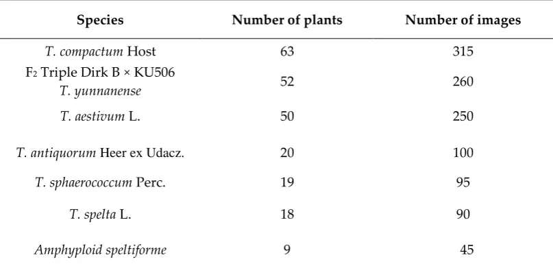
Table 2. Wheat species and hybrids used in prediction of spike density index and shape type.
Species Number of plants Number of images
T. compactum Host 63 315
F2 Triple Dirk B × KU506
T. yunnanense 52 260
T. aestivum L. 50 250
T. antiquorum Heer ex Udacz. 20 100
T. sphaerococcum Perc. 19 95
T. spelta L. 18 90
T. yunnanense 9 45
T. macha Dekapr. et Menabde 9 45
For each plant, the spike shape type was determined by an expert, its length was measured, and the number of spikelets per spike was counted. According to spike shape type, 110 plants were ascribed to the group with compact spikes; 72 plants, to normal; and 67 to spelt. Examples of the images of each spike shape type are shown in Supplementary file (Figure S2). Density index D [32], where (A – 1) is the number of spikelets per spike without the apical spikelet and B, the length of spike rachis (cm), displays a high correlation with spike shape.
𝐷 =10(𝐴 − 1)
𝐵
2.4.2. Methods for Predicting Spike Characteristics
To predict the density index, we used the random forest method (RandomForestRegressor, sklearn.ensemble software package, scikit-learn library [33]). The spike shape type was determined with the help of LogisticRegression and RandomForestClassifier of the same library.
For prediction, we used 44 parameters of the quadrilateral model and seven indices that describe the spike geometric characteristics (perimeter, spike area, total awn area, circularity index, roundness, solidity, and rugosity). The number of parameters for the model of sections and radial model was reduced to 10 using principal component analysis (the largest components were selected from the sample in Table 2 so that they finally accounted for over 90% of variations). Thus, we analyzed 71 parameters for each image.
In the case of ‘clip’ protocol, each spike is represented in four projections. We pooled the parameters of all four images by ranking projections according to a decrease in spike width (parameter yum). As a result, we got 284 parameters (parameters 1 to 142 describe the frontal side of the spike and 143 to 284, its lateral side).
To estimate the characteristics of spike shape, we selected the most significant parameters according to their predictive capacity for spike density estimation. The parameters were ranked according to their significance based on the averaged results of eight different approaches: (1) linear regression coefficients (Linear Regression); (2) regression coefficients with lasso regularization (Lasso); (3) regression coefficients with ridge regularization (Ridge); (4) selection of parameters according to stability criterion [34] using RandomizedLasso, sklearn library (Stability); (5) ranking according to recursive feature elimination (RFE) [35]; (6) ranking based on average entropy reduction computed when constructing the trees of solutions by random forest method (RF) using RandomForestRegressor class, sklearn.ensemble software package; (7) ranking based on the correlation between regressor and target parameters (Corr) using f_regression class in sklearn.feature_selection package; and (8) ranking based on the maximal information coefficient (MIC), which takes into account nonlinear dependences between parameters [36] using the MINE (maximal information-based nonparametric exploration) statistics of minepy package. The estimate for a parameter in all these strategies varies in the range of 0 to 1.
2.4.3. Assessing Prediction Performance
To estimate prediction performance for density index, we used the mean absolute error (MAE) and mean absolute percent error (MAPE), calculated as
MAE = 𝑀1∑ |𝑛𝑗− 𝑛′𝑗| 𝑗 = 𝑀
𝑗 = 1
MAPE = 100%
𝑀 ∑ (|𝑛𝑗− 𝑛
′ 𝑗|/𝑛𝑗) 𝑗 = 𝑀
where M is the number of spikes; nj is the density index calculated manually; and n’j is the predicted density index value. In addition, we assessed the Pearson correlation coefficient for predicted and expert-assessed values.
The prediction performance for spike classification according to their shape was assessed using measure F1, calculated as the mean harmonic for precision and recall [37]:
𝐹1 = 2Precision × Recall
Precision + Recall
Precision = 𝑇𝑃
𝑇𝑃 + 𝐹𝑃
Recall = 𝑇𝑃
𝑇𝑃 + 𝐹𝑁
where TP, TN, FP, and FN correspond to the number of true positive, true negative, false positive, and false negative solutions.
The data were divided into training and test samples at a ratio of 70 to 30%. The prediction accuracy was assessed using cross-validation. The MAE, MAPE, and F1 values were averaged over five iterations of the cross-validation for both the training and test samples.
2.5. Analysis of F2 hybrid plants
We analyzed F2 hybrids between the near-isogenic line of Australian common wheat cultivar Triple Dirk (Triple Dirk B) and the Chinese wheat Triticum yunnanense, King ex S.L. Chen (syn. T. spelta ssp. yunnanense (King ex S.L. Chen) N.P. Gontsch.), accession KU 506. The sample includes 120 plants grown in the hydroponic greenhouse with standard air humidity, temperature and light conditions. Triple Dirk B plants have normal ear shape, while KU 506 was characterized by dense spelt ones. Main spike images of these plants were obtained using ‘table’ protocol.
3. Results
3.1. Assessing the Recognition Accuracy for Awn and Spike Regions
After selecting the optimal parameters for the algorithm, the achieved recognition accuracy of spike body and awns for the test sample were Jb = 0.925 and Ja = 0.660, respectively, and for the training sample, Jb = 0.932 and Ja = 0.634.
Color correction had no significant effect on the recognition accuracy of spike and awns: the mean Jaccard index, Jb, for the spike body segmentation with color correction was 0.925 and for awns with color correction, mean Ja was 0.679.
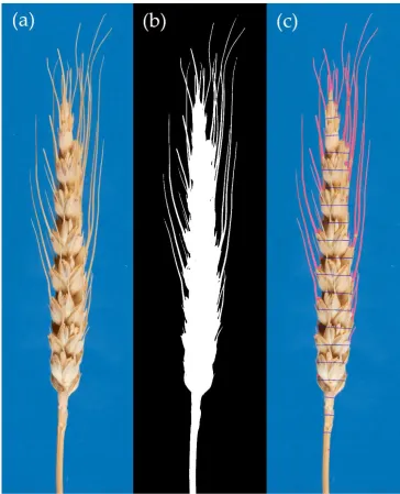
Figure 4. Stages of the algorithm for identifying awns by the example of spike ID no. 6450: (a) spike image on blue background; (b) binarized spike pattern; and (c) initial spike image with recognized awn regions (marked red) and spike sections (marked blue).
We estimated the effects of various factors associated with the protocols of image acquisition and processing on the accuracy of awn identification, including the scale of imaging (number of pixels per unit captured area), type of the protocol (‘table’ or ‘clip’), and spike projection (front or side) for the latter protocol.
First and foremost, we studied the effect of image scale on the accuracy of awn identification. As has emerged, the sample of images that we used for assessing the accuracy of detecting the contours contains four scales (Supplementary file, Figure S1). All images acquired using the ‘table’ protocol reside along one line (scale 4, orange circles). The remaining scale variants correspond to the images of the ‘clip’ protocol. Thus, the differences in the image scales are inevitable for these protocols and the use of the color scale for determining the image scale is justified.
Figure 5. Distribution of Jaccard index J for (a) the awns and (b) spike bodies grouped according to imaging scale.
The estimate for the recognition accuracy of awn regions, Ja, falls into the range of 0.27–0.9. For scale 1, the distribution of accuracy is shifted towards the smaller side (Figure 5) and amounts on the average to approximately 0.549; this is logical since it is the largest imaging scale. As for the remaining scales (scales 2, 3 and 4), the Ja distributions differ to a lesser degree: their mean values are 0.695, 0.607, and 0.676, respectively. The recognition accuracy for the spike body, Jb, falls into the range of 0.8–0.98 with means of 0.901, 0.928, 0.938, and 0.945 for scales 1–4, respectively. Note that Jb displays the evident trend of an increase in the recognition accuracy of spike body with a decrease in the scale, unlike Ja.
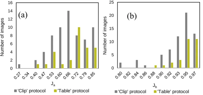
The second factor putatively influencing the algorithm performance is the types of the used protocol. In the ‘table’ variant, the distance between the camera and object in a set of shots is fixed, while the spike is placed horizontally on the surface of a table in the plane perpendicular to the lens axis. In the case of ‘clip’ protocol, the spike may deviate from the plane perpendicular to the lens axis because it is bent or fixed along the axis differing from the vertical. We analyzed the distribution of J for the images grouped according to the used protocols (Figure 6).
Figure 6. Distribution of the Jaccard indices, J, for (a) awns and (b) spike body grouped according to the used protocols (‘clip’ or ‘table’).
0 0.05 0.1 0.15 0.2 0.25 0.3 0.35 0.4 0.45 0.5 P erc en tag e of i m ag es Ja
Scale 1 Scale 2 Scale 3 Scale 4
0 0.1 0.2 0.3 0.4 0.5 0.6 0.7 P erc en tag e of i m ag es Jb
Scale 1 Scale 2 Scale 3 Scale 4
0 2 4 6 8 10 12 14 16 Num be r of i m ag es Ja
'Clip' protocol 'Table' protocol
0 5 10 15 20 25 Num be r of i m ag es Jb
'Clip' protocol 'Table' protocol
(a)
(b)
The results shown in Figures 5 and 6 demonstrate that the image scale significantly influences the recognition accuracy of both the spike body and awns and the type of used protocol has a significant effect on the identification accuracy for spike body but not for awns.
3.2. Analyzing Awnedness Parameters for Spike Sample
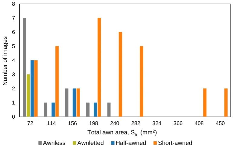
We have analyzed the total awn area (mm2), Sa. The significant differences between Sa distributions for a sample of 46 images (without repeating different projections) were observed for the images of awnletted and short-awned spikes (χ2 = 22.64, p < 0.05); awnless and short-awned (χ2 = 24.75, p < 0.05); and short-awned and half-awned (χ2 = 18.09, p < 0.05).
Figure 7 shows the distribution of the awnedness types relative to Sa: the short-awned spikes have the largest range; note that they have both large and small values of the total awn area. The largest number of spike images with this awnedness type has a medium area value (180 < Sa < 222 mm2). The awnletted spikes have the minimum total awn area followed by the awnless and half-awned spikes. However, the obtained Sa distributions for different spike shape types considerably overlap, with only one Sa interval housing a single awnedness type, short-awned spikes (264 mm2 < Sa).
Figure 7. Histogram of the spike distribution according to awnedness type for the sample used to compute total awn area.
3.3. Predicting Density Index and Type of Spike Shape 0
1 2 3 4 5 6 7 8
72 114 156 198 240 282 324 366 408 450
Num
be
r
of
i
m
ag
es
Total awn area, Sa (mm2)
Awnless Awnletted Half-awned Short-awned
Figure 8. (a) Histogram of spike distribution according to density index and (b) diagram of spike distribution according to the number of spikelets per spike and spike length.
The distribution of spikes from the samples shown in Table 2 according to the manually assessed density index is shown in Figure 8. As is evident, the compact spikes display high density for spelt spikes, of 10–30. The distributions of the last two types considerably overlap. An analogous significant overlapping of the distributions of the number of spikelets and spike length is observable for these spike shape types (Figure 8B). It is also evident that these distributions for the compact spikes are considerably different.
To predict the spike density, we selected variables characterizing spike morphology using several criteria (as is described in 2.4.2). The variables were ranked based on the averaging of eight significance characteristics. Then, the variables were added one by one in the descending order of mean significance value using both training and test samples. Regression was performed using the random forest method. While adding variables, the MAE values were assessed for the test and training data.
The training involved 12 most significant parameters The number of parameters for training was selected based on the training curves (Supplementary file, Figure S3), showing the dependence of MAE in predicting spike density index on the number of best parameters used for training by random forest method.
We ranked the parameters according to their significance when predicting the spike density index. The results of selection of the 12 best parameters for ‘table’ (one projection) and ‘clip’ (four projections) protocols are listed in Tables 3 and 4, respectively.
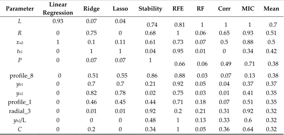
Table 3. Estimation of the measures of significance of spike quantitative characteristics for predicting spike density based on analysis of the images acquired by ‘table’ protocol: characteristics are listed in column 1; significance values, in columns 2–9; and their means, in column 10. The significance measures are described in Methods, section 2.4.2.
Parameter Linear
Regression Ridge Lasso Stability RFE RF Corr MIC Mean
L 0.93 0.07 0.04
0.74 0.81 1 1 1 0.7
R 0 0.75 0 0.68 1 0.06 0.65 0.93 0.51
xu2 1 0.1 0.11 0.61 0.73 0.07 0.5 0.88 0.5
tb1 0 1 1 0.04 0.95 0.01 0 0.34 0.42
P 0 0.07 0.07 1
0.66 0.06 0.49 0.71 0.38 profile_8 0 0.51 0.55 0.86 0.88 0.03 0.07 0.13 0.38
yb1 0 0.7 0.7 0.21 0.92 0.05 0.04 0.37 0.37
yu1 0 0.82 0.78 0.02 0.75 0.03 0.01 0.41 0.35
profile_1 0 0.46 0.45 0.44 0.71 0.18 0.07 0.51 0.35
radial_3 0 0.01 0.01 0.92 0.2 0.21 0.31 0.92 0.32
yb2/L 0 0 0 0.48 1 0.13 0.33 0.6 0.32
C 0 0.2 0 0.34 1 0.05 0.36 0.64 0.32
values, in columns 2–9; and their means, in column 10. The significance measures are described in Methods, section 2.4.2.
Parameter Linear
Regression Ridge Lasso Stability RFE RF Corr MIC Mean
xb2 (projection 2)
1 0.15 0.13 0.75 1 0 0.46 0.68 0.52
xu2 (projection 2) 0.98 0.06 0.04 0.87 0.9 0.04 0.63 0.63 0.52
C (projection 3) 0 0.24 0 0.81 0.53 1 0.62 0.94 0.52
yb1/L (projection 3) 0 0.01 0 0.9 0.59 0.86 0.86 0.8 0.5
R (projection 3) 0 0.38 0 0.94 0.64 0.01 0.84 0.96 0.47
L (projection 4) 0.42 0.06 0.01 0.5 1 0.01 0.79 0.79 0.45
R (projection 4) 0 0.32 0 0.88 0.52 0.01 0.81 1 0.44
yu1/L (projection 3) 0 0.01 0 0.94 0.71 0.02 1 0.71 0.42
L (projection 3) 0.11 0.08 0.02 0.26 1 0.2 0.73 0.76 0.4
yu1/L (projection 4) 0 0.01 0 1 0.48 0.01 0.84 0.8 0.39
R (projection 2) 0 0.19 0 0.8 0.49 0.03 0.63 1 0.39
xu2 (projection 1) 0.58 0.05 0 0.52 0.73 0.03 0.43 0.65 0.37
The parameters with a high significance for both protocols are spike length and circularity index. Interestingly, these traits appear significant for almost all projections in the case of ‘clip’ protocol.
The accuracy estimates for the prediction of density index and spike shape type (spelt, normal, or compact) are listed in Table 5. The training involved the parameters listed in Table 3 for the images acquired according to ‘table’ protocol and in Table 4 for the ‘clip’ images. The mean absolute error in predicting density index in the test sample (MAE test) is 4.61 for one projection and 3.33 for four projections. The Pearson correlation coefficient for the predicted values and expert estimates in the test sample (R) is 0.51 for one projection and 0.74 for four projections. The classification models were trained by logistic regression (lr) and random forest (rf) methods.
Table 6 lists the accuracy estimates for the prediction of spike shape type. We attempted to use the predicted density index (lr_density_pred and rf_density_pred) as an additional trait but got no gain in accuracy. The values of F1 measure for performance of spike shape classification in test sample is 0.85 (F1_rf) for four projections and 0.78 (F1_lr) for one projection. These accuracy estimates demonstrate that utilization of the information about four projections increases the prediction performance by 7% and decreases MAE for spike density prediction by 1.28, which corresponds to 4.25%.
Table 5. Estimates of prediction performance for of spike density index for one (‘table’) and four (‘clip’) projections (MAEtraining and MAEtest, mean absolute errors for training and test samples; MAPEtraining and MAPEtest, mean absolute percent errors for training and test samples; R2training and R2test, Pearson correlation coefficient between the predicted and expert estimates for training and test samples).
Performance measure ‘Clip’ ‘Table’
MAEtraining 1.48 1.88
MAEtest 3.33 4.61
MAPEtraining 6.19 7.77
MAPEtest 13.28 17.80
R2training 0.95 0.94
R2test 0.75 0.52
according to density by logistic regression and random forest methods; F1 lr_density_pred and F1 rf_density_pred, the F1 measure for the classification accuracy using an additional parameter, predicted density index, by logistic regression and random forest methods).
Performance measure ‘Clip’ ‘Table’
F1_lr 0.82 0.78
F1 lr_density_pred 0.83 0.77
F1_rf 0.85 0.72
F1 rf_density_pred 0.84 0.76
Table 7 lists the estimates of confusion matrix values for the classification of spike shape in the test sample for four projections obtained by random forest method. It is evident that compact and spelt spikes are distinguished with the least number of errors. As for the normal spikes, they are most frequently predicted as belonging to two other types (lowest prediction quality). Interestingly, the spikes belonging to normal and spelt ones give the highest number of mutual false predictions. These results agree with the histograms in Figure 8A, which are based on expert estimates.
Table 7. Confusion matrix for classification of spike shape in the test sample of images in four projections (‘clip’ protocol).
Compact observed Normal observed Spelt observed
Compact predicted 158 13 0
Normal predicted 8 79 20
Spelt predicted 0 20 77
3.4. Analysis of F2 hybrid plants
Figure 9. The distribution of the spike density values predicted using 2D images for F2 hybrids between the near-isogenic line of Australian common wheat cultivar Triple Dirk (Triple Dirk B) and the Chinese wheat Triticum yunnanense, King ex S.L. Chen (syn.. T. spelta ssp. yunnanense (King ex S.L. Chen) N.P. Gontsch.), accession KU 506.X axis is the density index, Y axis is the percentage of spikes. Arrows points to the parent D values, 20.40 for Triple Dirk B and 29.66 for KU 506.
4. Discussion
In this paper, we proposed a method that makes it possible to
– Recognize a spike pattern in the images acquired using two standard protocols [22]; – Separate the awns from spike body in images;
– Estimate quantitative characteristics of spike awnedness (total awn area in image, awn number, and mean length); and
– Estimate quantitative characteristics of spike shape, both integral and describing the shape as ad-hoc models.
Analysis of the identification performance for spike region has shown that the image scale has the most significant effect on the background/spike and spike body/awns segmentation accuracy: the farther the spike from the camera lens, the higher is the segmentation error. The imaging scale considerably differs depending on the protocol for image acquisition; in ‘table’ protocol, camera is considerably closer to the object, while in ‘clip’ variant, the distance to the object may vary. Since the focal length was fixed, the scale depended only on the distance to the imaged object.
Color correction of images has no significant effect on the segmentation accuracy. Most likely, this is the result of standard illumination during spike capturing [22]. Nonetheless, the option of color correction, available in our method, allows the colors in images to be more objectively estimated and assists in considerable improvement of data processing under conditions of poorly controllable illumination.
spike body region. In addition, the very manual marking of high resolution images is laborious and does not allow the fluctuations in identification of spike boundaries to be avoided.
Here, we propose a method for assessing the parameters of spike shape. These parameters are arbitrary dividable into “general” characteristics reflecting the overall shape (for example, spike circularity, area, and length). We also additionally introduced the ad-hoc models for description of spike shape. Two of them (model of sections and radial model) were formulated based on most general considerations and their parameters have no specificity associated with the typical wheat spike shape. The third model, which describes the spike as two quadrilaterals with a common side, may be a more illustrative generalization of spike shape. The fact that a considerable number of parameters used in this model are among those significant for predicting the spike density (Tables 3a and 3b) suggests that this model is the most adequate. The general spike characteristics and the parameters of the model of quadrilaterals are prevalent among the significant parameters. Figure S2 (Supplementary file) shows how the model approximates two quadrilaterals for the spikes of different shapes as well as the indices with the largest contributions to density index predictions,
In our work, we have assessed the prediction accuracy for spike density and shape type based on the quantitative characteristics obtained by analyzing spike images. Two regression methods— logistic regression and random forest—were selected since the volume of training sample (in our case, ~200 spikes) is not critical for them as compared with neural networks or deep learning neural networks, which require thousands and tens of thousands of images to gain a good result [19].
The logistic regression–based prediction of spike density gives a MAE value of 4.61 (using one spike image projection). The prediction accuracy increases (MAE = 3.33) when the data for four projections are used although the number of parameters for prediction remains the same (however, these 12 parameters include the characteristics obtained by analyzing different spike projections).
The accuracy of spike shape classification into three types (spelt, normal, and compact) using the random forest algorithm (F1 measure) is 0.78 for one spike projection and 0.85 for four projections. Interestingly, the latter value is close to the estimate for classifying spikes of four wheat varieties by Kun et al. [21], which amounts to 0.88 (neural networks using 12 input parameters). A difficulty in solving this problem is that the spelt and normal spikes may be rather similar, as is shown, in particular, by a considerable overlapping of the corresponding spike density distributions (Figure 8). Further accumulation of annotated images and use of deep learning neural network methods will be helpful in solving this problem.
Results of F2 hybrid plants demonstrated high correlation between spike length values estimated manually and from 2D image analysis. This allows us to hope for the effective use of the proposed method to assess the character of the hybrid segregations in interspecific wheat hybridization. 5. Conclusions
An algorithm for identification of spike in a 2D image acquired by a standard protocol is proposed as well as for quantitative description of spike shape using both its integral characteristics (spike length, width, and circularity) and the parameters of three ad-hoc models. The information on spike morphometric characteristics gained as a result of analysis may be useful for high-throughput automated phenotyping, breeding and genetics experiments.
The performed assessment of prediction performance is sufficient for spike pattern recognition in automated harvesting of spike morphometry data.
Although the accuracy in recognizing the awn regions is not too high as compared with the manual patterns, this approach may be helpful for verification of the annotation of available spike images.
The segmentation of the overall spike into total awn and spike body regions may significantly improve the estimate of spike shape by eliminating the distortions of the spike pattern caused by awns.
pixels of awns to the total awn area (mm2) grouped according to imaging scale. Figure S2-4. Stages of algorithm operation for compact, normal and spelt spikes. Figure S5. Dependence of the mean absolute error (MAE) in predicting spike density index on the number of best parameters used for training with random forest method. Figure S6. Scatterplot diagram for the main spike length for Triple Dirk B × KU506 F2 hybrid plants estimated manually (X axis) and from the 2D image analysis (Y axis).
Acknowledgments: The work was supported by the Russian Science Foundation (project no. 17-74-10148). Bioinformatics data analysis was performed with the help of computational resources of the Bioinformatics Joint Access Center, supported by budget project no. 0324-2019-0040.
Author Contributions: Conceptualization, M.A.G., D.A.A. and N.P.G.; methodology, M.A.G., E.G.K. and D.A.A.; software, E.G.K., N.V.S. and M.A.G.; validation, E.G.K. and M.A.G.; formal analysis, M.A.G.; investigation, M.A.G., E.G.K. and N.V.S.; resources, Y.V.K., and N.P.G.; data curation, Y.V.K. and N.P.G.; writing—original draft preparation, M.A.G, E.G.K. and D.A.A.; writing—review and editing, M.A.G., N.P.G. and D.A.A.; visualization, M.A.G. and E.G.K.; supervision, D.A.A. and N.P.G.; project administration, M.A.G.; funding acquisition, M.A.G.
Conflicts of Interest: The authors declare no conflict of interest. References
1. Dorofeev, V.F.; et al. Тhе intеrnаtiоnаl соmесоn list оf dеsсriрtоrs fоr thе gеnus Тritiсum L.; VIR: Russia, Leningrad, 1984. (in Russian)
2. Konopatskaia, I.; Vavilova, V.; Blinov, A.; Goncharov, N.P. In Spike morphology genes in wheat species (Triticum L.). Proceedings of the Latvian Academy of Sciences. Section B. Natural, Exact, and Applied Sciences2016, 70(6), 345-355 [CrossRef].
3. Goncharov, N.P. Genus Triticum L. taxonomy: the present and the future. Plant Systematics and Evolution
2011, 295 (1-4), 1-11 [CrossRef].
4. Börner, A.; Schäfer, M.; Schmidt, A.; Grau, M.; Vorwald, J. Associations between geographical origin and morphological characters in bread wheat (Triticum aestivum L.). Plant Genetic Resources2005, 3 (3), 360-372
[CrossRef].
5. Guo, Z.; Zhao, Y.; Röder, M.S.; Reif J.C.; Ganal M.W.; Chen D.; Schnurbusch T. Manipulation and prediction of spike morphology traits for the improvement of grain yield in wheat. Scientific reports 2018, 8(1)
[CrossRef] [PubMed].
6. Goriewa-Duba, K.; Duba, A.; Wachowska, U.; Wiwart, M. An Evaluation of the Variation in the Morphometric Parameters of Grain of Six Triticum Species with the Use of Digital Image Analysis.
Agronomy2018, 8 (12), 296 [CrossRef].
7. Hammer, K.; Filatenko, A.A.; Pistrick, K. Taxonomic remarks on Triticum L. and × Triticosecale Wittm. Genet. Resour. Crop. Ev.2011, 58 (1), 3-10 [CrossRef].
8. Matsuoka Y.; Nishioka E.; Kawahara T.; Takumi S. Genealogical analysis of subspecies divergence and spikelet-shape diversification in central Eurasian wild wheat Aegilops tauschii Coss. Plant Syst. Evol.2009, 279, 233–244 [CrossRef].
9. Li, Y.; Cui, Z.; Ni, Y.; Zheng, M.; Yang, D.; Jin, M.; Chen, J.; Wang, Z.; Yin, Y. Plant density effect on grain number and weight of two winter wheat cultivars at different spikelet and grain positions. PloS one2016, 11 (5), [CrossRef] [PubMed].
10. Afonnikov, D.; Genaev, M.; Doroshkov, A.; Komyshev, E.; Pshenichnikova, T. Methods of high-throughput plant phenotyping for large-scale breeding and genetic experiments. Russian journal of genetics2016, 52 (7), 688-701 [CrossRef][PubMed].
11. Giuffrida, M. V.; Chen, F.; Scharr, H.; & Tsaftaris, S.A. Citizen crowds and experts: observer variability in image-based plant phenotyping. Plant methods2018, 14(1), 12 [CrossRef][PubMed].
13. Tanabata, T.; Shibaya, T.; Hori, K.; Ebana, K.; Yano, M. SmartGrain: high-throughput phenotyping software for measuring seed shape through image analysis. Plant Physiol.2012, 4, 1871–1880 [CrossRef] [PubMed]. 14. Komyshev, E.; Genaev, M.; Afonnikov, D. Evaluation of the SeedCounter, a mobile application for grain
phenotyping. Frontiers in plant science2017, 7, 1990 [CrossRef] [PubMed].
15. Wu, W.; Zhou, L.; Chen, J.; Qiu, Z.; He, Y. GainTKW: A Measurement System of Thousand Kernel Weight Based on the Android Platform. Agronomy2018, 8(9), 178 [CrossRef].
16. Strange, H.; Zwiggelaar, R.; Sturrock, C.; Mooney, S. J.; Doonan, J. H. Automatic estimation of wheat grain morphometry from computed tomography data. Functional Plant Biology2015, 42(5), 452-459 [CrossRef]. 17. Grillo, O.; Blangiforti, S.; & Venora, G. Wheat landraces identification through glumes image analysis.
Computers and Electronics in Agriculture2017, 141, 223-231 [CrossRef].
18. Makanza, R.; Zaman-Allah, M.; Cairns, J.; Eyre, J.; Burgueño, J.; Pacheco, Á.; Diepenbrock, C.; Magorokosho, C.; Tarekegne, A.; Olsen, M. High-throughput method for ear phenotyping and kernel weight estimation in maize using ear digital imaging. Plant methods2018, 14 (1), 49 [CrossRef] [PubMed]. 19. Pound, M.P.; Atkinson, J.A.; Wells, D.M.; Pridmore, T.P.; French, A.P. Deep learning for multi-task plant
phenotyping. In Proceedings of the IEEE International Conference on Computer Vision, ICCVW2017, 2055-2063 [CrossRef].
20. Hughes, N.; Askew, K.; Scotson, C.P.; Williams, K.; Sauze, C.; Corke, F.; Doonan, J.H.; Nibau, C. Non-destructive, high-content analysis of wheat grain traits using X-ray micro computed tomography. Plant methods2017, 13(1), 76 [CrossRef] [PubMed].
21. Bi, K.; Jiang, P.; Li, L.; Shi, B.; Wang, C. Non-destructive measurement of wheat spike characteristics based on morphological image processing. TCSAE2010, 26 (12), 212-216 [CrossRef].
22. Genaev, M.A.; Komyshev, E.G.; Fu, Hao; Koval, V.S.; Goncharov, N.P.; Afonnikov, D.A. SpikeDroidDB - information system for annotation of morphometric characteristics of wheat spike. VOGiS2018, 22 (1), 132-140 (in Russian) [CrossRef].
23. Berry, J. C.; Fahlgren, N.; Pokorny, A. A.; Bart, R. S.; Veley, K. M. An automated, high-throughput method for standardizing image color profiles to improve image-based plant phenotyping. PeerJ2018, 6 [CrossRef]
[PubMed].
24. Kaehler, A.; Bradski, G. Learning OpenCV 3: computer vision in C++ with the OpenCV library. O'Reilly Media, Inc.: 2016.
25. Quintana, J.; Garcia, R.; Neumann, L.A novel method for color correction in epiluminescence microscopy.
Comput. Med. Imag. Grap.2011, 35 (7-8), 646-652 [CrossRef] [PubMed].
26. Abu-Ain, W.; Abdullah, S.N. H.S.; Bataineh, B.; Abu-Ain, T.; Omar, K. Skeletonization algorithm for binary images. Procedia Technology2013, 11, 704-709 [CrossRef].
27. Jaccard, P. The distribution of the flora in the alpine zone. 1. New phytologist1912. 11(2), 37-50 [CrossRef] 28. Whitley D. A genetic algorithm tutorial. Statistics and computing1994, 4, 65-85 [CrossRef].
29. Kuhl, F.P.; Giardina, C.R. Elliptic Fourier features of a closed contour. Computer graphics and image processing
1982, 18 (3), 236-258 [CrossRef].
30. Ranganathan, A. The levenberg-marquardt algorithm. Tutoral on LM algorithm 2004, 11 (1), 101-110, Available online: http://www.ananth.in/Notes_files/lmtut.pdf (accessed on 06 March 2019).
31. Swaminathan, M.; Rao, M. Macro-mutations and sub-specific differentiation in Triticum. Wheat Inf. Serv.
1961, 13, 9-11.
32. Flaksberger, K.A. Pshenitsi-rod Triticum L. (Wheats-genus Triticum L.). Cultivated flora of the USSR. Bread cereals—wheat.; Wulff, E.V., Ed.; Gosselkhozgiz.: Moscow, 1935, pp. 17-434 (in Russian).
33. Pedregosa, F.; Varoquaux, G.; Gramfort, A.; Michel, V.; Thirion, B.; Grisel, O.; Blondel, M.; Prettenhofer, P.; Weiss, R.; Dubourg, V. Scikit-learn: Machine learning in Python. Journal of machine learning research2011, 12, 2825-2830.
34. Meinshausen, N.; Bühlmann, P. Stability selection. Journal of the Royal Statistical Society: Series B (Statistical Methodology)2010, 72 (4), 417-473 [CrossRef].
35. Guyon, I.; Weston, J.; Barnhill, S.; Vapnik, V. Gene selection for cancer classification using support vector machines. Machine learning2002, 46 (1-3), 389-422 [CrossRef].
36. Reshef, D.N.; Reshef, Y.A.; Finucane, H.K.; Grossman, S.R.; McVean, G.; Turnbaugh, P.J.; Lander, E.S.; Mitzenmacher, M.; Sabeti, P.C. Detecting novel associations in large data sets. Science2011, 334 (6062), 1518-1524 [CrossRef] [PubMed].