A Sensor Image Super-Resolution via Advanced Generative Adversarial Network

Article

A Sensor Image Super-Resolution via Advanced

Generative Adversarial Network

Shiping Wang*, Linyuan He, Duyan Bi and Chen Wang

College of Aeronautics Engineering, Air Force Engineering University, Xi’an 710038, China;

[email protected] (L. H); [email protected] (D. B); [email protected] (C. W)

* Correspondence: [email protected]; Tel.: +86-181-0924-6725

Abstract: Complementary Metal-Oxide-Semiconductor (CMOS) is a typical image sensor that has a wide range of applications. However, considering the limitations of the weather condition and hardware cost, it is hard to capture high-resolution images by CMOS sensor. Recently, Super-Resolution (SR) techniques for image restoration has been gaining attentions due to its excellent performance. Under the powerful learning ability, Generative Adversarial Networks (GANs) have been proved to achieve great success. In this paper, we propose the Advanced Generative Adversarial Networks (AGAN) to efficiently correct these issues; 1) we design a Laplacian pyramid framework as pre-trained module, which is beneficial to provide multi-scale features for our input. 2) at each feature block, a convolutional skip-connections network, which may contain some latent information, is significant for generative model to reconstruct a plausible-looking image; 3) considering that edge details usually play an important role in image generation, a novel perceptual loss function is defined to train and seek optimal parameters. It is effective to achieve excellent and compelling quality captured by CMOS sensor. Quantitative and qualitative evaluations have been demonstrated that our algorithm not only fully takes advantage of Convolutional Neural Networks (CNNs) to improve the image quality, but also performs better than previous GAN algorithms for super-resolution task.

Keywords: Super-Resolution; Deep-learning; Generative Adversarial Networks; CMOS sensors

1. Introduction

Complementary Metal-Oxide-Semiconductor (CMOS) [1] has been attracting attentions due to its high sensitivity and low cost. However, CMOS sensor encounters inevitably some problems like illumination and motion blurred when it captures images. These factors may cause reduction in contrast, loss of high-frequency details etc. As Super-Resolution (SR) becomes a hot topic in the computer vision research community, it reconstructs a high-resolution (HR) image from given low-resolution (LR) information. SR has a wide range of applications in medical imaging, security and surveillance where high-frequency details are required on demand. The dilemma of SR is an ill-posed inverse problem since multiple HR patches should be consistent with the given LR patch. To address this issue, additional prior knowledge has to be made regarding the formation of HR images.

Recently, deep-learning methods have exhibited the excellent performance in SR tasks. The data-driven manner has also been used with large improvements in accuracy, which includes convolutional neural networks (CNNs) based methods [2]. For example, the pioneer CNN model for SR has gained considerable attention because of its portable architecture [3]. This method, termed Super-Resolution Convolutional Neural Network (SRCNN), provides compelling quality and outperforms traditional non deep-learning algorithms. After that, lots of follow-up methods have shown their advantages for SR tasks. Kim [4] has deployed gradient clipping and residuals-learning to predict the residuals instead of actual pixels. Lai et al. [5] propose the Deep Laplacian Pyramid Network (LapSRN) by upscaling from small upscaling factor to large upscaling factor. They predict progressively the sub-band residuals ranging from coarse to fine levels. With the further development of CNN, they deploy skip-connections strategy to improve image quality. Deep

Recursive Residual Network (DRRN) jointly utilizes skip-connections to fully exploit the latent information [6].

So far, the convolutional neural networks have become more and more powerful in computer vision applications. However, there are less attention for CNN to discriminate whether the extracted features are robust, on the basis of their potential to train high-dimensional, complex real data [7]. Variational Auto Encoders (VAE) and Generative Adversarial Networks (GANs) have given birth comparing with state-of-the-art algorithms on image processing. VAE [8] is attractive model since they learn complex probability distributions form training data. However, the high-quality images seriously lie on the expressiveness of the inference model. In other words, the VAE are not expressive enough when they train true posterior distribution. The GANs [9] mimic the target distribution by building a generative model. The networks that represent 2 parts of the generator and discriminator to extract features for SR tasks. The algorithm of GAN may be characterized as a two-player minimax game between the generative model, which tries to produce counterfeit without detection, and the discriminative model, which learns to distinguish whether the synthesized images from the generator and the real images from data distribution. On the one hand, a noise variable z can be defined as generative model’s input, then Goodfellow et al. take noise z into model G to generate synthesized images G(z). Furthermore, the parameters of network G can be optimized constantly based on the feedback information given by discriminator. On the other hand, the discriminative model D can be viewed as mappings from data distribution: _{D x( )}dicriminator_{(0,1) . It determines whether the} images from the generator (false, close to 0) or from data distribution (true, close to 1). For discriminative model D, training the parameters of D by fixing generator can classify images. Specifically, they achieve this strategy with the utility of joint 2 adversarial networks. It will achieve a balance when the synthesized images G(z) close to real images from data distribution, and the discriminator D predicts 0.5 between G(z) and real images for most inputs. Both networks of G and D have learned capacity enough, which is called the Nash equilibrium [10]. Unfortunately, some of GAN structures are unstable during training performance, which lead generator to produce some artifacts and nonsensical outputs. Considering that CNN architecture has remarkable performance in terms of feature extraction, we take advantages of CNN to construct our generator, and then utilize a discriminator to test whether the generated images satisfy SR performance.

The main contribution of our network are as follows:

1. Laplacian pyramid. Inspired by Laplacian pyramid framework [11], we utilize multiple sizes instead of single size as our pre-trained module. Trade-off between accuracy and speed, we choose 3 layers to integrate abundant features in our Laplacian pyramid framework. Therefore, we not only add some multi-scale features to our input, but also calculate a fine image from bottom-up layers. It is beneficial to provide richer details for pre-trained module than single input method.

2. Convolutional skip-connections. Some CNN algorithms make significant advantages for SR tasks. Different from cascade network in typical methods, we design a convolutional skip-connections network based on an end-to-end manner. Note that feature maps from intermediate layers may contain some latent information. It is crucial for generative model to generate a plausible-looking image rely on convolutional skip-connections. So, our generator can project some high-frequency details onto synthesized images to fool the discriminator D.

3. Perceptual loss function. Normally, several GAN methods are limited by the instability learning during the training. We propose a perceptual loss function to penalize samples in our adversarial network. Considering that edge details usually play a significant role in image generation, the generator produces synthesized images closer to real images via our loss function. Moreover, our loss function corrects the errors between real images and generated images, which improves the accuracy for discriminator.

algorithm shows excellent performance. Finally, some constructive conclusions have been drawn in section 5.

2. Related work

In this section, we first describe the degradation theory, and then discuss some typical algorithms for SR tasks. This includes non deep-learning methods and deep-learning algorithms. Meanwhile, a brief introduction of SR techniques and some typical GAN algorithms are illustrated. The detailed information of SR will be discussed in following sections.

2.1. Degradation Theory

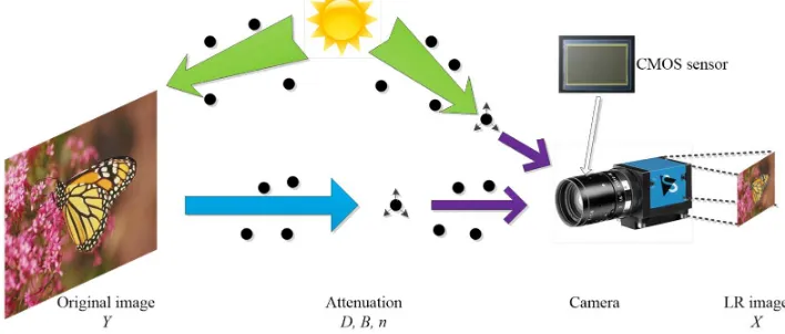
The degradation theory was first presented by McCartney in 1978, which is widely used in computer vision. The theory describes that the images are often subject to degradation factors, such as noise, motion blurred and down-sample operator. In order to reconstruct high quality images, we analyze the degradation model to solve the inverse process of reconstruction. A LR image is generated by CMOS sensor as shown in Figure 1.

Figure 1. LR image degradation of CMOS sensor

In Figure 1, Y represents the original image from the reflected scene. Reflecting the attenuation degree, D refers to the down-sample operator, B denotes the motion blur, and n represents the additive noise. X indicates the LR image captured by CMOS sensor. The degradation can be expressed as:

=

X DBY n (1)

2.2. Non deep-learning methods

Earlier interpolation methods like bicubic interpolation and Lanczos resampling [12] can predict the center pixel by neighboring pixels. Although these interpolation methods are very fast, the edge information cannot be recovered effectively. It is a simple way to tackle SR problem and lead to output over-smoothed textures. To avoid edge artifacts, learning based approaches [13-15] can improve the resolution with the help of prior knowledge. They are based on the relationship of center-surround pixels. For sparse coding [14], the coefficients of low-resolution dictionary are one-to-one correspondence with the coefficients under the high-resolution dictionary. Neighborhood embedding method [16] up-samples LR patches to find similar LR patches under the low-dimensional features, and combines with corresponding HR patches to reconstruct.

mapping between LR and HR image, Simonyan and Zisserman propose a deeper network architecture to increase accuracy rely on high complexity [23].

2.3. Deep-learning algorithms

Recently, SR based on deep-learning algorithms have been proved to achieve great success. Due to powerful learning ability, the deep-learning [24-28] algorithms have shown greater performance than the traditional methods in SR tasks. As the pioneer CNN model for SR, there are 3 convolutional blocks in SRCNN: feature extraction, non-linear mapping and reconstruction. they learn an implicit mapping through CNN model, and use this mapping to recover HR image from interpolated image. Unfortunately, considering the limitations of network layers, there some characteristic information is not well introduced to further improve image quality. Under the powerful calculating capability, more and more CNN-based methods have attracted attention in SR tasks. For example, Fast Super Resolution Convolutional Neural Networks [29], Very Deep Convolutional Network (VDSR), Deeply Recursive Convolutional Network (DRCN) and Deep Recursive Residual Network (DRRN).

Meanwhile, Goodfellow et al. [9] proposed a GAN, which has become more popular and well-known in deep-learning field. Various kinds of GANs have been proposed in recent years. Under the guidance of network structure, the Laplacian Pyramid of Generative Adversarial Networks (LapGAN) produces sharp images with the Laplacian pyramid [11]. Deep Convolutional Generative Adversarial Networks (DCGAN) has shown great feature representations by using fully convolutional networks in the generator [26], instead of deterministic spatial pooling functions. Even more excellently and effectively, there are perceptual loss function including a content loss and an adversarial loss in Super-Resolution using a Generative Adversarial Network (SRGAN) [27], which achieves state-of-the-art performance. Besides, other deep-learning algorithms also have good results. Such as DRCN [28], LAPSRN [5], InfoGAN [30], CGAN [31] and CycleGAN [32]. According to related work, an advanced architecture is crucial for GAN algorithm.

3. Advanced Generative Adversarial Network for SR

In this section, we start to describe our network for SR tasks. As shown in Figure 2, the structure of our algorithm mainly has 2 networks that includes generative network structure and adversarial network structure. The structure of generative network and discriminative network are depicted in (a) and (b), where (a) contains Laplacian pyramid framework and convolutional skip-connections, whereas (b) contains 3 modules of convolutional layers, BN and LReLU.

3.1. Generative network structure 3.1.1. Laplacian pyramid

Recently, the Laplacian pyramid framework has shown powerful capability by a coarse-to-fine model. Considering the remarkable performance, we adapt this framework as our pre-trained module. In our network, the generator takes a noise variable z as input and produces an image I. Normally, down(•) denotes a down-sample operator to blur and extract a s×s image I, and down(I) becomes a new size s/2×s/2. Meanwhile, up(•) represents an up-sample operation to double the size of image, so that up(I) turns to a larger image (2s×2s).

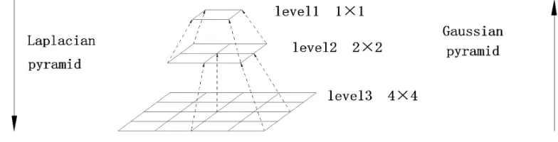
1. We construct a Gaussian pyramid G(I) = [I1, I2, …, In], here I1= Iand Inis N recursive applications of down(•) to I. The IN can be viewed as the Nthnumber of levels in the pyramid. In addition, the top level has to retain a certain size because the image has too few pixels to recover (we usually set N = 3 in pre-trained module). We initialize down-top levels with Gaussian kernel w and then let even lines be removed:

2 2

1 2 2

( , ) ( , ) (2 , 2 )

N N

m n

I i j w m n I  i m j n

 



 

2. The image LN(I) denotes Nth levels of Laplacian pyramid, which is make up of 2 adjacent levels in the Gaussian pyramid. Then we up-sample the smaller image with up(•) operator, so the image LN(I) sizes can be expressed as:

1 1

( ) ( ) ( ( )) ( )

N N N N N

L I G I up G  I I up I  (3)

3. Obviously, each level is corresponding to a scale image. As a low-frequency residual, the top level image can be equal with the Gaussian pyramid when GN(I) = LN(I), here GN(I) represents the N level in the Gaussian pyramid. The finest image in pre-trained module is calculated by combining Laplacian pyramid image with the backward recurrence, and the result IN can also be viewed as:

1

= ( )+ ( )

N N N

I up I  L I (4) Figure 2. Our architecture of the Advanced Generative Adversarial Network.

In summary, beginning with the coarsest level, we alternately up-sample and add particular scale image LN(I) from the following finer level. Finally, we can calculate a finest image in pre-trained module.

3.1.2. Convolutional skip-connections

The typical CNN algorithms have been proved to exhibit great advantages for SR tasks [33]. These CNN-based algorithms extract effective and robust features from LR information by convolutional layers, such as SRCNN, VDSR, DRRN. The convolution and ReLU operator can be viewed as:

( ) max( ,0)

f x  w x b (5)

However, some GAN methods are not successfully applied to image super-resolution. The authors of DCGAN utilize a cascade convolutional network to generate image representations. Although the above algorithm extracts the image features by convolutional neural network, the cascade architecture limits generator to learn deep semantic features. We argue that feature maps from intermediate layers may contain some latent information, which is crucial for image representations. Therefore, it is important for our generator to employ some convolutional skip-connections and then extract feature maps from intermediate layers, which effectively avoid deep semantic loss. The deployed convolutional skip-convolutions can be represented by the following in Figure 5. There are 5 blocks in the network. The 1st _{block can extract some coarse features. 3}

convolutional skip-connections (from 2nd _{block to 4}th _{block) are used to carry semantic information}

for generated images, the last convolutional layer generates synthesized images in the 5th _block.

The convolutional skip-connections effectively play a significant role in the forward propagation and backward propagation, respectively. On the one hand, each convolutional skip-connection

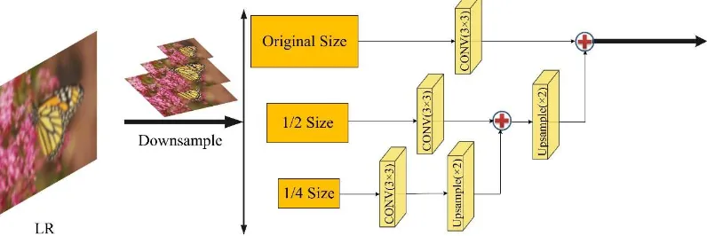
Figure 4. The Laplacian pyramid framework for our pre-trained module. It contains 3 convolutional layers with 3×3 filter kernels and 2 up-sample operators by a factor of 2.

introduces a convolutional layer compared with traditional skip-connections, which slightly adjusts the feature maps extracted during the forward propagation. On the other hand, our convolutional skip-connections alleviate gradient vanishing problem in the backward propagation because the gradient is passed directly by our convolutional skip-connections.

Specifically, we use small 3×3 kernels for convolutional layers inspired by Szegedy et al. [34] and the activation function ReLU as our 1st _{block. From 2}nd _{to 4}th _{blocks, a series of fractional-strided}

convolutions (FSC) are applied to all convolutional layers as proposed by Radford et al. Considering the batch normalization (BN) is usually utilized to counteract the internal covariate shift, [35] BN helps bridge between the fractional-strided convolutions and ParametricReLU. For activation function PReLU, the mathematical formulation can be expressed as:

PReLU( ) max( , 0)x  x amin(0, )x (6)

Where x denotes the input signal, and the parameter a is learnable for PReLU in negative part, which effectively alleviate “dead feature” in zero gradients [36]. In 5th _{block, the convolutional layer}

generates a plausible-looking image, with the goal of fooling a discriminative model D.

3.2. Discriminative network structure

For the discriminator, it improves constantly learning ability to distinguish between generated images or real images during the training procedure. As shown in Figure.2, our discriminative network is optimized in structure compared with traditional discriminator.

Specifically, we employ 10 convolutional layers with a size of 3×3 kernels. In order to obtain more context, the size of receptive field is increased by a factor of 2 from 64 to 512. Considering that the sizes are proportional to the layers, we follow the available framework of VGG19 network. Similar to the generator, there are 3 CBL modules in our discriminative network. Each CBL module contains convolutional layers, BN and LReLU. We also employ 2 convolutional skip-connections after each CBL module, which can obtain more high-frequency details to distinguish images. The convolutional layers are used to extract abundant features. The 512 results are followed by a dense layer and a flatten layer. These operations map each multi-dimensional input onto another one-dimensional vector. Then, the vectors are fed into fully connected layers to combine the features from previous layers. Finally, a sigmoid function with one node produces a probability for classification.

3.3. Perceptual loss function

A two-player minimax game proposed by Goodfellow et al. [9] has been proved to show hugely performance for loss functions. Firstly, the authors take noise z from distribution in generative model G over data x as an input variable pz(z). Secondly, they maps input z to data space G(z;θ) over the

generative network. During the training procedure, the generator has enough capacity to fool the discriminative model, in order to maximize the probability of discriminator to believe the fake samples from real images. The generative model G is trained to minimize log(1-D(G(z))). Thirdly, the discriminative model D improves constantly learning ability, and then distinguishes whether the images from the generator or from data distribution. Likewise, they maximize log(D(x)) for the discriminator. The value function for GAN are composed as follows:

~ ( ) ~ ( )

min max ( , ) [log ( )] [log(1 ( ( )))] = ( ) log ( ) ( ) log(1 ( ( )))

= ( ) log ( ) ( ) log(1 ( )

data z

x p x z p z

G D

data g

x x

data g

x

V D G D x D G z

p x D x dx p x D G z dx

p x D x dx p x D x dx

E

E







When G and D learn enough ability, they will reach a stationary point where both converge to a Nash equilibrium. Then the discriminative model D can be denoted in Equation (8) via G fixed.

#_{( )} ( ) ( ) ( ) data G data g p x D x

p x p x



When reach a stationary Nash equilibrium for pg=pdata, we use D x_G#( ) to denote D x( ) for simplicity and the Equation (9) can be reformulated as:

# # #

~ ~

~ ~

max ( , ) [log ( )] [log(1 ( ( )))] ( ) ( )

[log ] [log ]

( ) ( ) ( ) ( ) 0.5 ( ) 0.5 ( )

( ) ( ) ( ) ( ) ( ) log ( ) log

2 2

data z

data z

G G

x p z p

D

g data

x p z p

data g data g

g data

data g data g

data g

x x

V D G D x D G z

p x

p x

p x p x p x p x

p x

p x

p x p x p x p x

p x dx p x d

E

E

E

E





2log ( ) log ( ) log

2 2 2

1

2log 2 ( ( ) || ( )) 2

g data

data g data g

data g x x data g x p x p x

p x p x p x p x

p x dx p x dx

JSD p x p x

 

  

 





(9)

Here JSD(x||y) function is the abbreviation of Jensen-Shannon divergence between the generative model and data distribution [37]. However, the above loss function exhibits some limitations. For instance, the discriminator only focuses on whether the input is effectively distinguished (true or false), but there is no penalty for D when it misclassifies those fake samples. It is easy to cause the gradient vanishing problem where a saddle point may be found. Inspired by LSGAN, Mao et al. [38] adopt the least squares loss function for the discriminative model. Based on this observation, we employ energy-based regularization term as part of our loss function, to further improve the accuracy of the GAN. Since the center pixels in synthesized images are correlated with their neighbored ones, we argue that the generator can autonomously converge to reach point where is lower energy and more stable, under the conditions of regularization term.

In our adversarial network, generator and discriminator have different perceptional loss functions, respectively. There are 3 parts for generative loss function including content loss, adversarial loss and energy-based regularization. We define the content loss as MSE between synthesized images G(z) from the generator and the real images x from data distribution. The content loss ensures the G(z) as well as x is closer to perceptual similarity during the training. While having enough capacity to fool the discriminative model, it encourages the adversarial loss to get as small error (D(G(z))-1) as possible. Although each pixel xi in the images has more or less correlation with

neighbors of xj in the batch {x1, …, xn}, there are significant differences between pixels on the edge.

According to [39], we adopt the energy-based regularization E(zi,zj) to restrict the relationship

between center pixels and their neighbored ones generated by G. Our generative loss function can be formulated as follows:

2 2

1 2 3

,

( , ) || ( ) || || ( ( )) 1 || ( , )

G F F i j

i j

L x z n G z x n D G z  n



Here ||•||F denotes Frobenius norm, and the coefficient n1=1, n2=0.1, n3=0.1 in our experiment. The energy-based regularization

,

( , )_{i j}

i j

E z z



2 2

16 16

2 2

, 1 1

|| || ||1 | ||| ( , )= ( , ) exp( ) (1 ( , )) exp( )

2 2

i j i j

i j i j i j

i j i j

z z z z

E z z G z z G z z

a b

 

  

     





Where zi, zj represent the center pixel and its 16 connected pixels, respectively. G(zi, zj) denotes the gradient to reduce the error probability. In the Equation (11), we set a=1 and b=1 for simplicity. Note:

, = , =1

i j i j

i j

G z z if z z

G z z otherwise  

 

（ ）0

（ ） (12)

2 2

1 1

( , ( )) || ( ) 1|| || ( ( )) ||

2 2

D

L x G z  D x   D G z (13)

In summary, our perceptual loss function including generative and discriminative is significant for our network, by refining high-frequency details and correcting the errors between real images and generated images.

4. Experiments

In this section, we have demonstrated the excellent perceptual performance in our network. A large number of experimental results that we conduct are compared with state-of-the-art algorithms. There are 3 main sections: we first have a brief description about our algorithm. Then, we discuss some implementation details in our network structure, such as Laplacian pyramid, convolutional skip-connections and perceptual loss function. Compared with state-of-the-art algorithms, the last section has illustrated that the effective of our algorithm improves significantly based on public evaluation.

4.1. Experimental dataset and setting

The experiment of SR task is conducted to test on the benchmark datasets, including Set5, Set14, B100 and Urban100 [40]. Most of them are performed between LR and HR images on scale factor of ×2, ×3 and ×4, respectively. For fair comparison, the averaged peak signal to noise ratio (PSNR), structural similarity index (SSIM) and information fidelity criterion (IFC) are calculated for quantitative evaluation. In addition, the SR images for methods, which contain SRCNN, VDSR, DRRN and SRGAN, are captured by CMOS sensor in the real world and available online material.

Our network is conducted on a workstation with an Intel i7 6800K CPU, Linux operating system and two GeForce GTX1080 Ti GPUs. We train the 400 thousand images from the ImageNet dataset, which is different for the testing sets.

4.2. Implementation details

In order to rich the diversity of training samples, flipping and rotation techniques are introduced into a large database. For example, we rotate image by 0°, 90°, 180° or 270° to generate different directions. Then, we randomly flip between horizontal or vertical images. Additionally, there are 4 different scales including ×0.9, ×0.8, ×0.7 and ×0.6 for training images to enlarge the multi-scale samples.

4.2.1 Laplacian pyramid performance

Decreasing by a factor of 1/2 from original size to 1/4 size in the Laplacian pyramid framework, we obtain the LR images by using down-sample operator on the HR images. A multi-scale Gaussian pyramid G(I) = [I1, I2, I3] has been built. As shown in Figure 4, we use bicubic kernel (3×3) with up-sampling operation to match the size of upper layer. Specifically, we first up-sample the 1/4 size image by a factor of 2, and connect to the 1/2 size image. Then, we up-sample the 1/2 size with ×2 factor to match the original size image. The up-sample operator on the small image (1/4 size, 1/2 size) is from Equation (3). All path inputs, which have the same size, are fused into a Laplacian pyramid image.

Table 1. Comparison with different sized inputs on B100 and Urban100 with ×2

Inputs

B100

Urban100

Average PSNR(dB)

Average PSNR(dB)

Original size

32.30

30.79

Original size + 1/2 size

32.38

30.88

Original size + 1/2 size + 1/4 size

32.41

30.93

4.2.2 Convolutional skip-connections performance

Note that the feature maps from intermediate layers may contain some latent information in Figure 5, we design 3 groups to compare with different numbers on convolutional skip-connections (CSC) and show visual comparisons on Set14.

Table 2. Comparison with different convolutional skip connections in each input

Inputs

1st

CSC (Red)

2nd

CSC (Blue) 3rd CSC (Green)

(a)

√

(b)

√

√

(c)

√

√

√

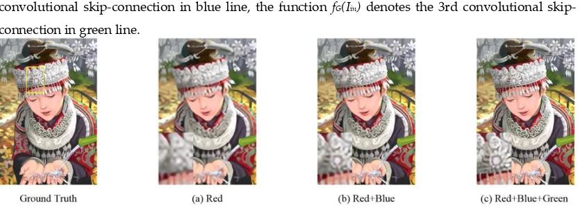
As shown in Table.2, we employ 3 convolutional skip-connections based on our network to reconstruct the HR image as accurately as possible. In other word, the red line represents 1st convolutional skip-connection to refine feature maps. Similarly, the blue line and green line denote 2nd convolutional skip-connection and 3rd convolutional skip-connection, respectively. There are 3 convolutional skip-connections to construct a parallel module, which can be expressed as:

( ) ( ) ( ) ( )

out in R in B in G in

I FBP I f I f I f I (14) Here, Iin, Iout denote input image and output image, respectively. The function FBP is made up of FSC, BN and PReLU and then we use FBP(Iin) represents a cascade network. In addition, the function fR(Iin) denotes the 1st convolutional skip-connection in red line, the function fB(Iin) represents the 2nd convolutional skip-connection in blue line, the function fG(Iin) denotes the 3rd convolutional skip-connection in green line.

As shown in Figure.6, the image generated by 3 CSC has richer details compared other 2 groups. So, our parallel module including 3 CSC reconstructs HR images by carrying much semantic information and refining feature maps.(a) the generative network has only a red convolutional skip-connections. (b) there are 2 convolutional skip-connections including red and blue in generative

network. (c) our generative network is a parallel architecture, which contains red, blue and green convolutional skip-connections.

4.2.3 Perceptual loss function performance

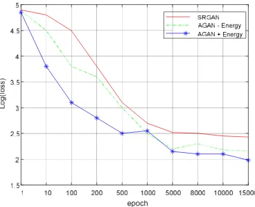
As stated in section 3.3, the implementation of perceptual loss function can be trained to alleviate loss through the adversarial network. In our experiment, we evaluate the performance of 3 loss functions, the loss function of SRGAN, AGAN without energy-based regularization, and AGAN with energy-based regularization. The value of three loss functions with the number of epochs are shown in the Figure.7. It is clear that our network is better quality than others. When the epochs reach 5000, the loss caused by generator and discriminator have been stable. In other word, G has learned capacity enough to generate fake images, and D can also provide real-time feedback for G, which is beneficial to tune hyper parameters. On the one hand, AGAN has smaller loss compared with SRGAN, which accelerates convergence speed. On the other hand, the energy-based regularization overcomes overfitting effectively and makes the generated images have robust details.

Although most GAN algorithms have momentum during training progress, we use Adaptive Moment Estimation (Adam) for all hyper parameters [41]. This method not only stores the average exponential decay in AdaDelta but keeps the average exponential decay from gradient M(t). It is similar to momentum method.

*

1

( ) ( )

1 t

M t M t

 



*

2

( ) ( )

1 t

V t V t

 



Here M(t), V(t) are the gradient of first-order moment estimation and second-order moment estimation. We set the momentum β1=0.9 and β2=0.999. The variable M*(t) and V*(t) can be used as unbiased estimation to correct M(t), V(t).

4.3. Comparisons with the state-of-the-arts

provided in Table 3 and Table 4. These experimental results shown that AGAN achieves great performance in terms of average PSNR, SSIM, and IFC metrics.

4.3.1 Compare with Synthetic Data

For benchmark, we choose datasets “Set5” and “Set14” as synthetic data. Considering that most of SR algorithms can achieve great result, we use image quality metrics including PSNR and SSIM to compare performance on ×2, ×3 and ×4 SR. In addition, we employ bicubic interpolation on the color components and all networks are applied to luminance channel. Both inputs and outputs have the same size.

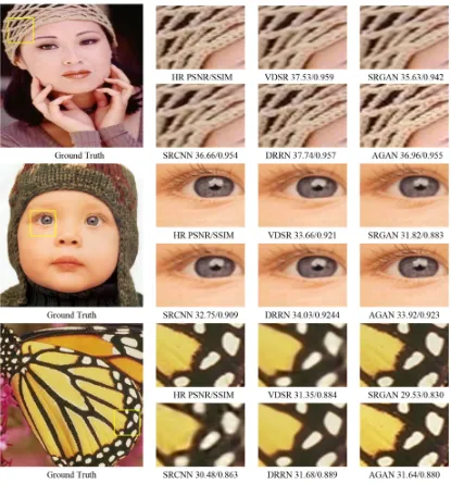
As shown in Figure 8, we partially enlarge the woman’s headwear, baby’s eye and butterfly’s wings. It can be found that the edge-preserving generated by SRCNN algorithm is significantly blurred. Further, DRRN can achieve higher PSNR and SSIM than other algorithms. However, the results generated by GAN have clear effects from visual perception. SRGAN and our algorithms can learn more high-frequency information, which is conducive to improve the image quality.

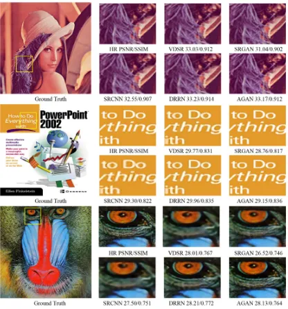
To further illustrate the effects of our algorithm, we select Set14 database (such as “lenna”, “ppt3” and “baboon”) for experimental comparison. In the first row of Figure 9, we find that AGAN is able to produce clear hair and have sharper details. As shown in the second row of Figure 9, the “ppt3” image by SRCNN method has blurred text. DRRN algorithm exhibits an improvement compared to SRCNN and VDSR, but it is lacking high-frequency details. Different from the other 4 approaches, our algorithm is closer to ground truth image in the third row.

4.3.2 Compare with Real-world Images

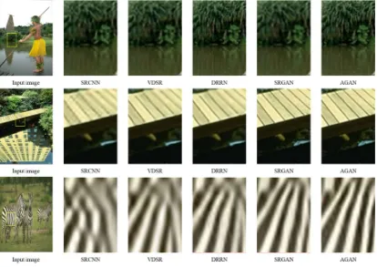
In order to demonstrate an application of SR tasks, several visual examples from datasets “B100” and “Urban100” are measure on real-world images. In these cases, neither the down-sample operator nor the ground truth images are available. Figure 10 and Figure 11 show the visual results between our algorithm and other methods.

It can be observed from Figure 10 and Figure 11, our proposed AGAN outperforms other 4 methods in both details and sharpness. For example, VDSR method tends to produce blurry results (image “101087” on B100), whose textures are unnatural and have undesired noise. Our method can generate sharper and more natural grass textures.

Besides, AGAN is capable of making more detailed structures in building (image “img077” on Urban100) while other algorithms either fail to generate enough details (SRGAN) or introduce unpleasing textures (DRRN). Meanwhile, previous methods usually add artifacts to the images, but our algorithm gets rid of these artifacts and more sensitive to visual perception.

Table 3. Benchmark results. Average PSNR, SSIM and IFC on datasets for comparison, increasing by a factor of 2, 3 and 4.

As reported in visual examples, the generative HR images not only express more pleasing effect, but also have much sharp and vivid contours under the deep supervision of discriminator. In Table 3, Red color denotes the best performance of proposed methods and blue color indicates the best performance of previous methods. Our algorithm achieves a greater score rely on novel network structure. It is crucial for the plausible results based on 4 benchmark datasets, using Laplacian pyramid and convolutional skip-connections. In addition, energy-based regularization strategy, which can capture high-frequency details, has been adopted in our loss function.

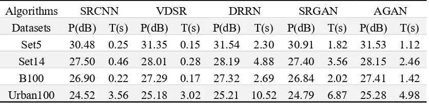
Table 4. The average PSNR (dB) and test time (s) for magnification factor ×4 are compared

Algorithms

SRCNN

VDSR

DRRN

SRGAN

AGAN

Datasets

P(dB) T(s) P(dB) T(s) P(dB) T(s) P(dB) T(s) P(dB) T(s)

Set5

30.48 0.25 31.35 0.15 31.54 2.30 30.91 1.82 31.53 1.12

Set14

27.50 0.46 28.01 0.28 28.19 4.88 27.40 3.56 28.15 2.46

B100

26.90 0.22 27.29 0.17 27.32 2.69 26.84 2.02 27.41 1.42

Urban100 24.52 3.56 25.18 3.02 25.21 10.52 24.79 6.87 25.28 4.98

Datasets Scale SRCNN VDSR DRRN SRGAN AGAN

Ｘ２ 36.66/0.9542/8.04 37.53/0.9587/8.19 37.74/0.9571/8.67 35.63/0.9418/8.23 36.96/0.9553/8.43 Ｘ３ 32.75/0.9090/4.66 33.66/0.9213/5.22 34.03/0.9244/5.40 31.82/0.8826/4.69 33.92/0.9234/5.47

Ｘ４ 30.48/0.8628/3.00 31.35/0.8838/3.50 31.68/0.8888/3.70 29.53/0.8304/3.12 31.64/0.8798/3.76

Ｘ２ 32.45/0.9067/7.79 33.03/0.9124/7.88 33.23/0.9136/8.32 31.04/0.9018/7.83 33.17/0.9123/8.25 Ｘ３ 29.30/0.8215/4.34 29.77/0.8314/4.73 29.96/0.8349/4.88 28.76/0.8171/4.82 29.25/0.8324/4.99

Ｘ４ 27.50/0.7513/2.75 28.01/0.7674/3.07 28.21/0.7720/3.25 26.52/0.7470/3.17 28.13/0.7602/3.29

Ｘ２ 31.36/0.8879/7.24 31.90/0.8960/7.17 32.05./0.8973/7.70 30.85/0.8342/7.32 31.98/0.8921/7.74

Ｘ３ 28.41/0.7863/3.37 28.82/0.7976/3.94 28.95/0.8004/4.21 27.80/0.7363/4.04 28.89/0.8005/4.35

Ｘ４ 26.90/0.7101/2.41 27.29/0.7251/2.63 27.38/0.7284/2.77 25.43/0.6633/2.59 27.11/0.7186/2.82

Ｘ２ 29.50/0.8946/8.00 30.76/0.9140/8.27 31.23/0.9188/8.92 29.75/0.9033/8.33 31.39/0.9202/9.01

Ｘ３ 26.24/0.7989/4.58 27.14/0.8279/5.19 27.53/0.8378/5.47 27.15/0.8076/5.32 27.61/0.8441/5.54

Ｘ４ 24.52/0.7221/2.96 25.18/0.7524/3.41 25.44/0.7638/3.68 25.34/0.7310/3.51 25.40/0.7639/3.77

B100

Urban100 Set5

Set14

There is a trade-off between the speed (time) and performance (PSNR) by a factor of 4 on datasets, including Set5, Set14, B100 and Urban100. All algorithms are trained on the ImageNet dataset for a fair comparison. In Table 4, we find that our network solves real-time SR task while having a good performance. For example, our algorithm achieves a higher 0.6 dB than SRGAN in average PSNR when has the same test time. Meanwhile, AGAN also is a fast method which is 2 times faster than DRRN while reaching stable point.

5. Conclusions

As the images captured by CMOS sensor are not exhibited effectively for high-frequency details, we propose a novel super-resolution algorithm based on Advanced Generative Adversarial Network (AGAN). In order to better learn semantic features and generate image representations, the Laplacian pyramid and convolutional skip-convolutions frameworks have been accepted. It is significant for generative model to generate a plausible-looking image. In addition, we also present perceptual loss function, which can further refine high-frequency details. Quantitative and qualitative evaluations have been demonstrated that AGAN algorithm performs better than previous GAN algorithms for super-resolution task. Experimental results also show that the proposed method can fully take advantage of CNN to improve the image quality by CMOS sensor. Nevertheless, our algorithm has some limitations, like producing some nonsensical outputs and unstable to train. These problems will be studied in our future work.

Author Contributions: Shiping Wang designed the research and wrote the paper; Linyuan He contributed the idea; Chen Wang performed the experiments; Duyan Bi revisited and supervised the paper.

Acknowledgments: This work was supported by the National Natural Science Foundation of China, under Grants 61701524 and 61372167. Thanks to the anonymous reviewers for their valuable suggestions.

Conflicts of Interest: The authors declare no conflict of interest.

References

1. Kim, D.; Song, M.; Choe, B.; Kim, S. A Multi-Resolution Mode CMOS Image Sensor with a Novel Two-Step Single-Slope ADC for Intelligent Surveillance Systems. Sensors 2017, 17, 1497-1509.

2. Dong, C.; Loy, C.; He, K.; Tang, X. Image Super-Resolution Using Deep Convolutional Networks. TPAMI 2015, 38, 295-307.

3. Dong, C.; Loy, C.; He, K.; Tang, X. Learning a Deep Convolutional Network for Image Super-Resolution. In Proceedings of the 2014 European Conference on Computer Vision, Zurich, Switzerland, 6 September-12 September; pp. 184-189.

4. Kim, J; Lee, J.J; Lee, K. M. Accurate Image Super-Resolution Using Very Deep Convolutional Networks. In Proceedings of the 2016 Computer Vision and Pattern Recognition, Las Vegas, USA, 26 June-1 July; pp. 1646-1654.

5. Lai, W. S; Huang, J. B; Ahuja, N; Yang, M. Deep Laplacian Pyramid Networks for Fast and Accurate Super-Resolution. In Proceedings of the 2017 Computer Vision and Pattern Recognition, Hawaii, USA, 21 July-26 July; pp. 1548-1556.

6. Tai, Y; Yang, J; Liu, X. M. Image Super-Resolution via Deep Recursive Residual Network. In Proceedings of the 2017 Computer Vision and Pattern Recognition, Hawaii, USA, 21 July-26 July; pp. 1028-1036. 7. Hong Y; Hwang U; Yoo J. How Generative Adversarial Networks and Their Variants Work: An Overview

of GAN. 2017.

8. Doersch, C. Tutorial on Variational Autoencoders. arXiv 2016, arXiv:1606.05908.

9. Goodfellow, I; Pouget-Abadie, J; Mirza, M; Xu, B; Farley, D. Generative Adversarial Nets. In Proceedings of 2014 Neural Information Processing Systems, Montreal, Canada, 8 December-13 December; pp. 2672-2680.

10. Lucic M; Kurach K; Michalski M. Are GANs Created Equal? A Large-Scale Study[J]. 2017.

12. Blu. T; Thevenaz. P; Unser. M; Linear interpolation revitalized. TIP 2004, 13, 710-719.

13. Timofte, R; Smet, V; Gool, V.G. A+: Adjusted Anchored Neighborhood Regression for Fast Super-resolution. In ACCV, 2014.

14. Wang, Z; Liu, D; Yang, J; Han, W; Huang, T. Deep Networks for Image Super-resolution with Sparse Prior. In ICCV, 2015.

15. Timofte, R; Agustsson, E; Yang, H. Ntire 2017 Challenge on Single Image Super-resolution. In CVPR 2017. 16. Timofte R ; De V ; Gool L V . Anchored Neighborhood Regression for Fast Example-Based Super-Resolution

2013 IEEE International Conference on Computer Vision (ICCV). IEEE Computer Society, 2013.

17. Yang J; Xiao B W; Yan J J. Multi-scale Learning Based Data Processing Mechanism for Wireless Body Area Network. Science Technology & Engineering, 2018.

18. He K; Zhang X; Ren S. Delving Deep into Rectifiers: Surpassing Human-Level Performance on ImageNet Classification. 2015:1026-1034.

19. Kim K I; Kwon Y. Single-image super-resolution using sparse regression and natural image prior.[J]. IEEE Transactions on Pattern Analysis & Machine Intelligence, 2010, 32(6):1127.

20. Schulter S; Leistner C; Bischof H . Fast and accurate image upscaling with super-resolution forests 2015 IEEE Conference on Computer Vision and Pattern Recognition (CVPR). IEEE Computer Society, 2015. 21. He H; Siu W C. Single image super-resolution using Gaussian process regression Computer Vision and

Pattern Recognition. IEEE, 2011:449-456.

22. Dai D; Timofte R; Gool L V . Jointly Optimized Regressors for Image Super-resolution Computer Graphics Forum. 2015.

23. Zhu, J.M; Park, T; Isola, P. Unpaired Image-to-Image Translation using Cycle-Consistent Adversarial Networks. In Proceedings of the 2017 International Conference on Computer Vision, Venice, Italy, 22 October-29 October; pp. 1058-1079.

24. Shi, W; Caballero, J; Huszar, F; Totz, J; Z. Wang. Real-time Single Image and Video Super-resolution Using an Efficient Sub-pixel Convolutional Neural Network. In CVPR, 2016.

25. Guosheng Lin; Chunhua Shen; Anton van den Hengel; Ian Reid. Exploring Context with Deep Structured models for Semantic Segmentation. IEEE Transactions on Pattern Analysis and Machine Intelligence, 2017, 6, 864-880.

26. Radford; Alec; Metz; Luke; Chintala; Soumith. Unsupervised Representation Learning with Deep Convolutional Generative Adversarial Networks. Computer Science, 2015.

27. Ledig C; Wang Z; Shi W. Photo-Realistic Single Image Super-Resolution Using a Generative Adversarial Network. Computer Vision and Pattern Recognition. IEEE, 2017:105-114.

28. Kim, J; Lee, J.J; Lee, K. M. Deeply-Recursive Convolutional Network for Image Super-Resolution. In Proceedings of the 2016 Computer Vision and Pattern Recognition, Las Vegas, USA, 26 June-1 July; pp. 1543-1551.

29. Dong C; Chen C L; Tang X. Accelerating the Super-Resolution Convolutional Neural Network. 2016:391-407.

30. Chen X; Duan Y; Houthooft R. InfoGAN: Interpretable Representation Learning by Information Maximizing Generative Adversarial Nets. 2016.

31. Yang, J.; Wright, J.; Huang, T.; Ma, T. Image Super-resolution as Sparse Representation of Raw Image Patches. Proceedings of the 2012 Computer Vision and Pattern Recognition, Rhode Island, USA, 16 June-21 June; pp. 372-380.

32. Zeyde, R.; Elad, M.; Protter, M. On Single Image Scale-up Using Sparse-representations. Curves and Surfaces 2012; pp. 711–730.

33. Zhang, K; Gao, X; Tao, D; Li. X. Multi-scale Dictionary for Single Image Super-resolution. In Proceedings of the 2012 Computer Vision and Pattern Recognition, Rhode Island, USA, 16 June-21 June; pp. 1114–1121. 34. Szegedy C; Ioffe S; Vanhoucke V. Inception-v4, Inception-ResNet and the Impact of Residual Connections

on Learning. 2016.

35. Chen, L.C; Papandreou, G; Kokkinos, I; Murphy, K; Yuille, A. Semantic Image Segmentation with Deep Convolutional Nets. IEEE Transactions on Pattern Analysis and Machine Intelligence, 2016, 4, 566-582. 36. Bevilacqua, C.M; Roumy, A; Morel, M. Low Complexity Single-image Super-resolution Based on

Nonnegative Neighbor Embedding. In BMVC. 2012.

38. Mao X; Li Q; Xie H. Least Squares Generative Adversarial Networks. 2016.

39. Martin, D; Fowlkes, C; Tal, D; Malik, J. A Database of Human Segmented Natural Images and Its Application to Evaluating Segmentation Algorithms and Measuring Ecological Statistics. In ICCV, 2001. 40. Kingma D , Ba J . Adam: A Method for Stochastic Optimization. Computer Science, 2014.