Approximate methods for dynamic portfolio allocation under transaction costs

(1)

Western University Western University

Scholarship@Western

Electronic Thesis and Dissertation Repository

9-7-2012 12:00 AM

Approximate methods for dynamic portfolio allocation under

transaction costs

Nabeel Butt

The University of Western Ontario

Supervisor Dr Matt Davison

The University of Western Ontario Co-Supervisor Dr Greg Reid

The University of Western Ontario

Graduate Program in Applied Mathematics

A thesis submitted in partial fulfillment of the requirements for the degree in Doctor of Philosophy

Follow this and additional works at: https://ir.lib.uwo.ca/etd

Part of the Control Theory Commons, Dynamic Systems Commons, Numerical Analysis and Computation Commons, Portfolio and Security Analysis Commons, Probability Commons, and the

Statistical Models Commons

Recommended Citation Recommended Citation

Butt, Nabeel, "Approximate methods for dynamic portfolio allocation under transaction costs" (2012). Electronic Thesis and Dissertation Repository. 932.

https://ir.lib.uwo.ca/etd/932

This Dissertation/Thesis is brought to you for free and open access by Scholarship@Western. It has been accepted for inclusion in Electronic Thesis and Dissertation Repository by an authorized administrator of

(2)

APPROXIMATE METHODS FOR DYNAMIC PORTFOLIO ALLOCATION

UNDER TRANSACTION COSTS

(Spine title: Dynamic Portfolio Allocation under transaction costs )

(Thesis format: Monograph)

by

Nabeel Butt

Graduate Program in Applied Mathematics

A thesis submitted in partial fulfillment

of the requirements for the degree of

Doctor of Philosophy

The School of Graduate and Postdoctoral Studies

The University of Western Ontario

London, Ontario, Canada

c

(3)

THE UNIVERSITY OF WESTERN ONTARIO

School of Graduate and Postdoctoral Studies

CERTIFICATE OF EXAMINATION

Supervisor:

. . . . Dr. Matt Davison

Joint Supervisor:

. . . . Dr. Greg Reid

Supervisory Committee:

. . . . Dr. Adam Metzler

Examiners:

. . . . Dr. Adam Metzler

. . . . Dr. Ian Mcleod

. . . . Dr. Matt Thompson

. . . . Dr. Mark Reesor

The thesis by

Nabeel Butt

entitled:

APPROXIMATE METHODS FOR DYNAMIC PORTFOLIO ALLOCATION UNDER TRANSACTION COSTS

is accepted in partial fulfillment of the requirements for the degree of

Doctor of Philosophy

. . . . Date

. . . .

Chair of the Thesis Examination Board

(4)

Acknowledgments

I would like to start by expressing my deepest gratitude towards God for all His help and support all along. Next I thank my beloved parents for their efforts in helping me get the best education possible. I would also like to thank all my thesis examiners for their insightful comments leading to a much improved version of the thesis.

My PhD years at UWO were some of the best years of my life. My primary Phd supervisor Dr Matt Davison was an ever present support and a great source of guidance. Matt was very helpful in all our meetings and gave me complete freedom to pursue novel ideas. It was Matt who initially directed me towards a MITACS 2008 industrial problem solving workshop. Many of the ideas in the thesis were inspired by different aspects of the hedge fund problem the workshop involved. My co-supervisor Dr Greg Reid was a great source of advice and sparked my interest in Homotopy methods in applied mathematics. Greg also helped me develop an interest in experimental mathematics.

Last but not the least I would like to thank my imaginary friend Mathematica for all its support ! :-)

(5)

Abstract

The thesis provides simple and intuitive lattice based algorithms for solving dynamic port-folio allocation problems under transaction costs. The early part of the thesis concentrates upon developing a toolbox based on discrete probability approximations. The discrete ap-proximations are shown to provide a reasonable approximation for most popular transaction cost models in the academic literature. The tool, once forged, is implemented in the powerful Mathematica based parallel computing environment. In the second part of the thesis we pro-vide applications of our framework to real world problems. We show re-balancing portfolios is more valuable in an investment environment where the growth and volatility of risky assets is non-constant over the time horizon. We also provide a framework for modeling random transaction costs and compute the loss of expected utility of an investor faced with random transaction costs. Approximate methods are provided to solve portfolio constraints such as portfolio insurance and draw-down. Finally, we also highlight a lattice based framework for pairs trading.

Keywords: Portfolio Allocation, Transaction costs

(6)

List of Figures

2.1 Static versus Dynamic investor. A static investor re-balances only once while a dynamic investor re-balances at nodes inside. . . 5

2.2 Merton line under no-transaction cost with parameters m = 0.14, ω = 0.05.

Wheremis the drift for the risky asset andωis the risk-free rate. . . 7 2.3 Re-balancing toMertonline for CRRA or log-utility. The line is constant with

respect to time. . . 8 2.4 No-transaction boundaries over a finite horizon for CRRA or log-utility. When

the investor moves closer to terminal time the no-transaction region widens. . . 9 2.5 Controlled risky fraction over a finite horizon for CRRA or log-utility under

transaction costs. Risky fraction is controlled via transaction so that it never falls outside the buy-side and sell-side boundaries. . . 10 2.6 Lattice solution methodology for Bermudan option. . . 15

2.7 Lattice solution methodology for dynamic portfolio problem. . . 16

3.1 Risk-adjusted value of re-balancing portfolios with parameters T = 1, ω = 0.07, λ= µ=0.005,s= eω∆T,m=0.14, σ=0.3. WhereT is the time horizon for investment,ωis the continuous time risk-free rate, (λ, µ) are transaction cost factors, sis the risk free growth over the interval,mis the drift for continuous time GBM andσis the volatility for the continuous time GBM. The continuous time GBM implies a risky growth for the risky asset over the interval∆T. . . . 24

3.2 Discrete time trading model. The dynamic investor has the option to re-balance or not to re-balance at a time node. The risky asset grows over the re-balancing period and so the fraction of wealth in the risky asset changes. . . 25

3.3 A possible piecewise linear function for transaction costs. Transaction costs are a function of the amount traded. . . 26

3.4 A possible no-transaction region in state variable space. For Log and CRRA utility if the fraction of wealth in risky asset goes out of the boundaries the risky fraction is brought inside the boundary [28]. . . 27

3.5 A no-transaction region for transfer of wealth model between three assets where ♣ denotes no-transaction. Parameters intentionally not supplied. Horizontal axis is the fraction of wealth in first risky asset and vertical axis is the fraction of wealth in second risky asset. . . 29 3.6 Approximation with five points. Choosing statistical features of the target

prob-ability model for approximation. . . 32

(12)

3.7 No transaction region boundaries shifting monotonically outwards as investors moves closer to terminal time for last, second and third last stage parameters are: V = 0.5,T = 0.1,N = 3, ω = 0.05,s = eω∆T,_m = ₀.₁₄, σ = ₀._8. _N _is

number of re-balancing nodes andsis the risky free growth over the interval.V

is the co-efficient of risk aversion in the CRAA utility. Alsom andσ are the parameters of the continuous time GBM and risky growth discrete probabil-ity approximation is constructed as we will discuss later in section 3.8.3 and 3.9.WhereT is the time horizon for investment,ωis the continuous time risk-free rate, (λ, µ) are transaction cost factors, s is the risk free growth over the interval,mis the drift for continuous time GBM andσis the volatility for the continuous time GBM. The continuous time GBM implies a risky growth for the risky asset over the interval∆T. . . 35 3.8 No transaction region in 2-D at time t=0 CRRA utility. Parameters not

inten-tionally given. Purpose is to provide a visual depiction. No-transaction region is a parallelogram marked with ♥. 38 3.9 A discrete probability approximation approximation in 1-D. HererT say risky

growth over an interval is variable being approximated. . . 39 3.10 Illustrating discrete probability approximation construction in 2-D for

corre-lated variables. . . 40 3.11 Illustrating discrete probability approximation construction in 3-D for

corre-lated variables. . . 41 3.12 Convergence in value for CRRA utility for a discrete probability approximation

approximation varying N = 5,10, ...,30 and parameters:T = 1, ω = 0.1,s = eω∆T,m= 0.24, σ= 1, λ= µ= 0.01,V =0.5. WhereT is the time horizon for investment, N is the number of re-balancing nodes. ω is the continuous time risk-free rate, (λ, µ) are transaction cost factors, s is the risk free growth over the interval,mis the drift for continuous time GBM andσis the volatility for the continuous time GBM. The continuous time GBM implies a risky growth for the risky asset over the interval∆T. . . 43 3.13 Convergence in value for log-utility for a discrete probability approximation

approximation varying N = 5,10, ...,30 and parameters:T = 1, ω = 0.1,s = eω∆T,_m = ₀.₁₄, σ = ₀.₃, λ = µ = ₀._{01. Where} _T _{is the time horizon for}

investment, N is the number of re-balancing nodes. ω is the continuous time risk-free rate, (λ, µ) are transaction cost factors, s is the risk free growth over the interval,mis the drift for continuous time GBM andσis the volatility for the continuous time GBM. The continuous time GBM implies a risky growth for the risky asset over the interval∆T. . . 44 3.14 Deformation solution by varying γ` = 1₅,₁₀1,₁₅1,₂₀1 for efficient frontier for a

jump diffusion problem with parametersT =1,N =4, ω= 0.07,s= eω∆T,m=

0.14, σ = 0.3, θ = 0.1, δ = 0.05. WhereT is the time horizon for investment,

N is the number of re-balancing nodes. ωis the continuous time risk-free rate, (λ, µ) are transaction cost factors, sis the risk free growth over the interval,m

is the drift for continuous time GBM andσis the volatility for the continuous time GBM. The continuous time GBM implies a risky growth for the risky asset over the interval∆T. γ`is the deformation parameter. . . 46

(13)

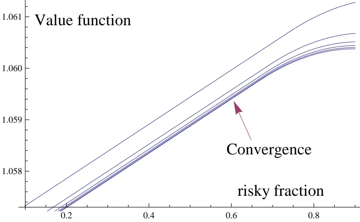
3.15 Deformation solution of value function with log-utility at t = 0 by varying

γ` = 1₅, ...,₃₀1 and parameters T = 1,N = 4, ω = 0.1, λ = µ = 0.01,s = eω∆T,_m = ₀.₁₄, σ= ₀._{3. Where}_T _{is the time horizon for investment,} _N _{is the}

number of re-balancing nodes.ωis the continuous time risk-free rate, (λ, µ) are transaction cost factors,sis the risk free growth over the interval,mis the drift for continuous time GBM andσis the volatility for the continuous time GBM. The continuous time GBM implies a risky growth for the risky asset over the interval∆T. γ` is the deformation parameter. . . 47

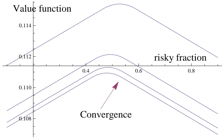
3.16 Deformation solution of value function with CRRA utility att = 0 by varying

γ` = 1₅, ...,₃₀1 and parameters T = 1,N = 4, ω = 0.1, λ = µ = 0.01,s = eω∆T,m= 0.14, σ= 0.3,V = 0.5. WhereT is the time horizon for investment,

is the drift for continuous time GBM andσis the volatility for the continuous time GBM. The continuous time GBM implies a risky growth for the risky asset over the interval∆T. γ`is the deformation parameter. . . 48

3.17 Deformation solution of value function with log-utility and jump diffusion model at t = 0 by varyingγ` = 1₅, ...,₂₀1 and parameters: T = 1,N = 4, ω =

0.1, λ = µ = 0.01,s = eω∆T,m = 0.14, σ = 0.6, θ = 0.1, δ= 0.05. WhereT is the time horizon for investment, N is the number of re-balancing nodes. ωis the continuous time risk-free rate, (λ, µ) are transaction cost factors,sis the risk free growth over the interval,mis the drift for continuous time GBM andσis the volatility for the continuous time GBM. The continuous time GBM implies a risky growth for the risky asset over the interval∆T. γ` is the deformation

parameter. . . 49

3.18 Deformation solution of value function with CRRA utility and jump diffusion model at t = 0 by varyingγ` = 1₅, ...,₂₀1 and parameters: T = 1,N = 4, ω =

0.1, λ = µ = 0.01,s = eω∆T,m = 0.14, σ = 0.3, θ = 0.1, δ = 0.05,V = 0.5. WhereT is the time horizon for investment, N is the number of re-balancing nodes.ωis the continuous time risk-free rate, (λ, µ) are transaction cost factors,

s is the risk free growth over the interval, m is the drift for continuous time GBM and σ is the volatility for the continuous time GBM. The continuous time GBM implies a risky growth for the risky asset over the interval∆T. γ`is

the deformation parameter. . . 50

3.19 Finite time solution to the CARA utility problem:T = 5,N =50, ω=0.05,s= eω,m = 0.18, σ = 0.4, λ = µ = 0.01,z = 0.01 using a risky growth discrete probability approximation with 15 branches using a deformation parameter=₁₅1. WhereT is the time horizon for investment, N is the number of re-balancing nodes.ωis the continuous time risk-free rate, (λ, µ) are transaction cost factors,

s is the risk free growth over the interval, m is the drift for continuous time GBM and σ is the volatility for the continuous time GBM. The continuous time GBM implies a risky growth for the risky asset over the interval∆T. γ`is

the deformation parameter. . . 52

(14)

3.20 Terminal wealth distribution for an investor maximizing E[Pr(WN > K)] with

parameters: T = 0.5,N = 5, ω = 0.05,s = eω∆T,m = 0.12, σ = 0.5, λ =

µ = 0.001,K = 0.208. Where T is the time horizon for investment, N is the number of re-balancing nodes.ωis the continuous time risk-free rate, (λ, µ) are transaction cost factors,sis the risk free growth over the interval,mis the drift for continuous time GBM andσis the volatility for the continuous time GBM. The continuous time GBM implies a risky growth for the risky asset over the interval∆T. γ` is the deformation parameter. . . 53

3.21 Terminal wealth distribution for an investor minimizing variability of wealth around a target level so that we minimizeE[(WN −b)2] with parameters: T =

0.5,N = 5, ω = 0.05,s = eω∆T,m = 0.12, σ = 0.5, λ = µ = 0.001,b = 0.4. WhereT is the time horizon for investment, N is the number of re-balancing nodes. Herebis the target level,ωis the continuous time risk-free rate, (λ, µ) are transaction cost factors, sis the risk free growth over the interval,mis the drift for continuous time GBM andσis the volatility for the continuous time GBM. The continuous time GBM implies a risky growth for the risky asset over the interval∆T. γ`is the deformation parameter. . . 54

3.22 Terminal wealth distribution for an investor maximizing E[W

V N

V ] with

param-eters: T = 0.5,N = 5, ω = 0.05,s = eω∆T,_m = ₀.₁₂, σ = ₀.₅, λ = µ =

0.001,V = 0.5. Where T is the time horizon for investment, N is the number of re-balancing nodes. ω is the continuous time risk-free rate, (λ, µ) are trans-action cost factors,sis the risk free growth over the interval,mis the drift for continuous time GBM and σ is the volatility for the continuous time GBM. The continuous time GBM implies a risky growth for the risky asset over the interval∆T. γ` is the deformation parameter. . . 55

3.23 Terminal wealth distribution for an investor maximizing E[W

V1

N

V1 +

W_NV2 V2 ] with parameters: T = 0.5,N = 5, ω = 0.05,s = eω∆T,_m = ₀.₁₂, σ = ₀.₅, λ = µ =

0.001,V1 = 1₃,V1 = 2₃. Where T is the time horizon for investment, N is the

number of re-balancing nodes.ωis the continuous time risk-free rate, (λ, µ) are transaction cost factors,sis the risk free growth over the interval,mis the drift for continuous time GBM andσis the volatility for the continuous time GBM. The continuous time GBM implies a risky growth for the risky asset over the interval∆T. γ` is the deformation parameter. . . 55

3.24 Variation of value function at time 0 with re-balancing frequency N for some choice of parameters:T = 1, ω= 0.05, λ = µ = 0.01,s = eω∆T,m = 0.14, σ = 0.7. Where T is the time horizon for investment, N is the number of re-balancing nodes. ω is the continuous time risk-free rate, (λ, µ) are transac-tion cost factors, sis the risk free growth over the interval, m is the drift for continuous time GBM and σ is the volatility for the continuous time GBM. The continuous time GBM implies a risky growth for the risky asset over the interval∆T. γ` is the deformation parameter. . . 56

(15)

3.25 Variation of value function at time 0 with re-balancing frequencyN with port-folio management fee for some choice of parameters:T = 1, ω = 0.07, λ =

µ = 0.001,s = eω∆T,_m = ₀.₁₈₂, σ = ₀._{4. Where}_T _{is the time horizon for}

investment, N is the number of re-balancing nodes. ω is the continuous time risk-free rate, (λ, µ) are transaction cost factors, s is the risk free growth over the interval,mis the drift for continuous time GBM andσis the volatility for the continuous time GBM. The continuous time GBM implies a risky growth for the risky asset over the interval∆T. γ`is the deformation parameter. . . 57

3.26 Variation of value function at time 0 with re-balancing frequencyN with port-folio management fee when investoralwayshas to re-balance for some choice of parameters: T = 1, ω = 0.07, λ= µ = 0.005,s = eω∆T,_m = ₀.₁₈₂, σ= ₀._4.

WhereT is the time horizon for investment, N is the number of re-balancing nodes. ω is the continuous time risk-free rate, (λ, µ) are transaction cost fac-tors,sis the risk free growth over the interval,mis the drift for continuous time GBM andσis the volatility for the continuous time GBM. The continuous time GBM implies a risky growth for the risky asset over the interval∆T. γ`is the

deformation parameter. . . 58

4.1 Parallel computation on grids. Value function computation at a point in nodek

only needs to know the value function surface at node (k+1). . . 61

5.1 Two distributions going as an input to the numerical method. They both give an output to the model using same the numerical method. How close are the two outputs ? . . . 65

5.2 Value function in SID scheme with initial wealth=1, initial risky fraction=0.5, varying deformation from`=15 to 25 and parameter choice:λ=µ=0.01,s= e0.1∗∆T,m = 0.14, σ= 0.3,T = 1,N = 4, γ` = 1_`. Where T is the time horizon

for investment,Nis the number of re-balancing nodes.ωis the continuous time risk-free rate, (λ, µ) are transaction cost factors, s is the risk free growth over the interval,mis the drift for continuous time GBM andσis the volatility for the continuous time GBM. The continuous time GBM implies a risky growth for the risky asset over the interval∆T. γ`is the deformation parameter. . . 70

5.3 Value function in SQID scheme with initial wealth=1, initial risky fraction=0.5, varying deformation from`=15 to 25 and parameter choice:λ=µ=0.01,s= e0.1∗∆T,m = 0.14, σ= 0.3,T = 1,N = 4, γ` = 1_`. Where T is the time horizon

(16)

5.4 Value function in MD scheme with initial wealth=1, initial risky fraction=0.5, varying deformation from`=15 to 25 and parameter choice:λ=µ=0.01,s= e0.1∗∆T,_m = ₀.₁₄, σ= ₀.₃,_T = ₁,_N = ₄, γ

` = 1_`. Where T is the time horizon

for investment,Nis the number of re-balancing nodes.ωis the continuous time risk-free rate, (λ, µ) are transaction cost factors, s is the risk free growth over the interval,mis the drift for continuous time GBM andσis the volatility for the continuous time GBM. The continuous time GBM implies a risky growth

for the risky asset over the interval∆T. γ`is the deformation parameter. . . 71

5.5 Value function in SID scheme with initial wealth=1, initial risky fraction=0.5, varying deformation from`=8 to 15 and parameter choice: λ= µ= 0.05,T = 1,N = 4,m1 = 0.08, σ1 = 0.2,m2 = 0.14, σ2 = 0.8, ρ= 0.1, γ` = 1_`. WhereT is the time horizon for investment,Nis the number of re-balancing nodes. ωis the continuous time risk-free rate, (λ, µ) are transaction cost factors,sis the risk free growth over the interval,mis the drift for continuous time GBM andσis the volatility for the continuous time GBM. The continuous time GBM implies a risky growth for the risky asset over the interval∆T. γ` is the deformation parameter. . . 73

5.6 Value function in SQID scheme with initial wealth=1, initial risky fraction=0.5, varying deformation from`=8 to 15 and parameter choice: λ= µ= 0.05,T = 1,N = 4,m1 = 0.08, σ1 = 0.2,m2 = 0.14, σ2 = 0.8, ρ= 0.1, γ` = 1_`. WhereT is the time horizon for investment,Nis the number of re-balancing nodes. ωis the continuous time risk-free rate, (λ, µ) are transaction cost factors,sis the risk free growth over the interval,mis the drift for continuous time GBM andσis the volatility for the continuous time GBM. The continuous time GBM implies a risky growth for the risky asset over the interval∆T. γ` is the deformation parameter. . . 74

5.7 A possible deformation stencil in 2-D. . . 74

5.8 Tree in 2-D. . . 75

6.1 No-transaction region embedded in state variable space at nodek. . . 83

6.2 Binomial and Trinomial dicrete probability approximations for risky growth in one dimension. . . 83

6.3 Binomial discrete probability approximation for a pair of risky growth in 2-dimensions. . . 84

6.4 A possible approximation in 2-dimensions. . . 85

6.5 A multinomial approximation in three dimensions. . . 85

6.6 The sell-side and buy-side boundaries for the choice of parameters:λ=0.001,T = 5,N =500,∆T = _NT,s= e0.07∆T,m= 0.182, σ=0.4. WhereT is the time hori-zon for investment,Nis the number of re-balancing nodes. ωis the continuous time risk-free rate,λis the transaction cost factor,sis the risk free growth over the interval,mis the drift for continuous time GBM andσis the volatility for the continuous time GBM. The continuous time GBM implies a risky growth for the risky asset over the interval∆T. . . 89

(17)

6.7 Width of no-transaction region plotted against iteration depth: λ= 0.001,T =

5,N = 500,∆T = _NT,s = e0.07∆T,m = 0.182, σ = 0.4. The iterations are the same as in the dynamic programming equation. We start from the last stage to go to the initial time. WhereT is the time horizon for investment,N is the number of re-balancing nodes. ω is the continuous time risk-free rate,λis the transaction cost factor,sis the risk free growth over the interval,mis the drift for continuous time GBM andσis the volatility for the continuous time GBM. The continuous time GBM implies a risky growth for the risky asset over the interval∆T. . . 90

6.8 Risky fraction boundaries at initial time with respect to transaction cost param-eterλ: λ = 0.001,T = 3,N = 500,∆T = _NT,s = e0.07∆T,_m = ₀.₁₈₂, σ = ₀._4.

WhereT is the time horizon for investment, N is the number of re-balancing nodes. ωis the continuous time risk-free rate,λis the transaction cost factor,s

is the risk free growth over the interval,mis the drift for continuous time GBM andσis the volatility for the continuous time GBM. The continuous time GBM implies a risky growth for the risky asset over the interval∆T. . . 91

6.9 Variation of the width of risky fraction boundaries in the last stage with respect to transaction cost parameter and parameters: T = 3,N = 100,∆T = T_N,s = e0.07∆T,m = 0.182, σ = 0.4. Mathematica’s FindFit[] command used to di-rectly do non-linear least squares optimization. WhereT is the time horizon for investment, N is the number of re-balancing nodes. ω is the continuous time risk-free rate,λis the transaction cost factor,sis the risk free growth over the interval,mis the drift for continuous time GBM andσis the volatility for the continuous time GBM. The continuous time GBM implies a risky growth for the risky asset over the interval∆T. . . 92

6.10 Risky boundary approximation: Comparing trinomial approximation for ap-proximate normal with binomial approximation for exact log-normal withλ= 0.001,T = 5,N = 500,∆T = T_N,s = e0.07∆T,_m = ₀.₁₈₂, σ = ₀._{4. Where}_T _is

the time horizon for investment, N is the number of re-balancing nodes. ωis the continuous time risk-free rate,λis the transaction cost factor, sis the risk free growth over the interval,mis the drift for continuous time GBM andσis the volatility for the continuous time GBM. The continuous time GBM implies a risky growth for the risky asset over the interval∆T. . . 93

6.11 Risky boundary approximation: Varying time step divisions in Binomial ap-proximation for exact log-normal with λ = 0.001,T = 5,N = 500,∆T =

T N,s=e

0.07∆T_,

m=0.182, σ= 0.4. WhereT is the time horizon for investment,

N is the number of re-balancing nodes. ωis the continuous time risk-free rate,

λis the transaction cost factor, s is the risk free growth over the interval, m

is the drift for continuous time GBM and σ is the volatility for the continu-ous time GBM. The continucontinu-ous time GBM implies a risky growth for the risky asset over the interval∆T. . . 94

(18)

6.12 Risky boundary approximation: Varying time step divisions in Trinomial ap-proximation for approximate normal withλ = 0.001,T = 5,N = 500,∆T =

T N,s=e

0.07∆T,_m=₀.₁₈₂, σ= ₀._{4. Where}_T _{is the time horizon for investment,}

N is the number of re-balancing nodes. ωis the continuous time risk-free rate,

λis the transaction cost factor, s is the risk free growth over the interval, m

is the drift for continuous time GBM and σ is the volatility for the continu-ous time GBM. The continucontinu-ous time GBM implies a risky growth for the risky asset over the interval∆T. . . 95

6.13 Independent stocks in 2-D. Horizontal axis is fraction of wealth in risky asset 1 and vertical axis is fraction of wealth in risky asset 2. Variation of the region of inaction with time: λ = 0.01,T = 5,N = 100,∆T = T_N,s = e0.10∆T,_m

1 =

0.13, σ1 = 0.40,m2 = 0.15, σ2 = 0.44. Where T is the time horizon for

in-vestment, N is the number of re-balancing nodes. ω is the continuous time risk-free rate,λis the transaction cost factor, sis the risk free growth over the interval,mis the drift for continuous time GBM andσis the volatility for the continuous time GBM. The continuous time GBM implies a risky growth for the risky asset over the interval∆T. . . 96

6.14 Horizontal axis is fraction of wealth in risky asset 1 and vertical axis is fraction of wealth in risky asset 2. Wealth fractions for two assets in a triangular simplex and correlated stocks in 2-D with: λ = 0.001,T = 2,N = 100,∆T = T_N,s = e0.07∆T,m1 =0.13, σ1 =

√

0.1,m2 =0.15, σ2 =

√

0.17, ρ= _σ0.07

1σ2. HereT is the time horizon for investment, N is the number of re-balancing nodes. ω is the continuous time risk-free rate,λis the transaction cost factor, sis the risk free growth over the interval,mis the drift for continuous time GBM and σis the volatility for the continuous time GBM. The continuous time GBM implies a risky growth for the risky asset over the interval∆T. . . 97

6.15 Horizontal axis is fraction of wealth in risky asset 1 and vertical axis is fraction of wealth in risky asset 2. Square simplex and correlated stocks in 2-D with:

λ= 0.001,T = 2,N = 100,∆T = T_N,s = e0.07∆T,m1 = 0.13, σ1 =

√

0.1,m2 =

0.15, σ2 =

√

0.17, ρ = _σ0.07

1σ2. Where T is the time horizon for investment,N is the number of re-balancing nodes. ωis the continuous time risk-free rate,λis the transaction cost factor, s is the risk free growth over the interval, mis the drift for continuous time GBM andσis the volatility for the continuous time GBM. The continuous time GBM implies a risky growth for the risky asset over the interval∆T. . . 98

6.16 Triangle simplex and comparing discrete probability approximation solution to CASE I in [69]: λ = 0.001,T = 2,N = 100,∆T = T_N,s = e0.07∆T,m1 =

0.13, σ1 =

√

0.1,m2 = 0.15, σ2 =

√

0.17, ρ= _σ0.07

1σ2. WhereT is the time hori-zon for investment,Nis the number of re-balancing nodes. ωis the continuous time risk-free rate,λis the transaction cost factor,sis the risk free growth over the interval,mis the drift for continuous time GBM andσis the volatility for the continuous time GBM. The continuous time GBM implies a risky growth for the risky asset over the interval∆T. . . 99

(19)

6.17 Triangle simplex and high correlation: λ = 0.001,T = 2,N = 100,∆T =

T N,s=e

0.07∆T_,

m1 =0.13σ1=

√

0.1,m2 =0.15, σ2 =

√

0.17, ρ=0.9. WhereT

is the time horizon for investment,Nis the number of re-balancing nodes. ωis the continuous time risk-free rate,λis the transaction cost factor, sis the risk free growth over the interval,mis the drift for continuous time GBM andσis the volatility for the continuous time GBM. The continuous time GBM implies

a risky growth for the risky asset over the interval∆T. . . 102

6.18 For some parameter choice boundaries could be rapidly changing. Triangle simplex and high correlation: λ = 0.001,T = 2,N = 100,∆T = T_N,s = e0.07∆T,_m 1 = 0.13, σ1 = √ 0.1,m2 = 0.15, σ2 = √ 0.17, ρ = 0.96. Where T is the time horizon for investment,Nis the number of re-balancing nodes. ωis the continuous time risk-free rate,λis the transaction cost factor, sis the risk free growth over the interval,mis the drift for continuous time GBM andσis the volatility for the continuous time GBM. The continuous time GBM implies a risky growth for the risky asset over the interval∆T. . . 103

6.19 Finite horizon no-transaction boundary obtained at T = 1 with parameters: λ= 0.01,T = 1,N = 100,∆T = T_N,s = e0.07∆T,_m = ₀.₁₈₂, σ= ₀._{4. Where}_T is the time horizon for investment,Nis the number of re-balancing nodes. ωis the continuous time risk-free rate,λis the transaction cost factor, sis the risk free growth over the interval,mis the drift for continuous time GBM andσis the volatility for the continuous time GBM. The continuous time GBM implies a risky growth for the risky asset over the interval∆T. . . 104

6.20 Value function approximation for one stage problem with different moment matching. Parameters: λ = 0.001,T = 0.04,N = 1,∆T = T_N,s = e0.07∆T,m = 0.182, σ = 0.4. Where T is the time horizon for investment, N is the number of re-balancing nodes. ω is the continuous time risk-free rate, λis the trans-action cost factor, s is the risk free growth over the interval,mis the drift for continuous time GBM and σ is the volatility for the continuous time GBM. The continuous time GBM implies a risky growth for the risky asset over the interval∆T. . . 105

6.21 Analytic curveC(λ,x,y;H) and Sharpe-ratio maximization . . . 108

6.22 No-transaction regionRat a time slice . . . 109

6.23 Grid of lattice approximation at a time snapshot. . . 110

6.24 Time variation of risky fraction boundaries with parametersλ= µ= 0.05,T = 0.5,N = 10,s = e0.05∆T,m1 = 0.08, σ1 = 0.42,m2 = 0.14, σ2 = 0.8, ρ = 0.05. WhereT is the time horizon for investment, N is the number of re-balancing nodes.ωis the continuous time risk-free rate, (λ, µ) are transaction cost factors, s is the risk free growth over the interval, mi is the drift for continuous time GBM and σi is the volatility for the continuous time GBM. The continuous time GBM implies a risky growth for the risky asset over the interval∆T. . . . 111

(20)

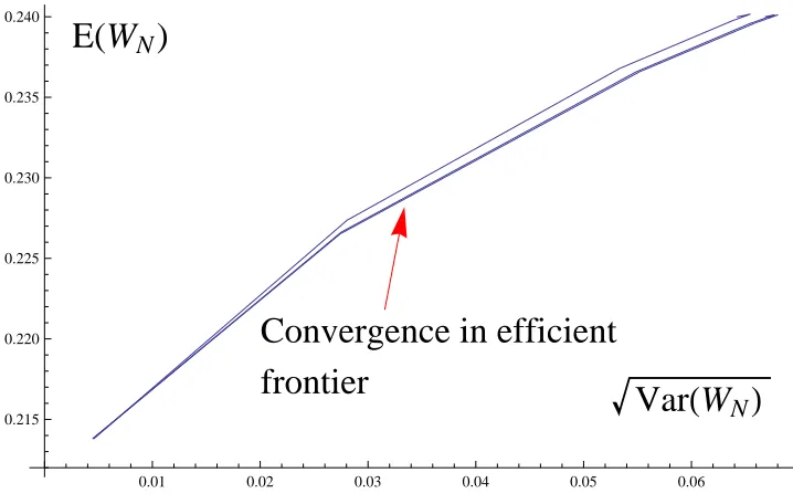
6.25 Impact of transaction cost on dynamic efficiency frontier with parametersT =

0.3,N = 6,s = e0.05∆T,m1 = 0.08, σ1 = 0.42,m2 = 0.14, σ2 = 0.8, ρ = 0.05.

WhereT is the time horizon for investment, N is the number of re-balancing nodes.ωis the continuous time risk-free rate, (λ, µ) are transaction cost factors,

s is the risk free growth over the interval, mi is the drift for continuous time

GBM and σi is the volatility for the continuous time GBM. The continuous

time GBM implies a risky growth for the risky asset over the interval∆T. . . . 112

6.26 Sharpe ratio time series evaluated at t = 0, initial fraction in asset one =0.5, initial wealth =0.2, for different times with parameters λ = µ = 0.005,T =

1,N = 10,s = e0.05∆T,m1 = 0.08, σ1 = 0.42,m2 = 0.14, σ2 = 0.8, ρ = 0.05.

WhereT is the time horizon for investment, N is the number of re-balancing nodes.ωis the continuous time risk-free rate, (λ, µ) are transaction cost factors,

s is the risk free growth over the interval, mi is the drift for continuous time

GBM and σi is the volatility for the continuous time GBM. The continuous

time GBM implies a risky growth for the risky asset over the interval∆T. . . . 113

6.27 Sharpe ratio series with myopic investment in individual assets evaluated at t=0 for different times with parameters λ = µ = 0.005,T = 1,N = 10,s = e0.05∆T,m1 = 0.08, σ1 = 0.42,m2 = 0.14, σ2 = 0.8, ρ = 0.05. Where T is the

time horizon for investment, N is the number of re-balancing nodes. ω is the continuous time risk-free rate, (λ, µ) are transaction cost factors, s is the risk free growth over the interval,mi is the drift for continuous time GBM andσiis

the volatility for the continuous time GBM. The continuous time GBM implies a risky growth for the risky asset over the interval∆T. . . 114

6.28 Obtaining infinite horizon solution using boundary update numerical methods with parametersm = 0.14, σ = 0.3, λ = µ = 0.05, ω = 0.1,s = eω∆T_{. Where}

T is the time horizon for investment,Nis the number of re-balancing nodes. ω is the continuous time risk-free rate, (λ, µ) are transaction cost factors, sis the risk free growth over the interval,mis the drift for continuous time GBM and

σ is the volatility for the continuous time GBM. The continuous time GBM implies a risky growth for the risky asset over the interval∆T. . . 115

6.29 Obtaining finite horizon no-transaction boundaries with parametersT =1,N =

10,m=0.08, σ= 0.42, λ= µ= 0.01, ω=0.05,s=eω∆T. Here iteration corre-sponds to the iteration in dynamic programming. WhereT is the time horizon for investment,Nis the number of re-balancing nodes.ωis the continuous time risk-free rate, (λ, µ) are transaction cost factors, s is the risk free growth over the interval,mis the drift for continuous time GBM andσis the volatility for the continuous time GBM. The continuous time GBM implies a risky growth for the risky asset over the interval∆T. . . 116

7.1 Parameters switching over the investment horizon. The three regimes have different drift and volatility for GBM of the risky asset. . . 120

(21)

7.2 Value of re-balancing for log-utility with initial risky fraction=0.5 and wealth

=1 the parametersλ= µ= 0.05,s= e0.05∆T,amin=0.001,amax=0.999,da=

0.01,T = 1,m = 0.14, σ = 0.6. WhereT is the time horizon for investment,

is the drift for continuous time GBM andσis the volatility for the continuous time GBM. The continuous time GBM implies a risky growth for the risky as-set over the interval ∆T. (amin,amax) are the bounds for risky fraction state space. . . 122 7.3 Value of re-balancing for log-utility with initial risky fraction=0.5 and wealth

=1 the parametersλ= µ= 0.05,s= e0.05∆T,_amin=₀.₀₀₁,_amax=₀.₉₉₉,_da=

is the drift for continuous time GBM andσis the volatility for the continuous time GBM. The continuous time GBM implies a risky growth for the risky as-set over the interval ∆T. (amin,amax) are the bounds for risky fraction state space. . . 123 7.6 Value of re-balancing when objective function is decomposed over small time

horizons to yield controls which are then applied to long-term value function with parametersλ = µ = 0.05,s = e0.05∆T,amin = 0.001,amax= 0.999,da =

0.1,T =1,m= 0.14, σ=0.6. WhereT is the time horizon for investment,Nis the number of re-balancing nodes.ωis the continuous time risk-free rate, (λ, µ) are transaction cost factors, sis the risk free growth over the interval,mis the drift for continuous time GBM andσis the volatility for the continuous time GBM. The continuous time GBM implies a risky growth for the risky asset over the interval∆T. (amin,amax) are the bounds for risky fraction state space. 124

(22)

7.7 Value of re-balancing with parameters that switch over the horizon -investor has perfect foresight. Each regime is of length 5/3 years. Parameters for first

m=0.4, σ=0.8; for secondm= 0.3, σ=0.7; and for thirdm=0.14, σ=0.6. AlsoT = 5, λ = µ= 0.05,s = e0.05∆T,amin= 0.001,amax = 0.999. WhereT

is the time horizon for investment, N is the number of re-balancing nodes. ω is the continuous time risk-free rate, (λ, µ) are transaction cost factors, sis the risk free growth over the interval,mis the drift for continuous time GBM and

σ is the volatility for the continuous time GBM. The continuous time GBM implies a risky growth for the risky asset over the interval∆T. (amin,amax) are the bounds for risky fraction state space. . . 125

7.8 Value of re-balancing for CRRA utility with initial risky fraction=0.5 and wealth

=1 the parameters V = 0.5, λ = µ = 0.05,s = e0.05∆T,_amin = ₀.₀₀₁,_amax =

0.999,da = 0.01,T = 1,m = 0.14, σ = 1.0. WhereT is the time horizon for investment, N is the number of re-balancing nodes. ω is the continuous time risk-free rate, (λ, µ) are transaction cost factors, s is the risk free growth over the interval,mis the drift for continuous time GBM andσis the volatility for the continuous time GBM. The continuous time GBM implies a risky growth for the risky asset over the interval∆T. (amin,amax) are the bounds for risky fraction state space. . . 126

(23)

=1 the parameters V = 0.5, λ = µ = 0.05,s = e0.05∆T,amin = 0.001,amax =

0.999,a = 0.01,T = 5,m = 0.4, σ = 1.5. Where T is the time horizon for investment, N is the number of re-balancing nodes. ω is the continuous time risk-free rate, (λ, µ) are transaction cost factors, s is the risk free growth over the interval,mis the drift for continuous time GBM andσis the volatility for the continuous time GBM. The continuous time GBM implies a risky growth for the risky asset over the interval∆T. (amin,amax) are the bounds for risky fraction state space. . . 129

=1 the parameters V = 0.5, λ = µ = 0.05,s = e0.05∆T,amin = 0.001,amax =

=1 the parametersV = 0.5, λ= µ= 0.05,s = e0.05∆T,amin = 0.001,namax =

0.999,da = 0.01,T = 5,m = 0.4, σ = 2. Where T is the time horizon for investment, N is the number of re-balancing nodes. ω is the continuous time risk-free rate, (λ, µ) are transaction cost factors, s is the risk free growth over the interval,mis the drift for continuous time GBM andσis the volatility for the continuous time GBM. The continuous time GBM implies a risky growth for the risky asset over the interval∆T. (amin,amax) are the bounds for risky fraction state space. . . 130

7.14 Value of re-balancing with parameters that switch over the horizon -investor has perfect foresight. Each regime is of length 5/3 years. Parameters for first

m=0.4, σ=1.2; for secondm= 0.3, σ=1.1; and for thirdm=0.14, σ=1.0. AlsoV = 0.5,T = 5, λ = µ = 0.05,s = e0.05∆T,amin = 0.001,amax = 0.999. WhereT is the time horizon for investment, N is the number of re-balancing nodes. ω is the continuous time risk-free rate, (λ, µ) are transaction cost fac-tors, s is the risk free growth over the interval, m is the drift for continuous time GBM andσis the volatility for the continuous time GBM. The continu-ous time GBM implies a risky growth for the risky asset over the interval∆T.

(amin,amax) are the bounds for risky fraction state space. . . 131

(24)

7.15 Scaled value of re-balancing for CARA utility with initial wealth in risky as-set =100 the parameters λ = µ = 0.05,s = e0.05∆T,amin = 0.001,amax =

7.16 Scaled value of re-balancing for CARA utility with initial wealth in risky as-set =100 the parameters λ = µ = 0.05,s = e0.05∆T,amin = 0.001,amax =

7.17 Value of re-balancing depicted by a shift in the efficiency frontier calculated for the initial wealth=0.2 and initial risky fraction=0.5. Parameters are chosen as:

T = 0.3, λ = µ = 0.005,s = e0.05∆T,_m

1 = 0.08, σ1 = 0.42,m2 = 0.14, σ2 =

0.8, ρ=0.05,amin=0.001,amax=0.999. . . 133

7.18 Mean variance CASE for AMAZON stock by forming a portfolio with risk free asset and AMAZON stock with parametersλ= µ= 0.01,s = e0.05∆T,T =

0.5,m = 0.18, σ = 0.4, λ = µ = 0.01. Where T is the time horizon for in-vestment, N is the number of re-balancing nodes. ω is the continuous time risk-free rate, (λ, µ) are transaction cost factors, s is the risk free growth over the interval,mis the drift for continuous time GBM andσis the volatility for the continuous time GBM. The continuous time GBM implies a risky growth for the risky asset over the interval∆T. . . 133

7.19 Log utility CASE for AMAZON stock by forming a portfolio with risk free as-set and AMAZON stock with parametersλ= µ= 0.01,s=e0.05∆T,T =1,m=

0.18, σ= 0.4, λ= µ= 0.01. WhereT is the time horizon for investment,N is the number of re-balancing nodes.ωis the continuous time risk-free rate, (λ, µ) are transaction cost factors, sis the risk free growth over the interval,mis the drift for continuous time GBM andσis the volatility for the continuous time GBM. The continuous time GBM implies a risky growth for the risky asset over the interval∆T. . . 134

(25)

7.20 CRRA utility CASE for AMAZON stock by forming a portfolio with risk free asset and AMAZON stock with parameters λ = µ = 0.01,s = e0.05∆T,T =

1,m = 0.18, σ = 0.4, λ = µ = 0.01. Where T is the time horizon for in-vestment, N is the number of re-balancing nodes. ω is the continuous time risk-free rate, (λ, µ) are transaction cost factors, s is the risk free growth over the interval,mis the drift for continuous time GBM andσis the volatility for the continuous time GBM. The continuous time GBM implies a risky growth for the risky asset over the interval∆T. . . 135 7.21 CARA utility CASE for AMAZON stock by forming a portfolio with risk free

asset and AMAZON stock with parameters λ = µ = 0.01,s = e0.05∆T,T =

1,m = 0.18, σ = 0.4, λ = µ = 0.01,z = 0.01. Value function is scaled and evaluated with initial wealth in risky asset=100. WhereT is the time horizon for investment,Nis the number of re-balancing nodes.ωis the continuous time risk-free rate, (λ, µ) are transaction cost factors, s is the risk free growth over the interval,mis the drift for continuous time GBM andσis the volatility for the continuous time GBM. The continuous time GBM implies a risky growth for the risky asset over the interval∆T. . . 136 7.22 Log-utility CASE: Phase geometry of no-transaction region with respect to

Merton point and mean-reversion of risky fraction with parameters λ = µ =

0.05,s = e0.1∆T,T = 6,N =80,amin= 0.001,amax= 0.999,da = 0.001,m =

0.14, σ=0.3. . . 136 7.23 CRRA utility CASE: Phase geometry of no-transaction region with respect

to Merton point and mean-reversion of risky fraction with parameters V =

0.5, λ = µ = 0.005,s = e0.05∆T,_T = ₁,_N = ₁₀,_amin = ₀.₀₀₁,_amax =

0.999,da=0.001,m=0.08, σ= 0.42. . . 137 7.24 CARA-utility CASE: Phase geometry of no-transaction region with respect

to Merton line with parameters λ = µ = 0.01,s = e0.05∆T,_T = ₁,_N =

10,xmin = 5,xmax = 600,dx = 1, η = 0.01,m = 0.18, σ = 0.4,z = 0.01. Here [xmin,xmax] denotes the bounds for amount of wealth in risky asset state space. Using the same parameters as estimated for AMAZON stock in this chapter. . . 137 7.25 CARA utility CASE: Phase geometry of no-transaction region with respect to

time varying Merton line η = 0.01, λ = µ = 0.01,s = e0.05∆T,T = 1,N =

10,xmin = 5,xmax = 600,dx = 1,m = 0.18, σ = 0.4,z = 0.01. Here

[xmin,xmax] denotes the bounds for amount of wealth in risky asset state space 138

7.26 Mean-variance (pre-committed controls -also called ’benchmark’ objective ) CASE: Phase stencil of no-transaction topology with respect to mean-reversion of risky fraction. Parameters are chosen as: T = 0.3,N = 6, λ = µ = 0.05,s = e0.05∆T,m1 = 0.08, σ1 = 0.42,m2 = 0.14, σ2 = 0.8, ρ= 0.05,amin =

0.001,amax= 0.999. . . 138 7.27 Reflection of the ’risky fraction’ process about the no-transaction boundaries

and the value of re-balancing. . . 139

8.1 Joint evolution discrete probability approximation for (risky growth, change in volatility. ) . . . 143

(26)

8.2 Evolution of risky growth. . . 146

8.3 Evolution of change in volatility. . . 146

8.4 Dynamic programming on a grid and truncation on volatility axis to avoid ex-trapolation errors. . . 147

8.5 Transaction cost processes. . . 148

8.6 No-transaction topology at time t=0.45 and parametersm =0.14, θ = 0.1,Λ = 0.8, ξ = 0.02,T = 0.5, ρ = 0.1, σmin = 0.5, σmax = 1.1, λ = µ = 0.01 +

0.01σ, γ = 2,L = 10Nγ,s = e0.05∆T,N = 10,da = amax_L−amin,∆T = T_N,amin =

0.001,amax = 0.999. Volatility axis horizontal and risky fraction axis verti-cal. We haveθ, Λ, ξ andρas the parameters for the joint evolution tee. Also

da represents the risky fraction space discretization with [amin,amax] being the bounds. WhereT is the time horizon for investment, N is the number of re-balancing nodes. ωis the continuous time risk-free rate, (λ, µ) are transac-tion cost factors, sis the risk free growth over the interval, m is the drift for continuous time GBM and σ is the volatility for the continuous time GBM. The continuous time GBM implies a risky growth for the risky asset over the interval∆T. . . 149

8.7 No transaction geometry at time t=0.1 and parametersm = 0.14, θ = 0.1,Λ = 0.8, ξ = 0.02,T = 0.5, ρ = 0.1, σmin = 0.5, σmax = 1.1, λ = µ = 0.01 +

0.01σ, γ = 2,L = 10Nγ,s = e0.05∆T,_N = ₁₀,_da = amax−amin

L ,∆T = T

N,amin =

0.001,amax = 0.999. Volatility axis horizontal and risky fraction axis verti-cal. We haveθ, Λ, ξ andρas the parameters for the joint evolution tee. Also

da represents the risky fraction space discretization with [amin,amax] being the bounds. WhereT is the time horizon for investment, N is the number of re-balancing nodes. ωis the continuous time risk-free rate, (λ, µ) are transac-tion cost factors, sis the risk free growth over the interval, m is the drift for continuous time GBM and σ is the volatility for the continuous time GBM. The continuous time GBM implies a risky growth for the risky asset over the interval∆T. . . 150

9.1 CRRA utility and no-transaction region for portfolio insurance constraint prob-lem at time =0.75 yrs with parameters: γN = ₁₀1,T = 1,N = 4, λ = µ =

0.01,s = e0.1∆T,_m = ₀.₁₄, σ = ₀.₃,_K = ₀.₂,_V = ₀._{5. We denote} _K _{as the}

portfolio insurance level. WhereT is the time horizon for investment,N is the number of re-balancing nodes. ω is the continuous time risk-free rate, (λ, µ) are transaction cost factors, sis the risk free growth over the interval,mis the drift for continuous time GBM andσis the volatility for the continuous time GBM. The continuous time GBM implies a risky growth for the risky asset over the interval∆T. γ` is the deformation parameter. Also V is the risk aversion

co-efficient for CRRA utility. . . 156

(27)

9.2 CRRA utility and no-transaction region for portfolio insurance constraint prob-lem at time=0 yrs with parameters: γN = ₁₀1,T = 1,N = 4, λ = µ= 0.01,s =

e0.1∆T,_m = ₀.₁₄, σ = ₀.₃,_K = ₀.₂,_V = ₀._{5. We denote} _K _{as the portfolio}

insurance level. WhereT is the time horizon for investment, N is the number of re-balancing nodes. ω is the continuous time risk-free rate, (λ, µ) are trans-action cost factors,sis the risk free growth over the interval,mis the drift for continuous time GBM andσis the volatility for the continuous time GBM. The continuous time GBM implies a risky growth for the risky asset over the inter-val∆T. γ`is the deformation parameter. AlsoVis the risk aversion co-efficient

for CRRA utility. . . 157

9.3 Here ? =BUY , =DO-NOTHING and •= SELL for no-transaction region geometry with CRRA utility for draw-down constraint problem at time=0.75 yrs and wealth =0.07 with parameters: γN = ₁₀1,T = 1,N = 4, λ = µ =

0.01,s = e0.1∆T,_m = ₀.₁₄, σ = ₀.₃, α = ₀.₂₅,_V = ₀._{5. We denote} α _as

important number in the draw-down constraint. WhereT is the time horizon for investment,Nis the number of re-balancing nodes.ωis the continuous time risk-free rate, (λ, µ) are transaction cost factors, s is the risk free growth over the interval,mis the drift for continuous time GBM andσis the volatility for the continuous time GBM. The continuous time GBM implies a risky growth for the risky asset over the interval∆T. γ` is the deformation parameter. Also V is the risk aversion co-efficient for CRRA utility. . . 158

9.4 Here ? =BUY , =DO-NOTHING and • = SELL for no-transaction region geometry with CRRA utility for draw-down constraint problem at time=0 yrs and wealth=0.07 with parameters: γN = ₁₀1,T = 1,N = 4, λ = µ= 0.01,s =

e0.1∆T,m=0.14, σ=0.3, α=0.25,V = 0.5. We denoteαas important number in the draw-down constraint. WhereT is the time horizon for investment, N

is the number of re-balancing nodes. ω is the continuous time risk-free rate, (λ, µ) are transaction cost factors, sis the risk free growth over the interval,m

is the drift for continuous time GBM andσis the volatility for the continuous time GBM. The continuous time GBM implies a risky growth for the risky asset over the interval∆T. γ` is the deformation parameter. AlsoV is the risk

aversion co-efficient for CRRA utility. . . 159

9.5 Initial wealth=0.5 and initial risky fraction=0.5. CRRA utility and terminal wealth distribution for portfolio insurance constraint problem with parameters:

γN = ₁₅1,T = 1,N = 4, λ = µ = 0.01,s = e0.1∆T,m = 0.14, σ = 0.3,K =

0.2,V =0.5. AlsoV is the risk aversion co-efficient for CRRA utility. . . 160

10.1 Trading Rule with entry and exit signals. . . 162

10.2 Transition diagram for the stateSk ∈ {N,S,L}. . . 163

10.3 Value function at timet =0 for spread process calibrated to “LOW” and “HD” stock pair. At t = 0 investor is short the spread with Z₀ = 1.0. The time horizon for trading is 0.5 years with 10 observation points and data calibrated to history from May 2011 to May 2012. . . 165

(28)

10.4 Simulation of gross realized profit (not including transaction costs) with trading starting at (2007,3,1) and look back of 500 days. The time horizon for trading is 0.5 years with 10 observation points and data calibrated with historical look back. . . 165 10.5 Simulation of gross realized profit (not including transaction costs) with trading

starting at (2007,3,1) and look back of 100 days. The time horizon for trading is 0.5 years with 10 observation points and data calibrated with the historical look back. . . 166 10.6 Histogram of realized profits for trading starting points chosen equally spaced

in 2005-2011. Stock pair is (LOW,HD). Look back of 180 days and trading horizon of 180 days. . . 167 10.7 Approximate dependence expected return of the MS stock on the (MS,GS)

stock pair spread using the daily closing stock prices from July 2005 to July 2006. . . 169 10.8 Approximate dependence expected return of the GS stock on the (MS,GS)

spread using the daily closing stock prices from July 2005 to July 2006. . . 169 10.9 Pair trading signals - shorting when the spread falls below a barrier and longing

when the spread goes above. . . 169 10.10Dynamic pairs trading - pair trading quadrants with different controls

illus-trated. . . 171 10.11Optimal control law at timet = 0 and spread=0.25 under dynamic trading for

the following choice of parameter which are already defined earlier : λ= µ = 0.005,T = 0.2,N = 2,s = e0.05∆T,_a = ₀.₁₆,_b = ₀.₁, σ

1 = 0.1,c = 0.1,d =

0.9, σ2 = 0.2, ρ = 0.05. Also ^ 7−→ SS, • 7−→SL, ? 7−→ LS, + 7−→LL and

]7−→NN. . . 176 10.12Optimal control law at time t = 0 and spread=0.5 under dynamic trading for

the following choice of parameter which are already defined earlier: λ = µ = 0.005,T = 0.2,N = 2,s = e0.05∆T,_a = ₀.₁₆,_b = ₀.₁, σ

1 = 0.1,c = 0.1,d =

0.9, σ2 = 0.2, ρ = 0.05. Also ^ 7−→ SS, • 7−→SL, ? 7−→ LS, + 7−→LL and

]7−→NN. . . 177 10.13Probability distribution of terminal wealth. . . 178

11.1 No-transaction geometries for growth rate maximization when parameters change over the horizon and investor has perfect foresight. Parameters:m1= 0.14, σ1 =

0.6,m2 = 0.2, σ2 = 0.5,m3 = 0.15, σ3 = 0.45. Here (mi, σi) is the drift and

volatility for regimei. . . 180 11.2 First passage time distribution using lattice compared to exact result. SQID

scheme used to create 25 branches for Standard Brownian motion. Parameters:

a = 0.25,N = 90,T = 0.2,wmin = −1,wmax = +1,mmin = −1,mmax =

+1,dw=0.05,dm =0.05. Hereais the barrier, Nis the number of time steps,

T is the time period, (wmin,wmax) are the bounds for actual value of Standard Brownian motion, (mmin,mmax) are the bounds for attained maximum value of Standard Brownian motion,dwis the size of state step inWk-space anddm

is the size of state step inMk space. . . 181

(29)

11.3 First passage time distribution using lattice compared to exact result. Moment matching of first 19 moments for Standard Brownian motion. Parameters:

a = 0.25,N = 90,T = 0.2,wmin = −1,wmax = +1,mmin = −1,mmax =

+1,dw=0.05,dm =0.05. Hereais the barrier, Nis the number of time steps,

T is the time period, (wmin,wmax) are the bounds for actual value of Standard Brownian motion, (mmin,mmax) are the bounds for attained maximum value of Standard Brownian motion,dwis the size of state step inWk-space anddm

is the size of state step inMk space. . . 182

11.4 Lattice framework for spread evolution. . . 183 11.5 No-transaction region variation with time for exchange rate model under a

sim-ple jump diffusion model with growth rate maximization for exchange rate portfolio. In the discrete time re-balancing we have no-transaction strips at

t = 0,0.25,0.5,0.75. Parameter choice is : T = 1,N = 4, λ = µ = 0.01,r1 =

e0.05∆T,r2= e0.07∆T,m= 0.14, σ=0.6, θ= 0.1, δ=0.05. . . 185

11.6 Realization of wealth for an investor trying to maximize Sharpe ratio by invest-ing in SP500 and GS startinvest-ing (2010,1,1) for one year with initial wealth=0.5 and initial fraction in SP500=0.5. Also Lookback=40 days. Paramater choice

T =1,N =5, λ= 0.005,r=0.05 . . . 186

(30)

List of Tables

2.1 Summary of Notations Used. . . 18

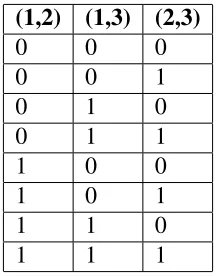
3.1 Transfer of wealth configurations between 3 risky assets where (i, j) is equal to 0 if he transfers fromito jand 1 if he transfers from jtoi. This table includes all the possibilities for transferring wealth under the control constraints. . . 28

3.2 A nice discrete probability approximation structure with correlated standard normals in 3-D . . . 42

5.1 Relative percentage error in value function with initial wealth=1, initial risky fraction=0.2, varying deformation from`=15 to 25 and parameter choice:λ=

µ= 0.01,s = e0.1∗∆T,_m = ₀.₁₄, σ = ₀.₃, γ

` = 1_`. WhereT is the time horizon

µ= 0.01,s = e0.1∗∆T,m = 0.14, σ = 0.3, γ` = 1_`. WhereT is the time horizon