by
Dimitrios I. Patsiatzis
A thesis su b m itte d for th e degree of D octor of Philosophy
of the University of London
July 2003
All rights reserved
INFORMATION TO ALL USERS
The quality of this reproduction is dependent upon the quality of the copy submitted.
In the unlikely event that the author did not send a complete manuscript and there are missing pages, these will be noted. Also, if material had to be removed,
a note will indicate the deletion.
uest.
ProQuest U642228
Published by ProQuest LLC(2015). Copyright of the Dissertation is held by the Author.
All rights reserved.
This work is protected against unauthorized copying under Title 17, United States Code. Microform Edition © ProQuest LLC.
ProQuest LLC
789 East Eisenhower Parkway P.O. Box 1346
savings at every stage of th e design process including th e process plant layout.
Decisions concerning th e plant layout may affect th e design, operation, production organisation, safety and construction of th e plant. This work aims at developing new q u an titativ e com puter-aided m ethods in order to assist engineers in generating
optim al process plant layouts to account for multifloor, safety and pipeless operation. A lot of research work from chemical and industrial engineers was m ainly focused on single-floor process plant layout following a variety of approaches w ithout con
sidering th e m ultifloor case in detail. M ultifloor constructions though can reduce significantly land and operational costs and comply w ith current requirem ents for m ore com pact plants. In this thesis efficient solution approaches are presented in
order to solve th e m ultifloor problem by determ ining th e num ber of floors and the spatial allocation of equipm ent item s to floors. A num ber of cost and m anage m ent / engineering drivers are considered w ithin th e sam e framework, thus resolving
various trade-offs at an optim al m anner. A wide range of plants, regarding the size and th e duty, have been tackled.
A num ber of accidents in chemical plants increased th e public awareness and antic
ipation for consideration of safety aspects during early stages of th e design process. So far, th ey have been included in a rath er simplified way in th e process plant layout problem and th e need for an in depth consideration is evident. Here, two different
T he pipeless batch plant problem has only recently a ttra c te d th e interest of the research com m unity. Layout decisions about th e allocation of processing stations
in th e land area are very im p o rtan t as th ey determ ine th e vessel transfer tim es
pervision, contribution and guidance. Financial support from th e C entre for Process
Systems Engineering and th e EPSRC is greatly acknowledged.
I am grateful to my best friend Tony for his support and hospitality and to my friends Donald, Lazaros, D im itris, Yiannis, Danny, Ahed, Keely, Monica, Alexis
and Billy.
M any thanks to all the past and present m em bers of th e UCL C A PE group and p articu larly to my friends Aris and N atalia.
1 In tr o d u c tio n 15
1.1 Aims and O b je c ti v e s ... 18
1.2 Thesis O u tlin e ... 19
2 L ite r a tu r e S u rv e y 21 2.1 Facility Layout and Location Problem ...22
2.2 Process P lant Layout P r o b le m ...24
2.3 Process Plant Layout with Safety A spects ... 28
2.4 Pipeless P lants ... 29
2.5 D is c u s s io n ... 31
3 M u ltiflo o r P r o c e s s P la n t L ayou t - A S im u lta n e o u s A p p ro a ch 34 3.1 The M ultifloor Process P lant Layout P r o b l e m ...35
3.2 M athem atical F o r m u la tio n ...36
3.2.1 Floor C o n s tr a in ts ... 38
3.2.2 Equipm ent O rientation C o n s t r a i n t s ... 40
3.2.3 Non-overlapping C o n s tr a in ts ...40
3.3 C om putational R e s u l t s ... 47
3.3.1 Instant Coffee P lant ... 48
3.3.2 Ethylene Oxide P l a n t ... 52
3.3.3 Batch P l a n t ... 54
3.3.4 C osm etic-grade Isopropyl Alcohol P l a n t ...56
3.4 Concluding R e m a r k s ... 57
4 M u ltiflo o r P r o c e s s P la n t L a y o u t - A D e c o m p o s itio n A p p ro a ch 63 4.1 A Decom position Solution A p p r o a c h ... 64
4.1.1 M aster P r o b le m ...65
4.1.2 Subproblem M o d e l ... 70
4.1.3 D ecom position Solution P r o c e d u r e ...72
4.2 C om putational R e s u l t s ...73
4.2.1 Instant Coffee P lan t ... 74
4.2.2 E thylene Oxide P l a n t ... 75
4.2.3 C osm etic-G rade Isopropyl Alcohol P l a n t ...77
4.2.4 Maleik A nhydride P l a n t ...78
4.3 Concluding R e m a r k s ...81
5.2.1 Instant Coffee P lant ... 90
5.2.2 E thylene Oxide Process ... 91
5.2.3 Cosm etic-G rade Isopropyl Alcohol P l a n t ... 92
5.2.4 Maleik Anhydride P l a n t ...94
5.2.5 C is-polybutadiene P l a n t ... 96
5.3 Concluding R e m a r k s ... 100
6 P r o c e s s P la n t L ayou t w ith S a fe ty A s p e c ts 107 6.1 An M INLP A p p ro a c h ... 108
6.1.1 Problem S t a t e m e n t ...108
6.1.2 M athem atical F o r m u la tio n ... 109
6.1.3 Illustrative Exam ple - Ethylene Oxide P l a n t ... 115
6.2 An MILP A p p ro a c h ... 117
6.2.1 The Dow Fire and Explosion Index S y s te m ... 119
6.2.2 Problem S ta te m e n t... 125
6.2.3 M athem atical F o r m u la tio n ...127
6.2.4 Illu strativ e Exam ple R e v is ite d ... 134
6.3 Concluding R e m a r k s ... 138
7 In te g r a tio n o f D e s ig n , L ayou t an d P r o d u c tio n P la n n in g for P ip e le s s
7.2.2 M aterial B a la n c e s ... 152
7.2.3 Station O ccupation C o n s t r a i n t s ... 152
7.2.4 Station O rientation C o n s t r a i n t s ...153
7.2.5 Non-overlapping C o n s tr a in ts ...154
7.2.6 Distance C o n s t r a i n t s ... 155
7.2.7 A dditional Layout Design C onstraints ...156
7.2.8 Vessels O ccupation C o n s t r a i n t s ... 157
7.2.9 O bjective F u n c t i o n ... 157
7.3 A Pipeless Batch P lant Exam ple ... 159
7.4 Concluding R e m a r k s ...164
8 C o n c lu sio n s and F u tu re D ir e c tio n s 167 8.1 Contributions of this th e s i s ... 167
8.1.1 Multifloor Process P lant L a y o u t... 167
8.1.2 Safe Process P lant L a y o u t ... 170
8.1.3 Sim ultaneous Layout, Design and O p e r a t i o n ... 171
8.2 Recom m endations for future Work ... 172
8.2.1 Iterative Solution A p p r o a c h ...172
8.2.2 CLP and H ybrid Approaches ... 173
3.1 Avoiding equipm ent overlapping (x- d ir e c tio n ) ...41
3.2 Avoiding equipm ent overlapping (y- d ir e c tio n ) ...42
3.3 Flowsheet for coffee plant ...48
3.4 O ptim al layout for coffee plant - Sim ultaneous approach ...50
3.5 Flowsheet for ethylene oxide plant ... 52
3.6 O ptim al layout for ethylene oxide plant - Sim ultaneous approach . . 54
3.7 Flowsheet for batch plant ... 56
3.8 O ptim al layout for batch plant - Sim ultaneous approach ... 58
3.9 Flowsheet for isopropyl alcohol p l a n t ... 60
4.1 Convergence for decom position approach for coffee p r o c e s s ...75
4.2 O ptim al layout for coffee process - Decomposition approach ... 76
4.3 O ptim al layout for ethylene oxide plant - Decom position approach . 76 4.4 Convergence for decom position approach for ethylene oxide plant . . 79
4.5 Convergence for decomposition approach for isopropyl alcohol plant . 79 4.6 O ptim al layout for isopropyl alcohol plant - D ecom position approach 80 4.7 Flowsheet for m aleik anhydride p l a n t ... 80
5.1 Convergence for iterative approach for coffee process ...91
5.2 O ptim al layout for coffee process - Iterative a p p r o a c h ... 92
5.3 O ptim al layout for ethylene oxide plant - Iterativ e a p p r o a c h ...93
5.4 Convergence for iterative approach for ethylene oxide process . . . . 93
5.5 Convergence for iterative approach for isopropyl alcohol plant . . . . 95
5.6 O ptim al layout for isopropyl alcohol plant - Iterative approach . . . 95
5.7 Convergence for maleik anhydride exam ple - Iterativ e approach . . . 97
5.8 O ptim al layout for m aleik anhydride exam ple - Iterativ e approach . . 97
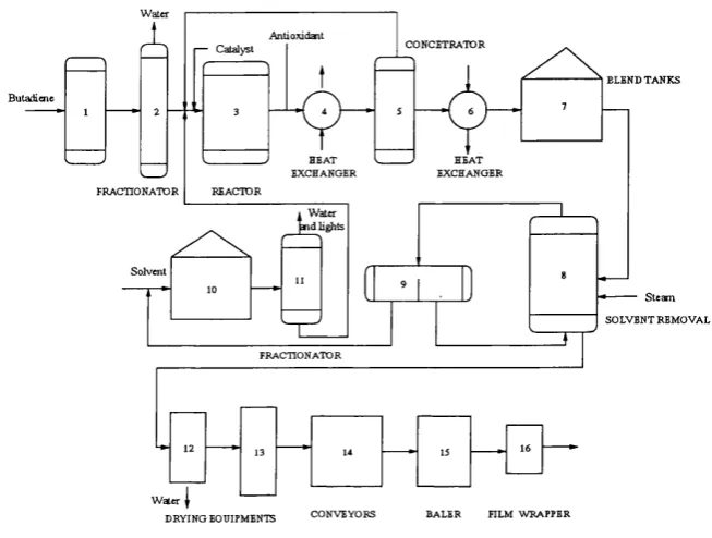
5.9 Flowsheet for cis-polybutadiene plant ... 98
5.10 O ptim al layout for cis-polybutadiene plant - Iterative approach . . . 99
5.11 Convergence for cis-polybutadiene plant - Iterative a p p r o a c h ...99
6.1 O ptim al l a y o u t ...118
6.2 O ptim al layout - No P rotection Devices ...118
6.3 Damage cost between source item i and ta rg e t item j ...130
6.4 O ptim al l a y o u t ... 137
6.5 O ptim al layout (Penteado and Ciric, 1996) 137 6.6 O ptim al layout - No protection Devices ... 140
7.1 Examples of pipeless plants l a y o u t s ... 143
7.2 Process state-task netw ork ... 144
7.3 O ptim al Layout ... 162
3.1 E quipm ent dimensions for coflFee plant ...49
3.2 C onnection and pum ping costs for coffee p l a n t ... 49
3.3 O ptim al solution for coffee plant - Sim ultaneous approach ... 51
3.4 E quipm ent dimensions for ethylene oxide p l a n t ... 52
3.5 C onnection and pum ping costs for ethylene oxide p l a n t ... 53
3.6 O ptim al solution for ethylene oxide plant - Sim ultaneous approach . . 55
3.7 E quipm ent dimensions for batch plant ...55
3.8 C onnection and pum ping costs for batch p l a n t ... 57
3.9 O ptim al solution for batch plant - Sim ultaneous approach ... 59
3.10 D imensions of equipm ent item s for isopropyl alcohol p lan t ... 60
3.11 C onnection and pum ping costs for isopropyl alcohol p l a n t ...61
3.12 O bjective function values in r m u ...62
3.13 Model sizes ...62
4.1 O ptim al solution for coffee process - Decom position a p p ro a c h ... 77 4.2 O ptim al solution for ethylene oxide plant - D ecom position approach . 78 4.3 O ptim al solution for isopropyl alcohol plant - Decom position approach 83
4.5 Connection and pum ping costs for m aleik anhydride p lan t ... 84
4.6 O bjective function values in r m u ... 85
4.7 CPU tim es in s ...85
5.1 O ptim al solution for colfee process - Iterativ e a p p r o a c h ... 94
5.2 O ptim al solution for ethylene oxide plant - Iterativ e approach . . . . 96
5.3 O ptim al solution for isopropyl alcohol plant - Iterativ e approach . . . lOI 5.4 O ptim al solution for maleik anhydride exam ple - Iterativ e approach . 102 5.5 Dimensions of equipm ent item s for cis-polybutadiene p l a n t ... 103
5.6 Connection and pum ping costs for cis-polybutadiene p l a n t ... 104
5.7 O ptim al solution for cis-polybutadiene plant - Iterativ e approach . . . 105
5.8 O bjective function values in r m u ...106
5.9 CPU tim es in s ... 106
6.1 Available protection d e v i c e s ...116
6.2 P rotection Device Costs ...117
6.3 P rotection Device R eduction F a c t o r ... 119
6.4 Param eters 0 h ... 120
6.5 Param eters 0 ^ 120 6.6 O ptim al Solution for Exam ple I ... 121
6.7 O ptim al solution for exam ple I- No Protection D e v i c e s ... 122
6.9 G eneral process hazards penalties ( F l i )...125
6.10 Special process hazards penalties ( F 2 i )... 126
6.11 Fire and explosion risk analysis system f a c t o r s ...126
6.12 E quipm ent dimensions and purchase c o s t ... 135
6.13 P rotection device d ata for th e r e a c t o r ...136
6.14 P ro tectio n device d a ta for th e ethylene oxide and carbon dioxide ab sorber ...138
6.15 O ptim al solution ... 139
6.16 O ptim al solution - No protection d e v i c e s ...140
7.1 P ro d u ct D a t a ...160
7.2 Processing Stations D a t a ... 161
7.3 O ptim al L o c a tio n ... 164
7.4 N um ber of b a t c h e s ... 165
7.5 O p tim al Location - Herringbone Layout ...166
In tr o d u c tio n
The process plant layout problem involves decisions concerning th e spatial allocation of equipm ent item s and th e required connections among them (M ecklenburgh, 1985). In general, th e process plant layout problem m ay be characterised by a num ber of cost a n d /o r m anagem ent/ engineering drivers such as:
• Connectivity C ost involving cost of piping and other required connections
between equipm ent item s. In addition, other related netw ork operating costs such as pum ping may be taken into account;
• Construction Cost: leading to th e design of com pact plants and particularly
significant in cases such as off-shore platform s. The trade-off between th e cost
of occupied area (land) and height (multi-floor plants) m ust also be considered;
• Retrofit: fitting new equipm ent item s w ithin an existing plant layout;
• Operation: involving scheduling issues (e.g. pipeless plants);
• Safety: introducing, for example, (constraints w ith respect to th e m inim um
allowable distance between specific equipm ent item s. Trade-offs between con nectivity, pum ping, construction, financial risk and installation of potential
protection devices will be considered; and
# Production Organisation: facilitatin g th e m ovements of goods and operators
through th e plant. Frequently, the accom m odation of a specific m anufacturing
p a tte rn (e.g. th e organisation of t h e workforce into team s, working in well
defined plant sections) m ay also be of great im portance.
Usually, plant layout decisions are ignored or do not receive appropriate atten tio n during th e design or retrofit of chem ical plants. However, increased com petition led contractors and chemical companies to look for potential savings at every stage
of th e design process by focusing th eir research on th e facility and process plant layout problem . Approaches for both problem s were based on heuristics, graph partitioning, stochastic optim isation and m ath em atical program m ing techniques as described in detail in chapter 2.
During th e layout of chem ical plants, th e re is a growing concern about safety aspects
th a t should be taken into account as th e y are usually not considered system atically
w ithin process layout, design and operation frameworks thus resulting in inefficient and unsafe plants. It is anticipated th a t safety aspects should be considered during early stages of th e design process by using appro p riate q u an titativ e indices. This
Pipeless batch plants have also recently received some atten tio n as alternative to
trad itio n al batch plants due to th eir inherent flexibility (m aterial can potentially be transferred between any two processing item s - stations). Layout considerations have been found to be of p articu lar significance in pipeless plants since th e location
of th e processing stations determ ines th e transfer tim es for th e moving vessels.
Some of th e m ost common lim itations of existing m ethodologies on th e above issues are th e following:
• Problem Representation: This should describe adequately the realistic charac
teristics of th e layout problem. The discrete-dom ain models, which have been used quite extensively, are often inadequate as th ey m ay provide suboptim al solutions or require significant com putational resources. In contrast, these deficiencies can be alleviated by continuous-dom ain models, which have only
recently a ttra c te d some atten tio n for academ ic interest. Most of these models
cap tu re only p a rt of the im p o rtan t layout issues, use unrealistic assum ptions (e.g. Euclidean distances) or are applied to single-floor plants;
• Multifloor Plant Layout: This is a more recent approach in order to capture
th e new requirem ents for m ore com pact plants and enclosed structures, the
use of gravity in m aterial transfer and the reduction of th e land area cost;
• Safety Aspects: These are either ignored or considered by sim plistic term s (e.g.
In addition, there is usually no account of financial risk and installation of potential protection devices; and
• Design and Operation: These should be considered sim ultaneously w ith plant
layout decisions in the case of pipeless plants where th ere are strong interac tions between th e above issues.
In this thesis, we focus on th e above lim itations by developing a system atic fram e work for th e optim al process plant layout.
1.1
A im s and O b je c tiv e s
This thesis aims at developing new qu an titativ e com puter-aided m ethods, which will assist process engineers in generating alternative chemical process plant layouts w ith reduced cost and enhanced safety.
The process plant layout problem can be defined as locating a given num ber of equipm ent item s in one or m ultiple floors so as to optim ise a perform ance criterion, subject to a variety of constraints determ ining orientation, non-overlapping, plant
area and distances between item s. Usually, th e perform ance criterion includes term s
such as piping cost, pum ping cost, land and construction costs, financial risk and cost of potential protection devices.
In order to achieve th e aim of delivering rigorous m ath em atical models and efficient solution m ethods for the plant layout problem , we set th e following key objectives:
• Multi-floor process plant layout;
• Safety; and
• Layout, design and operation.
2. The developm ent of optim isation-based algorithm ic m ethods for th e solution
of the resulting m ixed integer optim isation problem s.
In chapter 2, each of these points is considered in detail.
1.2
T h esis O u tlin e
The rest of th e thesis is stru ctu red as follows:
C hapter 2 presents a critical view of past work on single and m ulti-floor facility and process plant layout, safe process plant layout and sim ultaneous layout, design and operation of pipeless plants.
In chapter 3, a general m athem atical program m ing form ulation for th e multi-floor
process plant layout problem is presented. The m odel extends th e single-floor work of Papageorgiou and R otstein (1998), which is based on a continuous domain rep
resentation.
In chapter 4, a decom position approach capable of tackling larger flowsheets, w ithout
C h ap ter 5 presents a novel solution approach for th e m ulti-floor process plant layout problem based on an iterative solution scheme. T he new approach comprises of a
m aster and a subproblem as the decomposition approach, b u t a separate algorithm is followed for th e solution of the subproblem.
In chapter 6, two different m athem atical program m ing approaches - a m ixed-integer
nonlinear program m ing (M INLP) and a mixed integer linear program m ing (M ILP) model - considering th e process plant layout w ith safety aspects are presented. C h ap ter 7 suggests a unified m athem atical framework capturing layout, design, and planning aspects w ithin the sam e framework for pipeless plants.
L ite r a tu r e S u rv ey
P lant layout is concerned w ith spatial arrangem ent of equipm ent item s and can in fluence th e profitability of th e plant (M ecklenburgh, 1985). E quipm ent item s are allocated to one floor (single-floor case) or m any floors (multi-floor case) considering
a num ber of cost and m anagem ent/ engineering drivers {e.g. connectivity, opera tion, land area, safety, construction, retrofit, m aintenance, production organisation)
w ithin th e sam e framework. In order to resolve various trade-offs at an optim al
m anner, a num ber of com puter-aided m ethods have been developed.
The m ain research works in facility and process plan t layout problem s are reviewed in
sections 2.1 and 2.2 respectively. Works focused on th e safety aspects of th e process plant layout problem are presented in section 2.3. T he works related to pipeless
plants and th e ir layout issues are presented in section 2.4. Finally, in section 2.5 th e
m otivation and th e scope of this work is clarified in th e light of th e earlier work in this area.
2.1
F a cility L ayout and L o ca tio n P r o b le m
A first extensive approach of th e layout problem is given by industrial engineers
studying facility layout and location problem in Francis and W hite (1974), where a given num ber of departm ents are located in th e plane m inim ising th e m aterial
handling costs subject to location restrictions and dep artm en t and floor area re quirem ents. Comprehensive reviews on th e facility layout and location problem are
presented in Kusiak and Heragu (1987) and Meller and G au (1996).
T he most relevant approach for th e solution of th e single-floor facility layout prob lem is the Quadratic Assignment Problem (Q A P) (K oopm ans and Beckman, 1957). It is a special case of the facility layout problem as it assumes equal area d ep art m ents and a priori fixed and known locations. T he objective function depends on
th e flows (interactions) and th e distances between facilities. M any approaches are presented for th e solution of the QAP. Lawler (1963) suggests a transform ation of
th e Q A P into an equivalent integer linear program which is solved through a branch and bound technique. Fortenberry and Cox (1985) consider a heuristic approach
where the to tal work flow is first weighted according to closeness rating between departm ents and then minimised. Kaku et al. (1991) also present a com bination of
a constructive heuristic m ethod with exchange procedures. Combined m ethods to achieve q u an titative and qualitative goals are also suggested (B azaraa and Kirca,
1983; A dam s and Sherali, 1986). According to Kusiak and Heragu (1987) refor m ulations of th e QAP to include unequal area departm ents by breaking th em into
A nother approach for the solution of th e facility layout problem is based on graph
theory (Foulds, 1991) which maximises an objective function of weights of th e ad
jacencies (arcs) between departm ent pairs (nodes).
G enetic algorithm s also solve th e problem providing reasonably good layouts (Al-
H akim , 2000). T he flexibility of interactively modifying produced layouts or flxing departm ents is also considered (K ochhar et a l, 1998).
Finally, the single-floor facility layout problem is also solved in a continuous plane (avoiding th e requirem ent of knowing a priori the potential locations) using either mixed integer program m ing (M IP) models m inim ising a distance-based objective (M ontreuil, 1990) or MILP models, by applying a penalty m ethod to an uncon strained version of th e form ulation obtaining suboptim al solutions quickly (Heragu and K usiak, 1991).
A lim ited num ber of procedures are developed to solve th e m ulti-floor facility layout
problem . They can be divided in single stage and two-stage m ethods. In single stage procedures, departm ents are allowed to occupy any floor during execution.
Johnson (1982) presents an algorithm which is likely to split th em across different floors and is lim ited to exchange equal area or adjacent d epartm en ts between floors.
Bozer et al. (1994) overcome this lim itation by utilising space-filling curves. Both works employ search w ith the steepest-decent m ethod. M eller and Bozer (1996) on
In th e tw o-stage procedures though, each d ep artm en t is assigned perm anently to
each floor in th e first stage. In th e second stage th e layout is determ ined separately
for each floor. Kaku et al. (1988) solve th e first stage as a K -m edian problem (for equal area departm ents) and th e second stage as a QAP. Meller and Bozer (1997) present two procedures combining m ath em atical program m ing (first stage)
and sim ulated annealing (second stage). The second procedure perm it also th e reassignm ent of departm ents to different floors. A bdinnour-H elm and Hadley (2000) suggest two procedures where th e first stage is solved either as an MILP or following a greedy random ised adaptive search procedure (G R A SP) and th e second stage w ith ta b u search based heuristics. T he second stage procedure in all cases may give suboptim al solutions com pared to th e single stage one, b ut th e run tim es are considerably smaller.
2.2
P r o c e ss P la n t L ayout P r o b le m
Here, we focus on th e process plant layout problem where a given num ber of equip
m ent item s are located in th e plane m inim ising th e to ta l plant layout cost.
In th e single floor case, initial approaches are based on heuristic techniques which
th ey are efficient from th e com putational point of view bu t th ey do not guarantee o p tim ality of th e solution obtained. In Amorese et al. (1977), connection cost is
cost. E quipm ents item s are grouped into modules and th e m odules into sections
resulting in an M INLP model which is solved by a heuristic approach. Schm idt- Traub et at. (1998) develop a new m ethod for th e conceptual plan t layout problem
based on heuristic rules, statistical d ata and new algorithm s for th e new spatial
arrangem ent of equipm ent item s as well as pipe routing.
G raph th eo ry approaches are also applied to th e problem of organising item s into sections created by aisles or corridors by representing th e equipm ent and th eir con nectivities w ith an edge weighted graph (Jayakum ar and R eklaitis, 1994). Vertices are p artitio n ed into subsets and the to tal weight of th e edges joining vertices from different subsets is m inim ised.
F urtherm ore, stochastic optim isation techniques utilising genetic algorithm s are proved to be effective in obtaining good and practical solutions for th e enhanced
process p lan t layout problem w ith safety aspects (C astel et al., 1998).
A num ber of m ath em atical program m ing approaches are also suggested including
M INLP and MILP approaches. In Penteado and Ciric (1996), plant layout as pects are integrated w ith safety and economics. A disadvantage of this work is th e
adoption of circular footprints and straight-line connections (Euclidean distances)
between equipm ent item s. Both assum ptions are unrealistic as current industrial practices suggest rectangular shapes, in order to allow space for auxiliary in stru m en tatio n, piping and m aintenance, and rectilinear (M an h attan ) distances as the
R otstein, 1998).
Continuous dom ain M ILP models to determ ine optim al location [i.e. coordinates)
and o rientation for each equipm ent item are presented in Papageorgiou and R ot stein (1998). Two alternative form ulations are proposed accom m odating rectangu
lar equipm ent footprints. One of th e form ulations is then extended to account for
th e layout organisation into production sections.
An altern ativ e continuous form ulation for equipm ent allocation, utilising a piecewise-
linear function representation for absolute value functionals is presented in O zyruth and Realff (1999) where equipm ent orientation is not allowed. T he new form ula tion is com pared with th e one from Papageorgiou and R otstein (1998) and a hybrid form ulation is then suggested.
Finally, Barbosa-Povoa et al. (2001) propose an M ILP m odel considering different equipm ent orientation, distance restrictions, different connectivity inputs and o u t
p uts, irregular equipm ent shapes and space availability. T he m odel is then extended to address th e existence of production sections.
The m ultifloor process plant layout problem is a m ore recent approach in order to
capture:
• Cases where th e land area cost represents a considerable percentage of the to ta l cost due to th e geographical location of th e plant site and a possible
m ultifloor consideration may potentially reduce th e to ta l plant layout cost;
• Use of gravity in m aterial tran sfer to reduce operating costs considerably.
C urrent research works on this area include th e assignm ent of item s of m ultipurpose
batch plants to different floors, by taking into account vertical pum ping and land
costs and satisfying a num ber of preferences (Suzuki et ah, 1991b). A pproxim ations of th e tran sp o rtatio n and floor construction costs are used as th e exact distances are
not calculated. In Suzuki et ai (1991c), an integer program m ing m odel is proposed to arrange equipm ent item s of a batch plant in a m ulti-floor building. Various types of preferences are considered and each un it is divided or com bined w ith others into “com ponents” and each com ponent is assigned to one of th e “positions” on a grid. A com bination of a graphical heuristic approach and a m ath em atical program m ing form ulation in order to allocate th e units in different floors w ith no consideration of th e detailed layout w ithin each floor is proposed in Jay ak u m ar and Reklaitis (1996). T he heuristic approach provides an up p er bound and th e linearised integer nonlinear
program m ing (INLP) form ulation provides a lower bound to th e optim al solution.
A grid based M ILP m odel is described in Georgiadis et al. (1997), based on space discretisation into a set of candidate locations, w ith each equipm ent item occupying
only one location. T he objective function to be m inim ised was th e to tal pu m p ing, connection and floor construction cost. Georgiadis et al. (1999) adopt a finer
Finally, sim ilar to th e single floor approach, B arbosa-Povoa et al. (2002) present a num ber of topological characteristics in th ree M ILP m odels. T he first model de
scribes a basic 3D layout model while th e second and th e th ird one are extensions of
th e form er including multi-floor allocation of item s accounting for fixed and variable num ber of floors and height. Flowsheets up to 11 equipm ent item s are considered.
2.3
P r o c e ss P la n t L ayout w ith S a fe ty A s p e c ts
A ppropriate decisions on the process plant layout during th e design or retrofit of a chemical plant m ay increase the safety of th e plant. So far though, safety aspects are considered in a ra th e r simplified way by allocating equipm ent item s w ith respect to th e m inim um allowable distances between them . A num ber of accidents in chemical process industries in th e last two decades (K han and A bbasi, 1999) increased the
public awareness of hazards in industry, thus leading to a need for considering safety aspects in more detail w ithin process plant layout and design frameworks.
P articu lar attentio n to safety aspects of th e process plan t layout problem is given
through a heuristic approach by Fuchino et al. (1997), where th e equipm ent modules are divided into subgroups and then sub-arranged w ithin groups according to safety.
T hen, these sub-arrangem ents are merged.
G enetic algorithm m ethods utilising th e M ond Index (1995) also solve th e problem efficiently (Castel et a/., 1998). The M ond Index provides th e m inim um safety distances between th e process units and is chosen because of its sim plicity and
mining sim ultaneously th e process plant layout, th e num ber and ty p e of protection devices and th e financial risk associated w ith accidents and th eir propagation to
neighbouring item s, assum ing circular footprints of item s. This work is based in a
representation of th e risk related to accidents propagating from a source to a targ et item utilising th e equivalent T N T m ethod (Lees, 1980).
2.4
P ip e le s s P la n ts
New environm ental regulations, product specifications and dem ands and narrow profit m argins in the last 15 years have forced chemical industries to look for more effective ways of production operations to rem ain com petitive. A ttention is now focused on th e ad ap tab ility and flexibility of production operations of new plants or
revam ped existing plants. For exam ple, th e flexibility of batch plants on producing a large num ber of products is lim ited because of th e need of equipm ent and piping cleaning especially in food and pharm aceutical production.
One prom ising option is th e pipeless batch plants (Niwa, 1993). T heir m ain differ
ence from trad itio n al batch plants is the tran sp o rtatio n of m aterial through transfer
able vessels from one processing stage to th e other. T he vessels m ay have individual
built-in carts or m ay be carried by a shared pool of A u to m ated Guide Vehicles (AGVs) and their m otion can be free or take place on tracks. In th e later case
The processing takes place in processing stations of specific functions. According to Niwa (1991) th e following 6 processing station types are m ost oftenly included in
th e batch recipes: (a) mixing; (b) reaction; (c) distillation; (d) extraction/isolation;
(e) sam pling/discharge; and (f) washing station. T he sam e transfer vessels hold the m aterial while processing at each station. The elim ination of pipework offers great flexibility as any m aterial can be transferred in th e vessels between two different processing stations, offering quick respond to m arket dem ands. Cleaning performs
norm ally in cleaning stations reducing possible e x tra tim e of cleaning of th e stations and piping.
The pipeless plant problem have only recently a ttra c te d th e interest of th e research community. A heuristic m ethodology for th e design of single-stage pipeless plants is presented by Hasebe and H ashim oto (1991). A solution to th e aggregate problem of determ ining th e num ber of transferable vessels and processing stations and an
evaluation of th e pipeless plants considering operational issues is suggested in Niwa (1993) and Niwa (1994) respectively. Pantelides et al. (1995) present a system
atic and rigorous approach to th e optim al detailed short term scheduling of pipeless plants. The M ILP m odel exploits th e flexibility of th e plant equipm ents and ac
com m odates recipes of a rb itrary complexity. Liu and Me Greavy (1996) present
a fram ew ork which aims to consider and exam ine th e design and th e operating strategies of pipeless plants emphasising to dynam ic analysis and production ar
P lan t layout involves decisions about th e allocation of processing stations in th e
land area thus determ ining th e vessel tran sfer tim es and affecting th e scheduling
of b o th operation of processing stations and m ovem ent of vessels. Realff et ah
(1996) present a sim ultaneous approach considering design, layout and operation. A rigorous decom position procedure is proposed for th e solution of th e resulting MILP. T he layout stru ctu re is pre-selected and th e model decides th e position where each
statio n should be allocated (discrete approach). Gonzalez and Realff (1998a) couple a discrete event sim ulator to schedules derived from M ILP models and produce and com pare two different layouts w ith th e sam e equipm ent. Then th e sensitivity of th e M ILP schedules to random p ertu rb ation s in processing and travel tim es is evaluated.
Gonzalez and Realff (1998b) com pare th e above MILP schedules to results obtained by using local dispatch rules to govern station operation and vessel movement.
2.5
D isc u ssio n
In sections 2.1 and 2.2, th e m ain research works in th e facility and process plant
layout problem s were presented. Most applications of th e facility layout problem
consider job shops and assem bly facilities. Some of th e weaknesses of th e m ethods associated w ith th e facility layout problem are th e th e usual assum ptions of constant allocation of dep artm en ts to locations and equal area dep artm en ts and also th e
levels of com plexity of chemical processing.
T here are th re e basic disadvantages in th e approaches presented in section 2.2 for
th e process plant layout problem . T he first is th e provision of suboptim al solutions
as m any of th em are based on heuristic rules or consider discrete domain m od els. The second is th e non-com pliance w ith current in d u strial practices by utilising
Euclidean distances and circular footprints as clearly explained in th e works of Pen teado and Ciric (1996), Georgiadis et al. (1997) and Papageorgiou and R otstein (1998). Finally, m any of th em are unable to tackle large flowsheets in reasonable com putational tim es because of th e increased model size.
For these reasons, there is a need for new m ath em atical form ulations and new solu
tion approaches particularly in th e m ore prom ising and less investigated multifloor case to tackle large flowsheets in m odest com putational tim es utilising a continuous-
dom ain representation. In chapters 3, 4 and 5 a sim ultaneous, a decom position and an iterative approach are presented for th e solution of th e m ulti-floor process plant layout.
Considering safe process plant layouts, th ere is a need for an approach th a t combines
process p lan t layout and detailed risk assessment. In chapter 6, q u an titativ e safety evaluation system s like th e Dow Fire and Explosion H azard System (1994), which
quantifies th e expected dam age caused by fire or explosion, can be considered in a process p lan t layout problem .
such as financial risk and cost of protection devices. T he financial risk component
should reflect th e consequences of building unsafe chemical plants and can therefore be quantified as th e expected plant losses in case of accidents due to fire or explosion.
In chapter 6, a m ath em atical form ulation considering th e above issues by utilising
th e equivalent T N T m eth o d (Lees, 1980; A IC h E /C C P S , 1989) for th e representation of th e propagation of an accident from a source to a targ et unit.
Finally in th e case of pipeless plants, there is no approach deciding sim ultaneously on th e type of th e layout and the allocation of processing stations in th e land area of th e pipeless plant. T here is a need for a unified m ath em atical framework cap tu r ing layout, design, and planing aspects w ithin th e sam e fram ework. The resulting model should consider all th e above components sim ultaneously thus resolving var ious trade-offs at an optim al m anner. In C hapter 7 a new m ath em atical framework
is presented extending th e single-floor work of Papageorgiou and R otstein (1998), which is based on a continuous dom ain representation, and th e aggregate model
M u ltiflo o r P r o c e ss P la n t L ayou t
-A S im u lta n e o u s -A p p ro a ch
In this chapter, a sim ultaneous approach for th e m ultifloor process plant layout
problem is presented. T he proposed general m ath em atical program m ing form ula tion extends th e single-floor work of Papageorgiou and R otstein (1998), which is
based on a continuous dom ain representation. This type of representation com pares favourably to th e convenient, from th e m odelling point of view, grid-based approaches (Georgiadis et a/., 1997; 1999)) where equipm ent item s are allocated to
one or more candidate locations because they can guarantee global optim ality. The
M ILP form ulation determ ines sim ultaneously th e num ber of floors, land area, floor allocation of each equipm ent item and detailed layout for each floor.
In th e sim ultaneous approach presented here, rectangular shapes are assumed for
equipm ent item s following current industrial practices. R ectilinear distances be tween th e equipm ent item s are used for a more realistic estim ate of piping costs
(Penteado and Ciric, 1996; Papageorgiou and R otstein, 1998; Georgiadis et ah, 1999). Equipm ent item s, which are allowed to ro ta te 90°, are assum ed to be con
nected through their geom etrical centres.
Overall, th e multi-floor plant layout problem can be stated as follows:
Given:
• A set of N equipm ent item s and their dimensions;
• A set of K potential floors;
• C onnectivity network;
• Cost d ata (connection, pum ping, land and construction);
• Floor height;
• Space and equipm ent allocation lim itations; and
• M inim um safety distances between equipm ent item s.
Determine:
The num ber of floors, land area, equipment-floor allocation and detailed layout [i.e.
So as to m inim ise the to ta l plant layout cost.
N ext, th e m ath em atical form ulation is presented.
3.2
M a th e m a tic a l F o rm u la tio n
The indices and param eters associated w ith th e layout problem are listed below:
Indices
i , j equipm ent item
k floor
5 candidate rectangular area
Parameters
fij 1 if flow is from item i to item j ; 0 otherwise
ARs area of rectangular area s [m^]
C^j connection cost between item s i and j [rmu/m^]
C^j vertical pum ping cost between item s i and j [rmu/m]
C^j horizontal pum ping cost between item s i and j [rmu/m]
F C l fixed floor construction cost [rmu]
F C 2 area dependent floor construction cost [rm u/m ^]
L C land cost [rm u/m ^]
M distance upper bound
X s i Y s dimensions of rectangular area s [m]
ai^(3i dimensions of item i [m]
T he form ulation is based on th e following key variables:
Integer Variables
N F num ber of floors
Binary Variables
E l i j , E 2 i j non-overlapping binary variables (as used in Papageorgiou and Rotstein;
1998)
O i 1 if length of item i is equal to ai [i.e. parallel to x axis); 0 otherwise
Q s 1 if candidate area s is selected; 0 otherwise
Vik 1 if item i is assigned to floor k; 0 otherwise
Zij 1 if equipm ent item s i and j are allocated to th e sam e floor; 0 otherwise
Continuous Variables
U length of item i [m]
Xi^Ui coordinates of geom etrical centre of item i [m]
Aij relative distance in y coordinates between item s i and j , if% is above j [m]
Bij relative distance in y coordinates between item s i and j , if% is below j [m]
Dij relative distance in z coordinates between item s i and j , if z is lower th an j [m]
F A floor area [mS]
Lij relative distance in x coordinates between item s i and j , if z is to th e left of j
NQ^ linearisation variable expressing th e product of N F and Qs
Rij relative distance in x coordinates between item s z and i , if z is to th e right of
j [m]
TDij to ta l rectilinear distance between item s z and j [m]
Uij relative distance in z coordinates between item s z and j , if z is higher th a n j
[m]
ymax j^niensions of floor area [m]
3 .2 .1
F lo o r C o n s tr a in ts
Each equipm ent item should be assigned to one floor:
= 1 \/ ; (3.1)
Zij > Vi/c + Vjk — 1 Vz = 1..N — l , j = z + A: = 1..K (3.2)
Zij < 1 — K'/c + Vjk Vz = 1..N — = z + l . . N , k = 1..K (3.3)
Zij < 1 + — Vjk Vz = 1..7V — 1; j = i 1..N, k = 1..K (3.4)
Note th a t if two equipm ent item s z and j are allocated to th e sam e floor (z.e. Vk = Vjk) then th e corresponding Zij variable is forced to one by constraints (3.2), while constraints (3.3) and (3.4) are inactive. On the other hand, if equipm ent item s z and
j are allocated to different floors then constraints (3.2) are inactive while constraints (3.3) and (3.4) are active and force th e Zij variable to zero.
The num ber of floors, N F , is determ ined by:
% (3.5)
k
It should be added th a t constraints (3.5) will be active for th e equipm ent items
assigned to th e top occupied floor given th a t th e N F variable is minim ised in the
3 .2 .2
E q u ip m en t O r ie n ta tio n C o n s tr a in ts
T he length and th e depth of equipm ent item i are determ ined by equipm ent orien
ta tio n decisions. The effect of equipm ent orientation is captured as follows:
h = Oil ’ Oi + • (1 — Oi) V i (3.6)
di — OLi -\- Si ~ U V 2 (3.7)
3 .2 .3
N o n -o v e r la p p in g C o n s tr a in ts
In order to avoid situations where two equipm ent item s i and j occupy the same physical location when allocated to th e same floor [i.e. Zij = 1), appropriate con strain ts should be included in th e model th a t prohibit overlapping of their equipm ent footprint projections, either in a: or y direction. If i and j are allocated to th e same
floor, then this constraint is depicted in Figures 3.1 and 3.2. Non-overlapping is guaranteed if at least one of th e following inequalities is active:
Xi — Xj > ^ ^ ^ y i = 1..N — l , j = i \ . . N (3.8)
Xj — Xi > ^ \f i = 1..N — 1, j = i 1..N (3.9)
item j
I'igui'p 3.1: Avoiding e(;ni[)inent overlapping (x- direel ion)
dj + (Ij
Y ~ (3.11)
For instance, in Figure 3.1 inetpiality (3.9) is active while in Figure 3.2 inequality (3.10) is active. These non-overlapping disjunctive conditions can m athem atically he modelled by including appropriate “big M” constraints and introducing two ad
ditional sets of binary variables; Ei^j and E 2p. Each pair of values (0 or 1) to these variables determines which constraint from (3.8) to (3.11) is active.
For every pair (i, j ) such th a t j > i and Zp = 1, we have: If constraint (3.8) is active then :
item i
item j
Figure 3.2: Avoiding e(|ui])ment overlapping (y- direction)
constraint (3.9) is active then :
El,j =
i ,F2 -,j =
0If constraint (3.10) is active then :
El ,j = 0, E2,j = 1
If constraint (3.11) is active then :
EE j = ljE2ij = 1
In summary, the non-overlapping constraints included in the model are:
I-x j - X i + M - ( 2 - Z i j - E U j + E 2 i ^ ) > - C ^ • \ / i = l . . N - l , j = i + l . . N (3.13)
! / . - % + M .( 2 - Z.y + E l . j - E2.y) > 4 ^ Vz = = i + l..lV (3.14)
!/, - ÿ. + M - (3 - % - E l „ - E 2., ) > Vz = 1 . .7 V - l ,i = i + l..lV (3.15)
where M is an appropriate upper bound. Note th a t th e above constraints are inac tive for equipm ent item s allocated to different floors {i.e. Zij = 0).
3 .2 .4
D is t a n c e C o n s tr a in ts
T he single floor distance constraints presented in Papageorgiou and R otstein (1998)
are here extended for th e m ulti-floor case:
Rij — Lij = Xi — Xj V ( i , j ) : fij = 1 (3.16)
Aij - Bij = y, - yj \ / { i , j ) : fij = 1 (3.17)
Uij - Dij = H - ^ k • {Vik - Vjk) V (z ,i) : fij = 1 (3.18)
k
Thus, th e to ta l rectilinear distance between item s i and j is given by:
3 .2 .5
A d d itio n a l L a y o u t D e s ig n C o n s tr a in ts
Lower bound constraints on th e coordinates of th e geom etrical centre are included
in order to avoid intersection of item s w ith th e origin of axes:
x , > ‘j V i (3.20)
Vi > — V i (3.21)
A rectangular shape of land area is assumed to be used and its dimensions are
determ ined by:
X i + j < V i (3.22)
!/. + ! < VI (3.23)
These dim ensions are th en used to calculate the land area, FA:
F A = (3.24)
3 .2 .6
O b je c tiv e F u n c tio n
T he objective function of th e sim ultaneous model includes:
Vertical pum ping cost:
E E
Horizontal pum ping cost:
Floor construction cost:
F C l ■ N F + F C 2 N F - F A
• Land area cost:
Overall, th e problem is sum m arised as follows:
[Problem PO]
min
E E
[C‘,-TD „ + C:-Di, + Ctr(Jiii + Lii + Aij + Bii)]
F F C I ■ N F + F C 2 ■ N F ■ F A F L C - F A
subject to constraints (3.1) - (3.7) and (3.12) - (3.24).
The above problem is an M INLP model because of th e non-linearities involved in
th e last two term s of th e objective function and in equation (3.24). However, the
ji^max^ ymax variables required for the calculations of F A can be approxim ated sim
F A , will be chosen from a set of S candidate rectangular area sizes, ARs, w ith X s
and Ys dimensions. Then, binary variables, Qs, are introduced together w ith th e
constraints:
FA = Y , A R , - Q ,
(3.25)E < 3 » = 1 (3.26)
The values of and variables are forced to coincide w ith th e dimensions of the selected area size:
= (3.27)
= - Q , (3.28)
By introducing the above approxim ation, th e last two nonlinear term s of th e objec tive function now result in bilinear and linear term s, respectively. T he penultim ate
bilinear te rm can easily be linearised by introducing new continuous variables, NQ^:
fVQ, = . 0 , V 6
defined by:
= (3.30)
Finally, th e linearised problem corresponds to an MILP m odel which can be sum
m arised as follows: [Problem P]
+ F C 1 • N F + F C 2 NQ ^ F L C ■ F A
subject to
constraints (3.1) - (3.7), (3.12) - (3.23) and (3.25) - (3.30).
All continuous variables in th e form ulation are defined as non-negative.
N ext, a num ber of illustrative examples are presented to d em o n strate th e applica bility of th e MILP model [Problem P].
3.3
C o m p u ta tio n a l R e s u lts
In this section, th e proposed form ulation is applied to a num ber of previously pub
lished exam ples of process plant layout optim isation. All exam ples were modelled using th e GAMS modelling system (Brooke et ah, 1998) coupled w ith th e ILOG
Coffee
PERCOLATOR Hot water
SPRAY DRYER
Water CYCLONE
Dry instant coffee
PRESS
DRYER
Water
Wet coffee grounds
Figure 3.3: Flowsheet for coffee plant
candidate area sizes. It is also assum ed here th a t construction dimensions
and are available in m ultiples of 10 m. A floor height of 5m is selected for all
examples.
3 .3 .1
I n s ta n t C o ffee P la n t
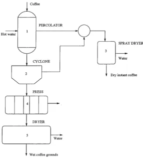
The first exam ple studied, is th e 5-unit instant coffee plant (see Figure 3.3), in tro
duced by Jay ak u m ar and R eklaitis (1996). Three potential floors are assum ed to be initially available.
are 3330 r m u and 66.7 respectively, and th e land cost param eter, LC, is
66.7 r m u / n F .
Table 3.1: Equipm ent dimensions for coffee plant
Unit 1 2 3 4 5
di [m] 1 5 ^ 1 2 15.8 6.3 9.5
A
[^] 3.2 3.2 3.2 6.3 3.2Table 3.2: Connection and pum ping costs for coffee plant
Connection C^j [ r m u /m] Oh [rmu/m] C-/j [rmu/m]
(1,2) 600 2525 25250
(1,3)
800 3783 37830(2,3) 350 631 6310
(2,4) 400 1879 18790
(4,5) 500 1420 14200
The resulting m athem atical model includes 211 constraints, 64 integer and 74 con
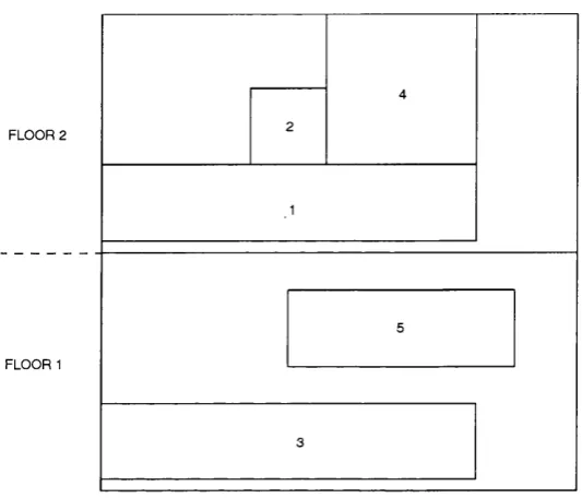
tinuous variables while th e optim al layout is shown in Figure 3.4. The optimal solution (equipm ent orientation and location, equipm ent-floor allocation) is gi\en
FLOOR 2
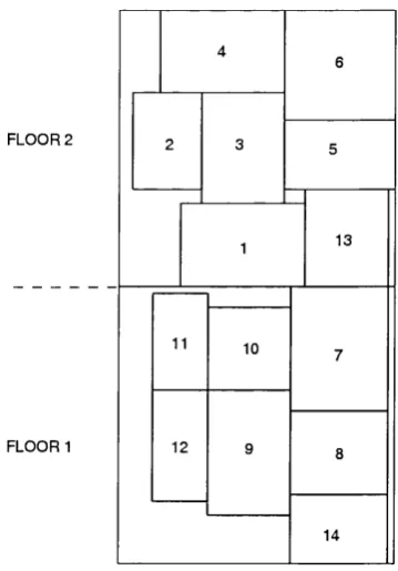
Figure 3.4: O ptim al layout for coffee plant - Sim ultaneous approach
from unit 2 to 3. It should be noted th a t two out of th e th ree initially available floors have finally been chosen. The to tal plant layout cost is 82366 r m u w ith the following breakdown: 16.8% for connection cost; 26.6% for horizontal and vertical pum ping costs, 16.17% for land and 40.43% for floor construction cost. The optim al
land area is 200 _ 2 0 rn, = 10 m ). T he corresponding CPU tim e is
3.1 5.
N ext, th e im portance of considering th e num ber of floors together w ith other layout
decisions {e.g. orientation, location) w ithin th e sam e optim isation framework is il lu strated . F irst, th e num ber of floors is assum ed to be fixed and th en th e reduced
M IL ? model is solved^. For th e single-floor case {i.e. NF=1), a suboptim al solu tion of 107497 r m u is obtained. This solution is 30.5% higher th an the two-floor
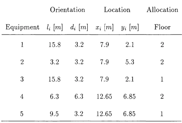
O rientation Location A llocation Equipm ent k [m] di [m] Xi [m] Vi [m] Floor
1 15.80 3.20 &50 7.90 2
2 T20 3.20 &50 4.70 2
3 1&80 T20 9.50 7.90 1
4 6.30 6.30 4.75 3.15 2
5 &50 3.20 4.75 3.15 1
optim al solution of 82366 rmu. Moreover, the three-floor optim al plant layout has an objective function of 89343 r m u which is also suboptim al (8.5% higher th an th e optim al value).
The cost breakdown for the single-floor case is: 10.3% for connection cost; 37.2% for
horizontal and vertical pum ping costs, 24.7% for land and 27.8% for floor construc tion cost. Com paring th e above breakdown w ith th e optim al one, it is obvious th a t
there is a significant increase in operating costs as gravity is not utilised any m ore
for m aterial transfer. Land cost is also increased as th ere is a need for a bigger land area to allocate all item s on th e same floor. On th e other hand, floor construction
■ o - ■ o
-HEAT
EXCHANGER EXCHANGERHEAT
Further processing
Purge
C02
ABSORBER
FLASH TANK
Vent
PUMP
Figure 3.5: Flowsheet for ethylene oxide plant
3 .3 .2
E th y le n e O x id e P la n t
Consider the ethylene oxide plan t, derived from th e case study presented by Pen- teado and Ciric (1996). The plan t flowsheet includes 7 units as shown in Figure 3.5. The equipm ent dimensions and the connection and pum ping cost d a ta are given in
Tables 3.4 and 3.5, respectively. T he F C l and F C 2 floor construction cost param e ters, are 3330 r m u and 6.7 rm u /m ^ , respectively, and th e land cost param eter, LC,
is 26.6 rmufm"^. T hree potential floors are assumed to be available.
Table 3.4: E quipm ent dimensions for ethylene oxide plan t
U nit 1 2 3 4 5 6 7
ai [m] 5.22 11.42 T68 8.48 7.68 2.60 2.40
Connection C^j [rmu/m] Cj/j [rmu/m] Cij [rmu/m]
(1,2) 200 400 4000
(2,3) 200 400 4000
(3,4) 200 300 3000
(4,5) 200 300 3000
(5,1) 200 100 1000
(5,6) 200 200 2000
(6,7) 200 150 1500
(7,5) 200 150 1500
The resulting m ath em atical model includes 382 constraints, 100 integer and 103 continuous variables and is solved in 174 s. The optim al layout is shown in Figure
3.6 com prising two floors. Equipm ent orientation and location and equipment-floor allocation are given in Table 3.6. The to tal plant layout cost is 50817 rm u w ith
the following breakdown: 23% for connection cost; 32.5% for horizontal and vertical
pum ping costs and 44.5% for land and construction costs. T he optim al land area is
400 = 20 m , = 20 m ).
As m entioned earlier, 25 (10m x 10m) candidate area sizes have been used for all examples. A finer discretisation of th e land area into 100 (5m x 5m) candidate areas will give a solution of 50137 r m u as th e land area is reduced to 375 m^. An
F L O O R 2
F L O O R 1
Figure 3.6: O ptim al layout for ethylene oxide plant - Sim ultaneous approach
optim al solution by 5.9% to 47797 rmu. From th e above values, it can be concluded
th a t there is a significant effect of the land area discretisation on th e to tal plant layout cost.
3 .3 .3
B a tc h P la n t
This exam ple was first proposed by Georgiadis et al. (1997). It considers th e layout
for an 11-unit batch plant (see Figure 3.7). The problem d a ta are presented in Tables
3.7 and 3.8. Floor construction cost param eters, F C l and 7^(72, are 3330 r m u and 3.33 respectively, and th e land cost param eter, L C , is 66.6 r m u f m ^ .
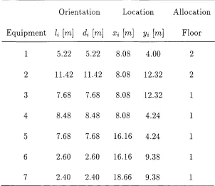
O rientation Location Allocation
E quipm ent h [m] di [m] Xi [m] Vi [m] Floor
1- 5.22 5.22 14.29 5T ^ 2
2 11.42 11.42 14.29 14.29 2
3 T68 7 ^ 8 14.29 14.29 1
4 8.48 8.48 14.29 6.21 1
5 T68 7 ^ 8 6.21 6.21 1
6 Z60 2 ^ 0 6.21 11.35 1
7 2.40 2.40 3.71 11.25 1
and construction cost 46.8 % of th e to ta l plant layout cost (37770 rmu). It should be noted th a t th ree out of five po ten tial floors have finally been chosen w ith an area of 100 _ 20 m , = 10 m) for each floor. T he size of th e model has
significantly increased from th e previous 7-unit exam ple as shown in Table 3.13.
Table 3.7: Equipm ent dimensions for batch plant
U nit V I V2 la lb 2a R2 R4 V5 V6 V5a V6a
ai [m] 5.0 6.0 4.0 6.5 6.0 4.0 4.0 5.0 4.0 2.0 3.0
V6a V5a R4
R 2
V5
V6
V2 V I
Figure 3.7: Flowsheet for batch plant
3 .3 .4
C o s m e tic -g r a d e Iso p r o p y l A lc o h o l P la n t
This exam ple was first presented in Jayakum ar and R eklaitis (1994) and considers th e layout design for a 12-unit plant (see Figure 3.9) m anufacturing cosmetic-grade
isopropyl alcohol. The equipm ent dimensions are given in Table 3.10. Connection and pum ping cost d a ta are given in Table 3.11. The floor construction cost param e
ters, F C l and FC72, are 2331 r m u and 9.9 r m u j m ^ , respectively, and th e land cost p aram eter, L(7, is 133.2 rmu/m"^. Four potential floors are initially available.
T he sim ultaneous approach appears incapable of solving this exam ple to optim ality.
Connection [rm u/m ] [rmu/m] C/j [rmu/m]
(V I,la ) 160 950 9500
(V 2,lb) 160 380 3800
(V2,R2) 160 570 5700
(la,2 a) 160 570 5700
(la,R 4 ) 160 190 1900
(lb ,2 a) 160 285 2850
(R2,R4) 160 456 4:560
(2a,V5) 160 456 4:560
(2a,V6) 160 304 3040
(R4,V5a) 160 285 2850
(R4,V6a) 160 285 2850
is capable of tackling flowsheets larger th an 11 units.
3.4
C o n c lu d in g R em ark s
In this chapter, a sim ultaneous approach for th e optim al m ulti-floor process plant layout problem has been considered. A general m ath em atical fram ew ork has been
FLOOR 3
FLOOR 2
FLOOR 1
V2
R4 R2
V1
1b
la
2a
Figure 3.8: O ptim al layout for batch plant - Sim ultaneous approach
so as to m inim ise th e to tal plant layout cost. The resulting optim isation problem corresponds to an MILP model. The applicability of th e proposed m odel has been
dem onstrated by four illustrative examples. As discussed earlier, th ere is a tra d e off between o p eratin g /lan d cost and floor construction cost which determ ines the
optim al num ber of floors and equipm ent layout.
Table 3.9: O ptim al solution for batch plant - Sim ultaneous approach
O rientation Location A llocation
E quipm ent h [m] di [m] Xi [m] Vi [m] Floor
V I 5 3 7.00 &00 3
V2 5 6 2 ^ 0 3.00 3
la 6 4 7.00 &00 2
Ib 5 6.5 7.50 3.25 3
2a 3 6 7.00 TOO 2
R2 5.5 4 2.75 3.00 2
R4 4 5 2.00 7.50 2
V5 3 5 7.00 3.00 I
V6 4 6 3.50 3.00 I
V5a I 2 0.50 7.50 I
V6a 2 3 2.00 7.50 I
Table 3.13. It is clear from th e above tables th a t th ere is a significant increase of
CPU tim e w ith th e exam ple size and the connectivity. In th e case of flowsheets with m ore th a n Il-u n its th e resulting model renders is difficult to solve. Therefore, th e need for th e developm ent of efficient solution procedures for th e multifloor process
Table 3.10; Dimensions of equipm ent item s for isopropyl alcohol plant
Unit 1 2 3 4 5 6 7 8 9 10 11 12
ai [m] 6.0 7.2 6.0 4.8 4.8 6.0 4.8 7.2 4.8 7.2 6.0 7.2
(3i [m] 4.8 6.0 7.2 6.0 6.0 4.8 6.0 4.8 6.0 6.0 4.8 4.8
Mixer ^ Reactor Scrubber Column Isopropyl-alcohol purification section Exchanger
WATER PROPYLENE
PRERUNNINGS
Storage
Desaller
INERTS 87.5 % 100%
ISOPROPYL ALCOHOL
Table 3.11: Connection and pum ping costs for isopropyl alcohol plant
Connection C^j [rmu/m] Ch [rmu/m] C^j [rmu/m]
(1,2) 120.0 939 9390
(2,3) 195.0 789 7890
(2.4) 135.0 909 9090
(3,2) 195.0 789 7890
(4.1) 12.0 42 420
(4,5) 45.0 210 2100
(4,6) 135.0 669 6690
(5,1) 42T 168 1680
(6,7) 135.0 669 6690
(7,8) 165.0 540 5400
(8,9) 90.0 570 5700
(8,11) 2T 0 72 720
(9,10) 90.0 420 4200
(10,11) 24.0 72 720
(11,7) 1T5 33 330
(11,12) 36.0 108 1080
(12,1) 12.0 42 420
![Figure 3.2: Avoiding e(|ui])ment overlapping (y- direction)](https://thumb-us.123doks.com/thumbv2/123dok_us/8308824.1378798/44.595.129.404.121.362/figure-avoiding-e-ui-ment-overlapping-y-direction.webp)