ECE-320 Lab 8: Utilizing a dsPIC30F6015 to control the speed of a wheel

1

ECE-320 Lab 8:

Utilizing a dsPIC30F6015 to control the speed of a wheel

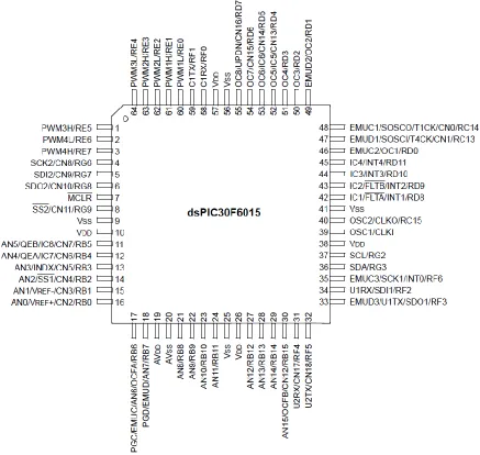
Overview: In this lab we will utilize the dsPIC30F6015 to implement P and PI controllers to control the speed of a wheel. Most of the initial code will be given to you (see the class website), and you will have to modify the code as you go on. One of the things you will discover is that you often need to be aware of limitations of both hardware and software when you try to implement a controller. The dsPIC30F6015 has been mounted on a carrier board that allows us to communicate with a terminal (your laptop) via a USB cable. In what follows you will need to make reference to the pin out of the dsPIC30F6015 (shown in Figure 1) and the corresponding pins on the carrier (shown in Figure 2)

2

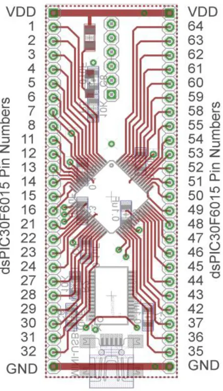
Figure 2. dsPIC30F6015 carrier. Note that the pin numbers are not consecutive.

Part A (Continuation of Lab7)

Start MPLAB X IDE (not IPE)

This lab is a continuation of Lab 7, so you will need to open the Lab7 project and continue to modify lab7.c

Part B: Reading in the sensor transducer (if necessary)

3 for the interface are shown in Figure 3. You need to connect this interface to +5 volts (red ), ground (blue), and the QEA Channel A input (pin 12), and the QEA Channel B input (pin 11).

Figure 3. Encoder pin outs.

Part C : Reading in an A/D value (if necessary)

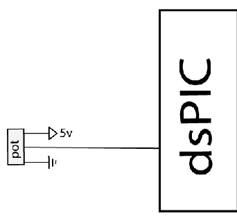
Now we want to be able to connect a potentiometer as shown in Figure 4 so we can have a variable reference. The software is currently set up for A/D input on AN3/RB3 (pin 13). You will need to do the following things:

 Connect the potentiometer as shown below

 Set the appropriate TRIS bits for an input signal

Note that this is the same set-up as was used in Lab7.

4

Part D: Connecting the power entry

Plug in both the 5 volt (green) and 12 volt (red) power supplies, as shown in Figure 5. Do not turn on the supplies yet (the LEDs should be off) .

Figure 5. Power entry module.

Part E: Connecting the H bridge

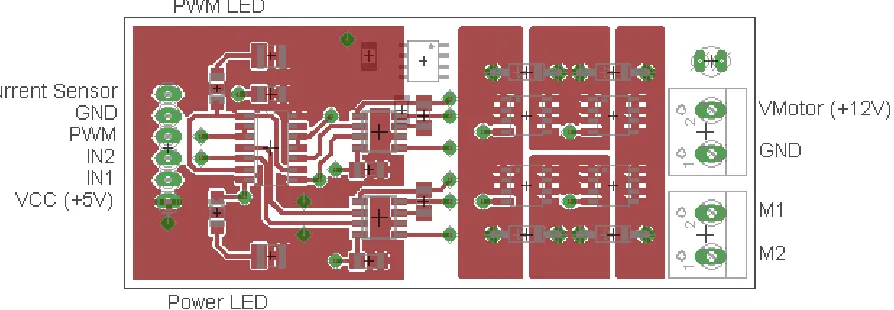
Plug in the H-bridge, shown in Figure 6. You are going to need access to the different pins, so be sure it is located in a place you can easily get wires to.

Figure 6. H Bridge connections

5 Starting on the right, connect (with the twisted wires) the 12 volt power from the power entry module to the 12 volt input. Be sure to connect ground to ground and +12 to +12. Next, connect M1 and M2 (using the twisted wires from the wheel) to the motor input.

At this point all of your wiring should be done. You should check it over before you go on.

Two important things to keep in mind as you do the remainder of this lab:

 Use the red switch to shut off power to the motor. Sometimes stopping the dsPIC does not stop the motor, in which case you will need to use the switch.

 Unless you are told otherwise (and later in the lab you will be), turn the pot fairly slowly.

For this lab, it is probably much easier to use the debugging features in MPLABX

Click here to compile and download to PIC

6

PART F: Plotting results

In the remainder of this lab you are to plot your results in Matlab. Once you have a good design, you need to log your data (File->Log Session in the SecureCRT window) so you can make a Matlab plot. If you have saved your data in a file named (for example) play3.log, then in Matlab type

data = load(‘play3.log’);

t = data(:,1);

y = data(:,5);

You may have to edit your files to make nice plots (like using t = t-t(1)). Be sure to include labels on your axes.

**************************** NEW STUFF **********************************

PART G: Proportional and derivative control

We need to include a derivative term to implement a full PID controller. You will need to define three new (double) variables, kd, Derror, and last_error. Outside of the main loop set last_error equal to zero and set kd equal to 0.01.

Inside the main loop include the lines

Derror = error-last-error; last_error = error;

Finally, to implement the full PID controller define the control error u to be

u = kp*error+ki*Isum+kd*Derror;

Click here to reset, this will stop the motor and

7 In designing a PD controller, you should set ki = 0. Start by adjusting the value of kp, and then add kd to speed up the system response. You will not likely get the correct steady state response, but do the best you can while meeting the settling time and percent overshoot requirements. We will add a prefilter in the next part to adjust the steady state value.

For each of the following steps, limit kp to less than 25 and kd greater than or equal to 0.1

a) With a set point of 45 rad/sec, adjust the gains kp and kd so the system reaches steady state within 0.5 seconds and with a percent overshoot less than 10%. Record the values of kp and kd and plot this result in Matlab and put it in your lab memo.

b) With a set point of 75 rad/sec, adjust the gain kp and kd so the system reaches steady state within 0.75 seconds and with a percent overshoot less than 10%. Record the value of kp and kd and plot this result in Matlab and put it in your lab memo.

c) With a set point of 90 rad/sec, adjust the gain kp and kd so the system reaches steady state within 0.75 seconds and with a percent overshoot less than 10%. Record the value of kp and kd and plot this result in Matlab and put it in your lab memo.

PART H: Proportional plus derivative control with a prefilter

Most likely your system did not equal the setpoint in steady state, or not all of them. Again we will use a prefilter to scale the input. The value of Gpf should be assigned once outside the main loop, and now needs to be determined. For previous step in the case where the reference input was 45, determine the ratio of the measured output to the setpoint, and use this as the initial value of Gpf. You may have to modify this value of Gpf, but once you choose one leave it fixed for the remainder of this part.

Now rerun the three cases from the previous part, and plot the results for each of them in Matlab. Include these plots in your memo. Note that you may not reach the correct steady state values (but you might). You should at least reach the correct steady state value of a reference of 45 rad/sec.

PART I: Designing a PID controller

At this point we want to design a general PID controller for each of the set points you have been using. Set the prefilter back to 1.0 for the remainder of this lab. Your steady state value should be within 2% of the setpoint within the specified settling time. A general plan for designing a PID controller using a trial and error method (we have no model for the plant) is the following:

 First, set ki = kd = 0, and try to get a good response for a step input using only kp.

 Next, adjust ki to get a good steady state error. Since the integral control tends to slow the system down, don’t make this any larger than you need to. However, you may need to also change

8 For each of the following steps, limit kp to less than 25, ki greater than or equal to 0.01, and kd greater than or equal to 0.01

a) With a set point of 45 rad/sec, adjust the gains so the system reaches steady state within 1.0 seconds and with a percent overshoot less than 10%. Record the values of kp, ki, and kd and plot this result in Matlab and put it in your lab memo.

b) With a set point of 75 rad/sec, adjust the gainso the system reaches steady state within 1.5 seconds and with a percent overshoot less than 10%. Record the value of kp, ki, and kd and plot this result in Matlab and put it in your lab memo.