Weak Deflection angle and Shadow by Tidal Charged Black Hole
Wajiha Javed,1,∗ Ali Hamza,1,† and Ali ¨Ovg ¨un2, 3,‡1Division of Science and Technology, University of Education,Township Campus, Lahore-54590, Pakistan 2Instituto de F´ısica, Pontificia Universidad Cat´olica de Valpara´ıso, Casilla 4950, Valpara´ıso, Chile.
3Physics Department, Arts and Sciences Faculty, Eastern Mediterranean University, Famagusta, North Cyprus via Mersin 10, Turkey. (Dated: March 2, 2020)
In this article, we calculate the deflection angle of tidal charged black hole (TCBH) in weak field limits. For doing this, first of all we obtain the Gaussian optical curvature and then apply the Gauss-Bonnet theorem on it and with the help of Gibbons-Werner method, we calculate the light’s deflection angle by TCBH. After calculating the deflection angle of light, we check the graphical behavior of TCBH. Moreover, we further find the light’s deflection angle in the presence of plasma medium and also check the graphical behavior in the presence of plasma medium. In the next section, we investi-gate the shadow of TCBH. For calculating the shadow, we first find the photon geodesic around the TCBH and then find its shadow. We also obtain TCBH’s shadow in the plasma medium. Moreover, we also find shadow’s shapes and discuss the effect of plasma on shadow.
PACS numbers: 95.30.Sf, 98.62.Sb, 97.60.Lf
Keywords: Relativity; Gravitation; Tidal Charged black hole; Gauss-Bonnet; Effect of Plasma; Shadow
I. INTRODUCTION
Einstein’s theory of general relativity (GR) is a wonderful gravity’s theory and was borned in 1916, Einstein in-telligently anticipated the presence of gravitational waves and gravitational lensing in his theory of (GR) [1]. Black Holes (BHs) are very interesting and captivating substance in the universe. It is assumed that various types of BHs are living in the universe but it is not confirmed experimentally till now. The black hole physics is very important because it plays a vital role in discovery of gravitational wave [2] and further BHs physics is used for more crucial level like entropy and the information paradox [3]. It also used in an interesting aspects of gravitational lensing. As indicated by Einstein, when light experiences an array of huge masses in its way towards the viewer then the light bends from the array and form the gravitational lens. When light passing from the array of galaxies then they divert the light’s path by using gravitational fields and in the background they generating disturbance for the origin. Strong lensing generates curves and rings, for example, the Einstein’s ring, while weak lensing is a consequence of small bends with amplifications too little to even think about detecting, except if found the middle value of over various systems.
The gravitational lensing is a useful system to comprehend the galaxies, dark matter of the universe, dark energy and the universe [4]. As the main gravitational lensing perception by the Eddington, a huge work on gravitational lensing have been accomplished for black holes, wormholes, cosmic strings and different items ([5]-[21]). Geodesic technique ([22]-[27]) was considered the main part for investigating the gravitational lensing and then in 2008, Gib-bons and Werner changed the circumstances by introducing the Gauss-Bonnet theorem (GBT) [28]. With the help of GBT, they find the light’s weak gravitational deflection in the static and spherically symmetric (SSS) spacetime e.g. Schwarzschild spacetime. In GBT the light’s deflection angle can be determined by integrating Gaussian curvature of related optical metric. In GBT we can utilize a spaceDR, which is limited by the photon beam just as a circular boundary curveCR which is situated at focus on the focal point here the photon beam meets the source and ob-server. It is expected that both origin and observer are at the coordinate distance R from the focal point. The GBT is communicated as pursues [28]:
Z Z
DR
KdS+
I
∂DR
κ dt+ Σiθi = 2πX(DR).
Here optical Gaussian curvature is denoted byKand an areal component is denoted by dS. Subsequently thinking about the Euler characteristic. X(DR) = 1, also added in the jump anglesΣiθi =π, the deflection angle is acquired
∗Electronic address:[email protected]; [email protected] †Electronic address:[email protected]
‡
Electronic address:[email protected]; URL:https://aovgun.weebly.com
by utilizing the adopting condition doing in consistence with the straight line estimate [28]:
α=−
Z π
0
Z ∞
b rsinφ
KdS.
Note that deflection angle is denoted byα. Then some other physicists study the light’s deflection angle using the GBT. For example, the deflection angle of light studied for BHs and wormholes by the following writers ([29]-[42]), Ovgun et al. studied for different spacetimes like Schwarzschild-like spacetime in bumblebee gravity model ([43 ]-[49]) and Javed et al. studied the impact of various matter fields ([50]-[54]). Next, Ishihara et al. [55] expressed that it is conceivable to calculate the finite-distances’s deflection angle (enormous effect parameter). As of late, Crisnejo and Gallo have contemplated the light’s deflection angle in the presence of plasma medium [56].
Most of the scientist said that a supermassive BH exist at the center of or galaxy and they hope that a far away viewer can see the supermassive BH as a dark space in the sky and it is called shadow of BH ([57]-[69]). Some say that which we called shadow, it is just the image of a event horizon and its size depend on the angle between the viewer and the event horizon according to Euclidean geometry. As a matter of fact, the shadow’s boundary compares to light beams that asymptotically access the photon circle and not the skyline. In addition, photon beams don’t move straight in Euclidean geometry yet they are bowed. Due to these reasons, the precise distance across of the shadow is really greater than the innocent Euclidean gauge recommends. For the dark gap at the focal point of our cosmic system, it adds up to around 53 `ıas though the Euclidean gauge gives just around 20 `ıas. At present, two ventures are in progress to watch the shadow that would give significant data on the minimal item at the focal point of our universe. These activities, which are going to utilize (sub)millimeter VLBI perceptions with radio telescopes appropriated over the Earth, are the Event Horizon Telescope and the Black Hole Cam [57].
The paper is organized as follows: in Section II we derive the optical metric and find the deflection angle in Section III. In Section IV we discus the graphical behavior and find the angle in the presence of plasma medium in Section V. Next, we find the graphical behavior in the presence of plasma in Section VI and calculate null geodesic in Section VII. Further we calculate shadow in Section VIII and also calculate shadow in the presence of plasma in Section IX and finally we conclude our results in Section X.
II. OPTICAL METRIC OF TCBH
The line element of a static, spherically symmetric TCBH is given by [70,71]
ds2=−B(r)dt2+ dr 2
B(r)+r 2dΩ2
2, , (1)
here
B(r) = 1− 2M
M2
pr
+ q
M2 5r2
,
and
dΩ22=dθ2+ sin2θdφ2,
here BH’s mass is denoted byMand the dimensionless tidal charge is denoted byqandMp(= 1.2∗1016T ev)denotes the effective Plank mass on the brane andM5denotes the fundamental Planck scale in the 5D bulk.
As both the origin and viewer lies in the same plane, so let(θ=π2). For obtaining optical metric we takeds2= 0,
dt2= dr 2
B2(r)+ r2dφ2
B(r). (2)
Now with the help of Eq.(2), the non-zero Christofell symbols are defined as
Γ000= B 0(r)
B(r) , Γ
1 01=
1 r−
B0(r) 2B(r)
and
Γ011=−rB+r 2B0(r)
and Ricci Scalar for optical metric is obtained as:
R=B00(r)B(r)−(B 0(r))2
2 . (3)
Then we calculate Gaussian optical metric as:
K=RicciScalar
2 .
After doing some simple calculation, Gaussian optical curvature is written as:
K ≈ −−2M
r3M2
p
− 6qM
r5M2
pM52
+ 3q
r4M2 5
+O M2, q2
. (4)
III. DEFLECTION ANGLE OF TCBH
In this section we find the deflection angle by TCBH with the help of GBT. We apply the GBT on this areaES, given as [28]
Z Z
FT
KdS+
I
∂FT
kdt+X
l
l= 2πZ(FT), (5)
hereKdenote the Gaussian curvature andkdenote the geodesic curvature as;k= ¯g(∇β˙β,˙ β¨)so,¯g( ˙β,β˙) = 1,β¨shows
unit acceleration vector and thelshows the exterior angle at the lth vertex. SinceT → ∞, both of the jump angles curtail toπ/2and then we haveθO+θT →π. Euler characteristic isZ(FT) = 1, asFT is non singular. So,
Z Z
FT
KdS+
I
∂FT
kdt+l= 2πZ(FT), (6)
here,l=πdemonstrates that bothα¯gand the total jump angle is a geodesic andZis the Euler characteristic number and it is equal to1. AsT → ∞, then we havek(ET) =| ∇E˙T
˙
EST|. Since, radial component of geodesic curvature is
written as [28]
(∇E˙T ˙
ET)r= ˙E φ
T∂φE˙Tr + Γ
0 11( ˙E
φ T)
2
. (7)
For largeT,ET :=r(φ) =T =const. Hence, the equation Eq.(7) becomes( ˙E φ T)
2= A2(r)B(r)
r2 . AsΓ 0
11=−rB+
r2B0(r)
2 ,
so it becomes
(∇E˙r T
˙
ETr)r→ −1
T . (8)
As geodesic curvature is free from topological defects so, k(ET) → T−1. By using the optical metric Eq.(4) and written asdt=T dφ. Hence, we have;
k(ET)dt=
1
TT dφ. (9)
By combining all the result we have,
Z Z
FT
Kds+
I
∂FT
kdt=T→∞
Z Z
U∞
KdS+
Z π+Θ
0
dφ. (10)
Light ray in week field limit at zeroth order is written asr(t) =b/sinφ. Using (5) and (11), the deflection angle is written as [28]
Θ =−
Z π
0
Z ∞
b/sinφ
Kpdet¯g drdφ, (11)
here√det¯g≈rdr.
After replacing the main terms of Gaussian curvature Eq.(4) into Eq.(11), the deflection angle is obtained as:
Θ ≈ 4M
bM2
p
− 3qπ 4b2M2
5
IV. GRAPHICAL ANALYSIS FOR NON-PLASMA MEDIUM
In this section we obtained the graphical behavior of TCBH’s deflection angle. We checked the graphical behavior in correspondence of deflection angleΘwith impact parameterbby varying the value of dimensionless tidal charge q. In these graphs we takeMpandM5are equal to 1.
A. Deflection angleΘw.r.t Impact parameterb
q=0.5
q=1
q=1.25
q=1.5
q=1.75
5 10 15 20
0.0 0.5 1.0 1.5
q
Θ
q=50
q=60
q=70
q=80
q=90
5 10 15 20
-70
-60
-50
-40
-30
-20
-10
q
Θ
Figure 1: Relation betweenΘandb.
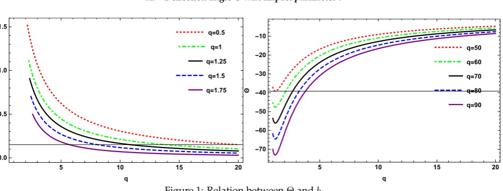
• Figure 1demonstrates the relation ofΘw.r.tbfor different values ofq.
1. In left plot, by considering the value of q = 0.5, deflection angle going to increase gradually and by increasing the values ofq’s the deflection angle decreases manually from graph ofq= 0.5and then going to increase toward positive side.
2. In right figure, graphical behavior shows the negative behavior and buy increasing the values ofq, deflec-tion angle also decrease toward negative side.
V. EFFECT OF PLASMA ON GRAVITATIONAL LENSING
In this portion we check that how a plasma medium effect the gravitational lensing of TCBH. Now, we assume the TCBH in the presence of plasma illustrated by the refractive indexn,[56]
n2(r, ω(r)) = 1− ω 2
e(r)
ω2 ∞(r)
. (13)
Here, refractive index is defined as in this case;
n(r) =
s
1− ω
2
e
ω2 ∞
1− 2M
M2
pr
+ q
M2 5r2
. (14)
and the line element is written as
ds2=−B(r)dt2+ 1 B(r)dr
2
+r2dΩ22 (15)
and
B(r) = 1− 2M
M2
pr
+ q
M2 5r2
.
as both the origin and viewer are in the same plane. So, put(θ= π2). For getting optical metric we letds2=0, as[56]
dt2=goptlmdxldxm=n2
dr2 B2(r)+
r2dφ2 B(r)
with determinantglmopt,
p
gopt=r(1− ω
2
e
ω2 ∞
) + M
M2
p(r)
(3 + ω 2
e
ω2 ∞
)− q
2M2 5r
(3 + ω 2
e
ω2 ∞
). (17)
By using Eq.(16),we can calculate the non-zero Christofell symbols as;
Γ000= (1 +ω 2 eB ω2 ∞ )
−B0B−1(1−ω 2
eB
ω2 ∞
)−B 0ω2
e
2ω2 ∞
,
Γ110= (1 +ω 2 eB ω2 ∞ )
r−1(1−ω 2
eB
ω2 ∞
−B 0B−1
2 (1−
ω2
eB
ω2 ∞
)−B 0ω2
e
2ω2 ∞
and
Γ011= (1 +Bω 2 e ω2 ∞ )
−rB(1−Bω 2
e
ω2 ∞
) +r 2B0
2 (1−
Bω2
e
ω2 ∞
) +r 2B
2 B0ω2
e
ω2 ∞
.
In terms of curvature tensor, the Gaussian curvature can be calculated in this way
K = −3 M ωe 2
r3ω ∞2Mp2
−2 M
Mp2r3
+ 5 qωe
2
ω∞2M52r4
+ 3 q
M2 5r4
−26 qM ωe 2
ω∞2M52Mp2r5
−6 qM
M2 5Mp2r5
(18)
With the help of GBT we obtained the deflection angle of TCBH in the presence of plasma medium and we relate it with non-plasma. So, for obtaining deflection angle in weak field limit, we apply the condition ofr = sinφb at 0th order.
Θ =−lim
R→0 Z π 0 Z R b sinφ
KdS, (19)
using this Eq.(10), the deflection angle of light in the presence of plasma medium is written as;
Θ = −6 M ωe
2
bω∞2Mp2
−4 M
bMp2 + 5/4
qωe2π
b2ω ∞2M52
+ 3/4 qπ b2M 52
+O(M2, q2, ω 3
e
ω3 ∞
). (20)
VI. GRAPHICAL ANALYSIS FOR PLASMA MEDIUM
In this portion we check that how TCBH’s deflection angle behave in the presence of plasma medium. Here, we take ωe
ω∞=10
−1and observe the deflection angle by changing the value of dimensionless tidal chargeq. We also take MpandM5are equal to 1.
A. Deflection angle w.r.t Impact parameter
q=0.5
q=1
q=1.25
q=1.5
q=1.75
5 10 15 20
-1.5 -1.0 -0.5 0.0 0.5 q Θ
q=50
q=60
q=70
q=80
q=90
5 10 15 20
-150 -100 -50 0 q Θ
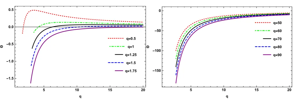
• Figure 2demonstrates the relation ofΘwithbfor different values ofb.
1. In 1st plot we observed that for value ofq = 0.5, the deflection angle first increase towards positive and then suddenly decrease toward negative side at some point. For values ofqgrater than 0.5, the deflection angle gradually decrease from positive to negative side and goes on toward the negative side.
2. In 2nd plot we observed that for large values ofqthe deflection angle goes towards the negative side and by increasing the values ofq, it continuously move toward negative side.
VII. NULL GEODESIC IN A TCBH
The Lagrangian representing the motion of light in the TCBH’s spacetime using this Eq.(1) is written as;
2L=−
1− 2M
M2
pr
+ q
M2 5r2
˙ t2+
1− 2M
M2
pr
+ q
M2 5r2
˙
r2+r2θ˙2+r2sin2θφ˙2, (21)
here derivative w.r.t affine parameterλis represented by an overdot. As Lagrangian is not depend on t andφso we introduce two new constants named as energyEand the angular momentumL. Where the values of these constants is defined as;
pt=
∂L
∂t˙ =−(1− 2M M2
pr
+ q
M2 5r2
) ˙t=−E (22)
and
pφ =
∂L
∂φ˙ =r
2sin2θφ˙=L.
(23)
For finding the restrictions of geodesic, we use these new introduced constants as;
dt dλ = ˙t=
E
1− 2M M2
pr+
q M2 5r2
, dφ dλ = ˙φ=
L
r2sin2θ.
Now, we define the new parts of momentum named asr-part andθ-par;
pr=
∂L ∂r˙ =
˙ r
1− 2M M2
pr+
q M2
5r2
and pθ=
∂L
∂θ˙ =r 2θ.˙
With the help of Hamilton-Jacobi equation, we find the values ofr-part andθ-part of the geodesic equation as;
∂S ∂λ =−
1 2g
µν ∂S
∂xµ
∂S
∂xν, (24)
and for photons(m0= 0), Eq. (24) can give us result of the following type,
S=−Et+Lφ+Sr(r) +Sθ(θ), (25)
whereSrdepends onrandSθ depends onθ. Now we get the Carter constant(±K)[66] by separating the values ofrandθand we get these values ofrandθby replacing Eq. (25) into Eq. (24) and also substituting the values of contravariant metric, i.e.,gµν, we have
1
q
1− 2M M2
pr+
q M2 5r2
dr dλ =
+ −
√
R(r),
r2dθ dλ =
+ −
√
T(θ), (26)
here the values ofRandθcan be defined as,
R(r) = E
2
1− 2M M2
pr+
q M2 5r2
− K
r2,
T(θ) =K − L 2
Now, EquationSrcan be written as
dr dλ 2
+Vef f = 0, (28)
with
Vef f =−
1− 2M
M2
pr
+ q
M2 5r2
R(r). (29)
We see that effective potential depend on BH’s mass denoted byM and the dimensionless tidal charge denoted by qand effective Plank mass on the brane denoted byMp and fundamental Planck scale in the 5D bulk denoted by
M5and radiusrandR(r). Now we change these parameters to new impact parameters such asξ= LE andη =EK2.
Now we change the value ofRwith respect to these new impact parameters.
R=E2[ 1
1− 2M M2
pr+
q M2 5r2
− η
r2]. (30)
VIII. SHADOW OF TCBH
Here, in this section we find the shadow of TCBH and we discussed in detail about shadow in the introduction. Now for finding the shadow, we find the unstable circular photons orbits. For this we must satisfy this,
R= 0 and R0 = 0, (31)
where prime(0)means differentiation w.r.tr. Putting (30) into (31), we obtained
η+ξ2= r 2
B(r) (32)
and
B0(r) B(r) =
2
r. (33)
the photon sphere radiusris found as follows:
η= r
2
1− 2M M2
pr+
q M2 5r2
, r= 3M
2M2
p
+
q9M2
M2 p −
8q M2
5
2 . (34)
Where impact parameters depends on BH’s mass denoted byM and the dimensionless tidal charge denoted byq and effective Plank mass on the brane denoted byMpand fundamental Planck scale in the 5D bulk denoted byM5
and radiusr. So Eq. (34) give detail about the boundary of the shadow and an observer which is far away from the BH can find this shadow in this sky and we make new coordinates in the observer’s sky named as the celestial coordinates (α,β), and we relate these coordinates with impact parameters (ξ,η). These coordinates are defines in these papers ([67],[68]) as;
α=limr0→∞(r20sinθ0)dφ dr,
β=limr0→∞ r20 dθ
dr, (35)
Wherer0 represents the distance between the viewer and the BH andθ0 denotes the angular coordinates of the
observer called ”inclination angle”. After putting the equations of four-velocities into Eq. (35), and doing some calculation, we obtain these celestial coordinates as,
α=− ξ
sinθ0
and β=
s
η− ξ
2
sinθ2 0
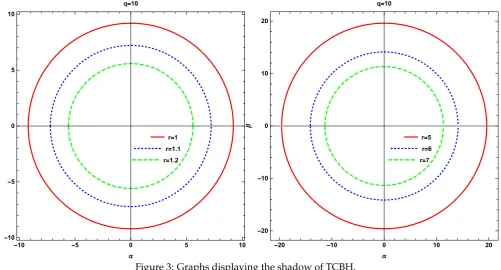
With the help of these equations and using the impact parameters we now make the shape of TCBH’s shadow and for plotting the shadows’s shape we plotαversusβwhich give detail about the boundary of the TCBH in the observer’s sky and these plots are seen in the Fig 3.
r=1 r=1.1 r=1.2
-10 -5 0 5 10
-10 -5 0 5 10
α
β
q=10
r=5
r=6
r=7
-20 -10 0 10 20
-20
-10
0 10 20
α
β
q=10
Figure 3: Graphs displaying the shadow of TCBH.
We plots the different graphs by changing the values of the dimensionless tidal chargeqand radial coordinater, in these plots we discuss about the shadow for small and large values ofq and by varying the values ofrin the equatorial plan by puttingθ0=π2. We saw that shadow’s shape is a perfect square and its shape as shown in Fig. 3.
In these graphs we see that for small values ofrand for large values ofrshadow shows the same behavior for fix vale ofq= 10and shadow is decreasing by increasing the value ofr.
IX. EFFECT OF PLASMA ON SHADOW OF TCBH
In Paper [69] we discuss in detail about the formula of the calculating the formula of shadow of a spherically symmetric spacetime. The line element of spherically symmetric TCBH is defined in this Eq.(1) and we can write as
ds2=−A(r)dt2+ dr 2
B(r)+r 2dΩ2
2, (37)
here
A(r) = [B(r)]−1= 1− 2M
M2
pr
+ q
M2 5r2
, and D(r) =r2,
and here we also check the TCBH’s shadow in the presence of plasma medium. The refractive indexncan be written as;
n2(r, ω(r)) = 1−ω 2
e(r)
ω2 ∞
. (38)
Here from reference[69], w can define theh(r)as;
h(r2) =r2 1 1− 2M
M2 pr+
q M2 5r2
−ω 2
e(r)
ω2 ∞
!
We can calculate the radius of a photon sphere by computing the above equation as,
0 = d
dr
h(r)2 (40)
In this case the value ofh(r)is defined by (39) and we use circumstances (40) for a photon sphere becomes
0 =
4r3(r2−2M r M2
p +
q M2
5 )−r4
r2−2M r M2
p +
q M2
5
2 −2r
ω2
e(r)
ω2 ∞
−2r2ωe(r)ωe(r 0)
ω2 ∞
. (41)
Angular radius of the shadow is defined as,
sin2αsh=
r2
ph
1 1− 2M
M2 p rph
+ q
M2 5r2ph
−ω2e(rph)
ω2 ∞ ! r2 ph 1 1− 2M
M2 p rph
+ q
M2 5r2ph
−ω2e(rph)
ω2 ∞
! (42)
whererphhas to be determined from (42). For vacuum,ωe(r) = 0, our consideration gives
h(r2) =r2 1 1− 2M
M2 pr+
q M2 5r2
!
. (43)
and
sin2αsh=
r2
ph
1 1− 2M
M2 p rph
+ q
M2 5rph2
!
r2
ph
1 1− 2M
M2 p rph
+ q
M2 5rph2
! (44)
where the positive value ofrphcan be calculated as;
rph=
1 + 2MM2 p+
q
(1 + 2MM2 p)
2− 4q M2
5
2 (45)
X. CONCLUSION
In this paper, we first of all find the deflection angle of TCBH with the help of Gaussian curvature. We find the angle by a famous theorem named as GBT proposed by Gibbons and Werner. The deflection angle is described as
Θ ≈ 4M
bM2
p
− 3qπ 4b2M2
5
+O(M2, q2). (46)
This shows that angle depends on BH’s mass denoted byM and the dimensionless tidal charge denoted byqand effective Plank mass on the brane denoted byMpand fundamental Planck scale in the 5D bulk denoted byM5and
impact parameterb. After calculating the deflection angle of TCBH we check its graphical behavior by varying the values ofqand by fixing all the other constants. In the next step we move toward the deflection angle of TCBH in the presence of plasma medium. We find this angle also by the same method named as GBT. This angle in the presence of plasma is defined below
Θ = −6 M ωe
2
bω∞2Mp2
−4 M
bMp2 + 5/4
qωe2π
b2ω ∞2M52
+ 3/4 qπ b2M 52
+O(M2, q2, ω 3
e
ω3 ∞
). (47)
After neglecting the plasma medium effect we find the same angle as we find in the non-plasma case. Now if we neglect the plasma effect(ωe
the correctness of our angle in the presence of plasma medium. After calculating the effect of plasma, we find the graphical behavior of TCBH in the presence of plasma medium. It does not shows the same behavior as the behavior without plasma.
Now in this paper we also find the shadow of TCBH, for this we first of all find the Null geodesic of TCBH and then convert it to new impact parameters named as energyEand the angular momentumL. After that we calculate the shadow and shows his image in the far away observer’s sky, for this we convert our results into celestial coordinates (α,β). After calculating the shadow, we plots the graphs of the shadow and discuss it by varying values of radial coordinate r. We also discuss the shadow of TCBH in the presence of plasma medium and discuss its effect on shadow of TCBH.
Acknowledgments
This work was supported by Comisi ´on Nacional de Ciencias y Tecnolog´ıa of Chile through FONDECYT GrantNo
3170035 (A. ¨O.).
[1] A. Einstein, Science 84, 506 (1936)
[2] B. P. Abbott et al. [LIGO Scientific and Virgo Collaborations], Phys. Rev. Lett. 116, no. 6, 061102 (2016). [3] S. D. Mathur, Class. Quant. Grav. 26, 224001 (2009).
[4] M. Bartelmann, Class. Quant. Grav. 27, 233001 (2010).
[5] C. R. Keeton, C. S. Kochanek and E. E. Falco, Astrophys. J. 509, 561 (1998). [6] A. Bhadra, Phys. Rev. D 67, 103009 (2003).
[7] R. Whisker, Phys. Rev. D 71, 064004 (2005).
[8] S. b. Chen and J. l. Jing, Phys. Rev. D 80, 024036 (2009).
[9] K. K. Nandi, Y. Z. Zhang and A. V. Zakharov, Phys. Rev. D 74, 024020 (2006). [10] E. F. Eiroa, G. E. Romero and D. F. Torres, Phys. Rev. D 66, 024010 (2002). [11] S. Mao and B. Paczynski, Astrophys. J. 374, L37 (1991).
[12] V. Bozza, Phys. Rev. D 66, 103001 (2002).
[13] H. Hoekstra, H. K. C. Yee and M. D. Gladders, Astrophys. J. 606, 67 (2004). [14] K. S. Virbhadra and G. F. R. Ellis, Phys. Rev. D 65, 103004 (2002).
[15] O. Gurtug and M. Mangut, Phys. Rev. D 99, no. 8, 084003 (2019) [16] K. S. Virbhadra and G. F. R. Ellis, Phys. Rev. D 62, 084003 (2000). [17] O. Kasikci and C. Deliduman, Phys. Rev. D 100, no. 2, 024019 (2019) [18] E. Gallo and O. M. Moreschi, Phys. Rev. D 83, 083007 (2011). [19] G. Crisnejo and E. Gallo, Phys. Rev. D 97, no. 8, 084010 (2018). [20] M. Sharif and S. Iftikhar, Astrophys. Space Sci. 357, no. 1, 85 (2015). [21] G. W. Gibbons, Phys. Lett. B 308, 237 (1993).
[22] S. Weinberg, Gravitation and Cosmology: Principles and Applications of the General Theory of Relativity (Wiley, New York, 1972).
[23] A. Edery and M. B. Paranjape, Phys. Rev. D 58, 024011 (1998). [24] J. Bodenner and C. Will, Am. J. Phys. 71, 770 (2003).
[25] K. Nakajima and H. Asada, Phys. Rev. D 85, 107501 (2012). [26] W. G. Cao and Y. Xie, Eur. Phys. J. C 78, 191 (2018).
[27] C. Y.Wang, Y. F. Shen and Y. Xie, J. Cosmol. Astropart. Phys. 04 (2019) 022. [28] G. W. Gibbons and M. C. Werner, Classical Quantum Gravity 25, 235009 (2008). [29] K. Jusufi, I. Sakalli, and A. ¨Ovg ¨un, Phys. Rev. D 96, 024040 (2017).
[30] Z. Li and A. ¨Ovg ¨un, Phys. Rev. D 101, no. 2, 024040 (2020) [31] K. Jusufi and A. ¨Ovg ¨un, Phys. Rev. D 97, 024042 (2018). [32] Y. Kumaran and A. ¨Ovg ¨un, Chin. Phys. C 44, 025101 (2020).
[33] K. Jusufi, A. ¨Ovg ¨un, J. Saavedra, Y. Vasquez, and P. A. Gonzalez, Phys. Rev. D 97, 124024 (2018). [34] I. Sakalli, A. Ovgun, EPL 118(6), 60006 (2017).
[35] K. Jusufi and A. ¨Ovg ¨un, Int. J. Geom. Meth. Mod. Phys. 16, no. 08, 1950116 (2019) [36] K. Jusufi and A. ¨Ovg ¨un, Phys. Rev. D 97, 064030 (2018).
[37] Z. Li, G. He and T. Zhou, Phys. Rev. D 101, no. 4, 044001 (2020). [38] A. ¨Ovg ¨un, G. Gyulchev, and K. Jusufi, Annals Phys. 406, 152 (2019). [39] Z. Li and T. Zhou, Phys. Rev. D 101, no. 4, 044043 (2020)
[40] K. Jusufi, A. ¨Ovg ¨un, A. Banerjee and I. Sakalli, Eur. Phys. J. Plus 134, no. 9, 428 (2019). [41] Z. Li and J. Jia, Eur. Phys. J. C 80, no. 2, 157 (2020)
[43] A. ¨Ovg ¨un, K. Jusufi, and I. Sakalli, Ann. Phys. (Amsterdam) 399, 193 (2018). [44] A. ¨Ovg ¨un, K. Jusufi, and I. Sakalli, Phys. Rev. D 99, 024042 (2019).
[45] A. ¨Ovg ¨un, I. Sakalli, and J. Saavedra, JCAP 1810, 041 (2018). [46] A. ¨Ovg ¨un, Universe 5, 115 (2019).
[47] A. ¨Ovg ¨un, Phys. Rev. D 98, 044033 (2018).
[48] A. ¨Ovg ¨un, I. Sakalli, and J. Saavedra, Annals Phys. 411, 167978 (2019). [49] A. ¨Ovg ¨un, Phys. Rev. D 99, 104075 (2019).
[50] W. Javed, R. Babar, and A. ¨Ovg ¨un, Phys. Rev. D 99, 084012 (2019). [51] W. Javed, R. Babar, and A. ¨Ovg ¨un, Phys. Rev. D 100, 104032 (2019). [52] W. Javed, j. Abbas and A. ¨Ovg ¨un, Phys. Rev. D 100, no. 4, 044052 (2019). [53] W. Javed, J. Abbas, A. ¨Ovg ¨un, Eur. Phys. J. C 79, 694 (2019).
[54] W. Javed, M. Bilal Khadim, J. Abbas, A. ¨Ovg ¨un, Preprints 2019, 2019120045 (doi: 10.20944/preprints201912.0045.v1). [55] A. Ishihara, Y. Suzuki, T.Ono,T. Kitamura, H.Asada, Phys. Rev. D 94(8), 084015 (2016)
[56] G. Crisnejo, E. Gallo, Phys. Rev. D 97(12), 124016 (2018)
[57] K. Akiyamaet al.[Event Horizon Telescope Collaboration], Astrophys. J. 875, no. 1, L1 (2019) [58] R. A. Konoplya, T. Pappas and A. Zhidenko, Phys. Rev. D 101, no. 4, 044054 (2020)
[59] R. A. Konoplya, Phys. Lett. B 795, 1 (2019)
[60] X. Lu and Y. Xie, Eur. Phys. J. C 79, no. 12, 1016 (2019).
[61] A. Allahyari, M. Khodadi, S. Vagnozzi and D. F. Mota, JCAP 2002, no. 02, 003 (2020) [62] R. Narayan, M. D. Johnson and C. F. Gammie, Astrophys. J. 885, no. 2, L33 (2019) [63] C. Ding, C. Liu, R. Casana and A. Cavalcante, Eur. Phys. J. C 80, no. 3, 178 (2020) [64] R. Shaikh and P. S. Joshi, JCAP 1910, no. 10, 064 (2019)
[65] I. Banerjee, S. Chakraborty and S. SenGupta, Phys. Rev. D 101, no. 4, 041301 (2020) [66] B. Carter, Phys. Rev. 174, 1559 (1968).
[67] J.M. Bardeen, in Black holes, in Proceeding of the Les Houches Summer School, Session 215239, edited by C. De Witt and B.S. De Witt and B.S. De Witt (Gordon and Breach, New York, 1973).
[68] S. Chandrasekhar, The Mathematical Theory of Black Holes (Oxford University Press, New York, 1992). [69] V. Perlick, O. Y. Tsupko and G. S. Bisnovatyi-Kogan, Phys. Rev. D 92, no. 10, 104031 (2015).