Front Matter Table of Contents Index
About the Author
Advanced IP Network Design (CCIE
Professional Development)
Alvaro Retana
Don Slice
Russ White
Publisher: Cisco Press
First Edition June 17, 1999
ISBN: 1-57870-097-3, 368 pages
Motivation for the Book
The main reason that we wrote this book is because we couldn't find any other books we liked that covered these topics. We also wrote it because we believe that Layer 3 network design is one of the most important and least covered topics in the
networking field. We hope you enjoy reading CCIE Professional Development: Advanced IP Network Design and will use it as a reference for years to come.
Part I: Foundation for Stability:
Hierarchical Networks
Chapter 1 Hierarchical Design Principles
Chapter 2 Addressing & Summarization
Chapter 3 Redundancy
So, summarization is the key to reducing the number of routers participating in convergence and the amount of data routers have to deal with when converging. Summarization, in turn, relies on an addressing scheme that is laid out well with good summarization points. Addressing schemes that are laid out well always rely on a good underlying topology.
It's difficult to assign addresses on a poorly constructed network in order for summarization to take place. While many people try to fix the problems generated by a poor topology and addressing scheme with more powerful routers, cool addressing scheme fixes, or bigger and better routing protocols, nothing can substitute for having a well thought out topology.
The Right Topology
So what's the right topology to use? It's always easier to tackle a problem if it is broken into smaller pieces, and large-scale networks are no exception. You can break a large network into smaller pieces that can be dealt with separately. Most successful large networks are designed hierarchically, or in layers. Layering creates separate problem domains, which focuses the design of each layer on a single goal or set of goals.
This concept is similar to the OSI model, which breaks the process of communication between computers into layers, each with different design goals and criteria. Layers must stick to their design goals as much as possible; trying to add too much
functionality into one layer generally ends up producing a mess that is difficult to document and maintain.
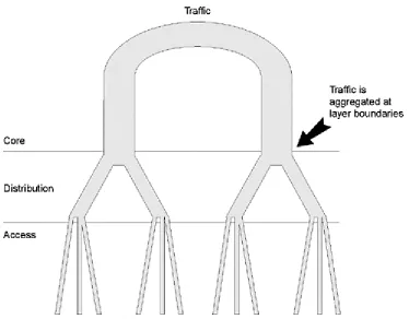
There are generally three layers defined within a hierarchical network. As indicated in Figure 1-1, each layer has a specific design goal:
• The network core forwards traffic at very high speeds; the primary job of a device in the core of the network is to switch packets.
• The distribution layer summarizes routes and aggregates traffic. • The access layer feeds traffic into the network, performs network entry
control, and provides other edge services.
Now that you know the names of the layers, step back and look at how they relate to the fundamental design principles previously outlined. The following are two restated fundamental design principles. The next task is to see if they fit into the hierarchical model.
• The area affected by a topology change in the network should be bound so that it is as small as possible.
• Routers (and other network devices) should carry the minimum amount of information possible.
You can achieve both of these goals through summarization, and summarization is done at the distribution layer. So, you generally want to bound the convergence area at the distribution layer.
For example, a failing access layer link shouldn't affect the routing table in the core, and a failing link in the core should produce minimal impact on the routing tables of access layer routers.
Figure 1-2 Traffic Aggregation and Route Summarization
at Layer Boundaries
The one major weakness inherent in hierarchical network design is that it implies (or creates) single points of failure within the physical layer. The stronger the
hierarchical model, the more likely you are to find places where a single device or a broken link can cause major havoc. Of course, if you don't like havoc, your network must have some measure of redundancy to compensate for this weakness. We'll cover this in Chapter 3,
The Network Core
The core of the network has one goal: switching packets. Like engines running at warp speed, core devices should be fully fueled with dilithium crystals and running at peak performance; this is where the heavy iron of networking can be found. The following two basic strategies will help accomplish this goal:
• No network policy implementation should take place in the core of the network.
• Every device in the core should have full reachability to every destination in the network.
No Policy Implementation
To apply this policy, the network administrator can apply the following configurations to both routers:
1. Build a filter to separate the traffic: 2.
3. access-list 150 permit tcp any eq telnet any 4. access-list 150 permit tcp any any eq telnet 5.
The first line in this access-list selects any TCP traffic destined to the Telnet port; the second one selects any TCP traffic with the Telnet port as its source.
6. Build a policy: 7.
8. route-map telnetthroughframe permit 10 9. match ip address 150
10. set ip next-hop 192.168.10.x 11.
• Perform other edge functions
Access layer devices interconnect the high speed LAN links to the wide area links carrying traffic into the distribution layer. Access layer devices are the visible part of the network; this is what your customers associate with "the network."
Feeding Traffic into the Network
It's important to make certain the traffic presented to the access layer router doesn't overflow the link to the distribution layer. While this is primarily an issue of link sizing, it can also be related to server/service placement and packet filtering. Traffic that isn't destined for some host outside of the local network shouldn't be forwarded by the access layer device.
Never use access layer devices as a through-point for traffic between two distribution layer routers—a situation you often see in highly redundant networks. Chapter 3 covers avoiding this situation and other issues concerning access layer redundancy.
Controlling Access
Since the access layer is where your customers actually plug into the network, it is also the perfect place for intruders to try to break into your network. Packet filtering should be applied so traffic that should not be passed upstream is blocked, including packets that do not originate on the locally attached network. This prevents various types of attacks that rely on falsified (or spoofed) source addresses from originating on one of these vulnerable segments. The access layer is also the place to configure packet filtering to protect the devices attached to the local segment from attacks sourced from outside (or even within) your network.
Access Layer Security
While most security is built on interconnections between your network and the outside world, particularly the Internet, packet level filters on access layer devices regulating which traffic is allowed to enter your network can enhance security tremendously.
For example, in the network in Figure 1-4, you need to apply filters on the access layer router to provide basic security.
The basic filters that should be applied are
• No spoofing
• No broadcast sources • No directed broadcast
No Spoofing
In Figure 1-4, only packets sourced from 10.1.4.0/24 should be permitted to pass through the router.
No Broadcast Sources
The broadcast address 255.255.255.255 and the segment broadcast address 10.1.4.255 are not acceptable source addresses and should be filtered out by the access device.
No Directed Broadcast
A directed broadcast is a packet that is destined to the broadcast address of a segment. Routers that aren't attached to the segment the broadcast is directed to will forward the packet as a unicast, while the router that is attached to the segment the broadcast is directed to will convert the directed broadcast into a normal
broadcast to all hosts on the segment.
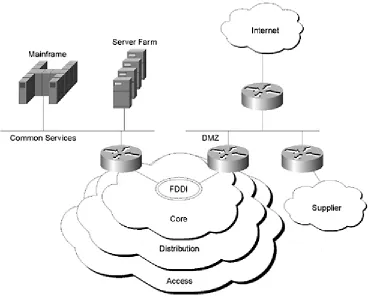
Where these services are connected depends on network topology issues (such as addressing and redundancy, which will be covered in Chapters 2 through 4 in more detail), traffic flow, and architecture issues. In the case of connections to external routing domains, it's almost always best to provide a buffer zone between the external domain and the network core. Other common services, such as mainframes and server farms, are often connected more directly to the core.
Figure 1-5 illustrates one possible set of connections to common services. All external routing domains in this network are attached to a single DMZ, and high-speed devices, which a large portion of the enterprise must access, are placed on a common high-speed segment off the core.
Figure 1-5 Connections to Common Services
One very strong reason for providing a DMZ from the perspective of the physical layer is to buffer the traffic. A router can have problems with handling radically different traffic speeds on its interfaces—for example, a set of FDDI connections to the core feeding traffic across a T1 to the Internet. Other aspects of connecting to common services and external routing domains will be covered in Chapters 2 through 4.
Summary
Case Study: Is Hierarchy Important in Switched
Networks?
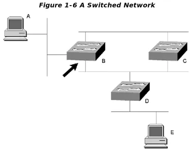
Switched networks are flat, so hierarchy doesn't matter, right? Well, look at Figure 1-6 and see if this is true or not.
Figure 1-6 A Switched Network
Assume that Switch C becomes the root bridge on this network. The two networks to which both Switches B and C are connected will be looped if both switches forward on both ports. Because the root bridge never blocks a port, it must be one of the two ports on Switch B.
If the port marked by the arrow on Switch B is blocking, the network may work fine, but the traffic from Workstation E to Workstation A will need to travel one extra switch hop to reach its destination.
Because Switch B is blocking on one port, the traffic must pass through Switch B, across the Ethernet to Switch C, and then to Switch A. If Switch B were to block the port connected to the other Ethernet between it and Switch C, this wouldn't be a problem.
12: Why is optimum routing so important in the core?
13: What are the primary goals of the distribution layer?
14: What strategies are used in the distribution layer to achieve its goals?
Chapter 2. Addressing & Summarization
Now that you've laid the groundwork to build your network, what's next? Deciding how to allocate addresses. This is simple, right? Just start with one and use them as needed? Not so fast! Allocating addresses is one of the thorniest issues in network design.
If you don't address your network right, you have no hope of scaling to truly large sizes. You might get some growth out of it, but you will hit a wall at some point. This chapter highlights some of the issues you should consider when deciding how to allocate addresses.
Allocating addresses is one of the thorniest issues in network design because:
• Address allocation is generally considered an administrative function, and the impact of addressing on network stability is generally never considered. • After addresses are allocated, it's very difficult to change them because
individual hosts must often be reconfigured.
In fact, poor addressing contributes to almost all large-scale network failures. Why? Because routing stability (and the stability of the routers) is directly tied to the number of routes propagated through the network and the amount of work that must be done each time the topology of the network changes. Both of these factors are impacted by summarization, and summarization is dependent on addressing (see Figure 2-1). See the section "IP Addressing and Summarization" later in this chapter for an explanation of how summarization works in IP.
Figure 2-1. Figure 2-1 Network Stability Is Dependent on
Topology, Addressing, and Summarization
Addressing should, in reality, be one of the most carefully designed areas of the network. When deciding how to allocate addresses, keep two primary goals in mind:
• Controlling the size of the routing table
The primary tool for accomplishing these goals is summarization. It is necessary to come back to summarization again because it is the fundamental tool used to achieve routing stability.
Summarization
Chapter 1, "Hierarchical Design Principles," stated that network stability is dependent, to a large degree, on the number of routers affected by any change. Summarization hides detailed topology information, bounding the area affected by changes in the network and reducing the number of routers involved in convergence.
In Figure 2-2, for example, if the link to either 10.1.4.0/24 or 10.1.7.0/24 were to fail, Router H would need to learn about these topology changes and participate in convergence (recalculate its routing table). How could you hide information from Router H so that it wouldn't be affected by changes in the 10.1.4.0/24, 10.1.5.0/24, 10.1.6.0/24, and 10.1.7.0/24 links?
Figure 2-2 Hiding Topology Details from a Router
Remove detailed knowledge of the subnets behind Router G from Router H's routing table. If any one of these individual links behind Router G changes state, Router H won't need to recalculate its routing table. Summarizing these four routes also reduces the number of routes with which Router H must work; smaller routing tables mean lower memory and processing requirements and faster convergence when a topology change affecting Router H does occur.
IP Addressing and Summarization
IP addresses consist of four parts, each one representing eight binary digits (bits), or an octet. Each octet can represent the numbers between 0 and 255, so there are 232, or 4,294,967,296 possible IP addresses.
To provide hierarchy, IP addresses are divided into two parts: the network and the host. The network portion represents the network the host is attached to; this literally represents a wire or physical segment. The host portion uniquely identifies each host on the network. The IP address is divided into these two parts by the mask (or the subnet mask). Each bit in the IP address, where the corresponding bit in the mask is set to one, is part of the network address. Each bit in the IP address, where the corresponding bit in the mask is set to zero, is part of the host address.
For example, Figure 2-3 shows 172.16.100.10 converted to binary format.
Figure 2-3 IP Addressing in Binary Format
Next, use a subnet mask of 255.255.240.0; the binary form of this subnet mask is shown in Figure 2-4.
Figure 2-4 IP Subnet Mask in Binary Format
By performing a logical AND over the subnet mask and the host address, you can see what network this host is on, as shown in Figure 2-5.
The number of bits set in the mask is also called the prefix length and is represented by a /xx after the IP address. This host address could be written as either
172.16.100.10 with a mask of 255.255.240.0 or as 172.16.100.10/20. The network this host is on could be written 172.16.96.0 with a mask of 255.255.240.0 or as 172.16.96.0/20. Because the network mask can end on any bit, there is a confusing array of possible networks and hosts.
Summarization is based on the ability to end the network mask on any bit; it's the use of a single, short prefix advertisement to represent a number of longer prefix destination networks.
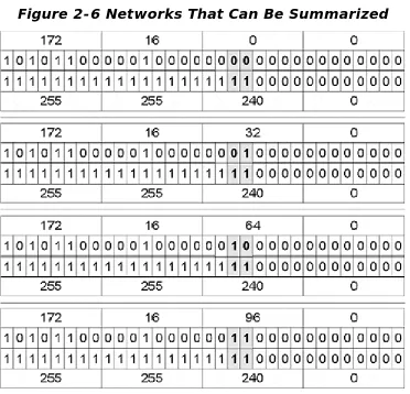
For example, assume you have the IP networks in Figure 2-6, all with a prefix length of 20 bits (a mask of 255.255.240.0).
Figure 2-6 Networks That Can Be Summarized
You can see that the only two bits that change are the third and fourth bits of the third octet. If you were to somehow make those two bits part of the host address portion rather than the network address portion of the IP address, you could represent these four networks with a single advertisement.
172.16.0.0/18, which includes all four of these networks. The prefix length has been shortened in Figure 2-7 as an example.
Figure 2-7 Summarized Network
It's possible to summarize on any bit boundary, for example:
10.100.12.0/25 and 10.100.12.128/25 = 10.100.12.0/24
10.20.0.0/16 and 10.21.0.0/16 = 10.20.0.0/15
172.16.24.0/27 through 172.16.24.96/27 = 172.16.24.0/25
192.168.32.0/24 through 192.168.63.0/24 = 192.168.32.0/19
This last example is commonly called a classless interdomain routing (CIDR) block because it is a supernet of Class C addresses.
Where Should Summarization Take Place?
When deciding where to summarize, follow this rule of thumb: Only provide full topology information where it's needed in the network. In other words, hide any information that isn't necessary to make a good routing decision.
For example, routers in the core don't need to know about every single network in the access layer. Rather than advertising a lot of detailed information about individual destinations into the core, distribution layer routers should summarize each group of access layer destinations into a single shorter prefix route and advertise these summary routes into the core.
Likewise, the access layer routers don't need to know how to reach each and every specific destination in the network; an access layer router should have only enough information to forward its traffic to one of the few (most likely two) distribution routers it is attached to. Typically, an access layer router needs only one route (the default route), although dual-homed access devices may need special consideration to reduce or eliminate suboptimal routing. This topic will be covered more thoroughly in Chapter 4, "Applying the Principles of Network Design."
routers can dramatically reduce the amount of information these routers must deal with.
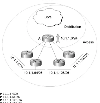
Look at Figure 2-8 for a more concrete example. Router A, which is in the distribution layer, is receiving advertisements for:
Figure 2-8 Summarizing from the Distribution Layer into
the Core
• 10.1.1.0/26 • 10.1.1.64.26 • 10.1.1.128/26 • 10.1.1.192/26
Router A is, in turn, summarizing these four routes into a single destination, 10.1.1.0/24, and advertising this into the core.
Note that all the addresses in a range don't need to be used to summarize that range; they just can't be used elsewhere in the network. You could summarize 10.1.1.0/24, 10.1.2.0/24, and 10.1.3.0/24 into 10.1.0.0/16 as long as 10.1.4.0 through 10.1.255.255 aren't being used.
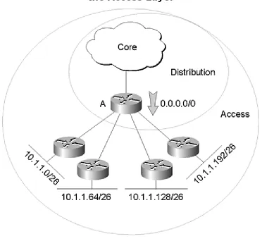
Figure 2-9 is an example of a distribution layer router summarizing the routing information being advertised to access layer devices. In Figure 2-8, the entire routing table on Router A has been summarized into one destination, 0.0.0.0/0, which is called the default route.
Figure 2-9 Summarizing from the Distribution Layer into
the Access Layer
Because this default route is the only route advertised to the access layer routers, a destination that becomes unreachable in another part of the network won't cause these access layer routers to recompute their routing tables. In other words, they won't participate in convergence.
Strategies for Successful Addressing
You can allocate addresses in four ways:
• First come, first serve— Start with a large pool of addresses and hand them out as they are needed.
• Politically— Divide the available address space up so every organization within the organization has a set of addresses it can draw from.
• Geographically— Divide the available address space up so that each of the organization's locations has an office that has a set of addresses it will draw from.
• Topologically— This is based on the point of attachment to the network. (This may be geographically the same on some networks.)
First Come, First Serve Address Allocation
Suppose you are building a small packet switching network (one of the first) in the 1970s. You don't think this network will grow too much because it's restricted to only a few academic and government organizations, and it's experimental. (This
prototype will be replaced by the real thing when you're done with your testing.)
No one really has any experience in building networks like this, so you assign IP addresses on a first come, first serve basis. You give each organization a block of addresses, which seems to cover their addressing needs. Thus, the first group to approach the network administrators for a block of addresses receives 10.0.0.0/8, the second receives 11.0.0.0/8, and so on.
This form of address allocation is a time -honored tradition in network design; first come, first serve is, in fact, the most common address assignment scheme used. The downside to this address allocation scheme becomes apparent only as the network becomes larger. Over time, a huge multinational network could grow to look like the Internet—a mess in terms of addressing. Next, look at why this isn't a very good address allocation scheme.
In Figure 2-10, the network administrators have assigned addresses as the departments have asked for them.
This small cross-section of their routers shows:
• Router A has two networks connected: 10.1.15.0/24 and 10.2.1.0/24 • Router B has two networks connected: 10.2.12.0/24 and 10.1.1.0/24 • Router C has two networks connected: 10.1.2.0/24 and 10.1.41.0/24 • Router D has two networks connected: 10.1.40.0/24 and 10.1.3.0/24
There isn't any easy way to summarize any of these network pairs into a single destination, and the more you see of the network, the harder it becomes. If a network addressed this way grows large enough, it will eventually have stability problems. At this point, at least eight routes will be advertised into the core.
Addressing by the Organizational Chart (Politically)
Now, start over with this network. Instead of assigning addresses as the various departments asked for them, the network administrators decided to put some structure into their addressing scheme; each department will have a pool of addresses to pull networks from:
• Headquarters: 10.1.0.0/16 • Research: 10.2.0.0/16 • Quality: 10.3.0.0/16 • Sales: 10.4.0.0/16
• Manufacturing: 10.5.0.0/16
With this addressing scheme in place, the network now looks like Figure 2-11.
Now, there may be some opportunities for summarization. If 10.1.3.0/24 isn't assigned, it might be possible to summarize the two headquarters networks into one advertisement. It's not a big gain, but enough little gains like this can make a big difference in the stability of a network.
In general, though, this addressing scheme leaves you in the same situation as the first come, first serve addressing scheme —the network won't scale well. In Figure 2-11, there will still be at least seven or eight routes advertised into the core of the network.
Addressing Geographically
Once again, you can renumber this network; this time assign addresses based on the geographic location. The resulting network would look like Figure 2-12.
Figure 2-12 Addressing by Geographic Location
Just working with the networks illustrated here, you can summarize the two US networks, 10.4.1.0/24 and 10.4.2.0/24 into 10.4.0.0/16, so Router A can advertise a single route into the core. Likewise, you can summarize the two Japan routes,
10.2.1.0/24 and 10.2.2.0/24, into 10.2.0.0/16, and Router D can advertise a single route into the core.
London, however, presents a problem. London Research, 10.1.2.0/24, is attached to Router C, and the remainder of the London offices are attached to Router B. It isn't possible to summarize the 10.1.x.x addresses into the core because of this split.
Addressing by Topology
The most effective way of making certain that routes can be summarized is to assign addresses based on the router to which the network is attached or, rather, the topology of the network. Addressing this network based on the topology results in Figure 2-13.
Figure 2-13 Topological Address Assignment
Summarization can now be configured easily on Router A, Router B, Router C, and Router D, reducing the number of routes advertised into the rest of the network to the minimum possible. This is easy to maintain in the long term because the configurations on the routers are simple and straightforward.
Topological addressing is the best assignment method for ensuring network stability.
Combining Addressing Schemes
One complaint about assigning addresses topologically is it's much more diffic ult to determine any context without some type of chart or database—for example, the department to which a particular network belongs. Combining topological addressing with some other addressing scheme, such as organizational addressing, can
minimize this.
FE80::172.16. 10.4
Other differences in addressing are not readily apparent; for example, in IPv4, the class of an address is determined by the first few bits in the address:
0 Class A (0.0.0.0 through 126.255.255.255)
10 Class B (128.0.0.0 through 191.255.255.255)
110 Class C (192.0.0.0 through 223.255.255.255)
1110 Class D (multicast, 224.0.0.0 through 239.255.255.255)
1111 Class E (experimental, 240.0.0.0 through 255.255.255.255)
In IPv6, the first few bits of the address determine the type of IP address:
010—service provider allocated unicast addresses (4000::0 through 5FFF:FFFF:FFFF:FFFF:FFFF:FFFF:FFFF:FFFF)
100—geographically assigned unicast addresses (8000::0 through 9FFF:FFFF:FFFF:FFFF:FFFF:FFFF:FFFF:FFFF)
1111 1110 10—link local addresses (FE80::0 through FEBF:FFFF:FFFF:FFFF:FFFF:FFFF:FFFF:FFFF)
1111 1110 11—site local addresses (FEC0::0 through FEFF:FFFF:FFFF:FFFF:FFFF:FFFF:FFFF:FFFF)
1111 1111—multicast addresses (FF00::0 through all F's)
There are also some special addresses in IPv6:
0::0—unspecified
0::1.1.1.1 through 0::255.255.255.255—IPv4 addresses
0::0001—loopback
Note that there is no broadcast address defined any longer; the all hosts multicast is used instead. There are many other differences between IPv4 and IPv6—everything from packet formats to how a host determines its address. Several books and RFCs cover IPv6; you should consult them to learn more about these differences.
General Principles of Addressing
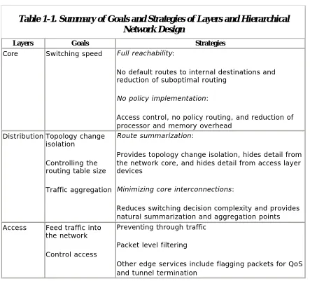
Addressing and summarization are critical to a stable network. Addressing must be carefully planned to allow for summarization points; summarization, in turn, hides information, promoting network stability. These principles are covered in Table 2-1 for future reference.
Table 2-1. Summarization Points and Strategies
Summarization Points Strategies
Distribution layer to core
Summarize many access layer destinations into a few advertisements into the core.
Hide detailed distribution layer and access layer topology information from the core.
Distribution layer to
access layer Summarize entire network topology down to a very small set of advertisements to access layer devices (default route if possible).
Provide route to nearest distribution layer router with access to the core.
Hide topology of core and distribution layer from access layer devices.
The general principles of addressing are
• Use a large address space if possible • Leave room for future growth
Table 2-2. Summary of Addressing Schemes
Addressing Scheme Advantages and Disadvantages
First come, first serve
Doesn't require any planning.
Almost always results in an impossible to manage network. Politically Requires minimal planning.
Easy to resolve an address to a particular part of the organization.
If the organization is subdivided geographically, this scheme works well; otherwise, it can produce a network that will not scale.
Geographically Requires planning.
Enables some degree of summarization. Topologically Requires planning.
Enables summarization, drastically reduces routing table sizes in the core in large-scale networks.
Scales well.
Generally easy to configure and maintain.
Allocation schemes can sometimes be combined to provide a solution that is easy to manage and scale.
Case Study: Default Routes to Interfaces
From time to time, routers are configured with a default route pointing to an interface. In some situations, this is fine, but in others, this can be disastrous. The problems have to do with the link type, ARP, and proxy ARP, which is not well understood.
In Figure 2-15, Router A has a default route configured out interface Ethernet 0:
ip route 0.0.0.0 0.0.0.0 Ethernet 0
Router B has a default route configured out interface serial 0:
The complaint is that Router A seems to have extremely high processor utilization and is providing sluggish performance at best. Examine the actions of Router B when ws2, which is configured to use Router B as its default gateway, sends a packet to the Internet. Seeing that the destination it seeks is not on the local segment, ws2 sends the packet to its default gateway; when B receives the packet, it examines its routing table to find a forwarding entry for the destination. Assuming it has no entry, it will forward the packet along its default route, which is pointing to its serial
interface.
Figure 2-15 Default Route to a Broadcast Interface
Given that the serial interface on Router B is attached to a point-to-point circuit, there is no place for Router B to forward the packet other than the other end of the circuit. Router B's decision is clear-cut: place the packet on the point-to-point circuit.
Now, consider what takes place when ws1 sends a packet that is destined to some host on the Internet. Noting the final destination is not on its local network, ws1 forwards the packet to its default gateway (in this case, Router A). When Router A receives the packet, it examines its forwarding table for a route to this destination and decides to use its default route, which points to its Ethernet 0 port.
The problem for Router A is this: Ethernet 0 is connected to a multi-access link, and Router A doesn't know which next hop to use to get to the destination in question (because the route points to the interface rather than a specific IP address). So, Router A will ARP the Ethernet segment. Essentially, Router A believes that everything for which it does not have a specific route is actually connected to its Ethernet 0 port.
Router B will receive the ARP request and examine its routing table to see if it knows how to reach this destination. Router B finds a default route in its table, which will do nicely, so it replies to Router A's ARP request. Router A installs an ARP cache entry for this destination IP address bound to Router B's Ethernet address. Router B's ARP reply is called a proxy ARP because Router B is essentially proxying for every
10.1.4.1 (the inside address) appears as 127.10.1.10 (the outside address) on the Internet after translation. On Cisco routers, 10.1.4.1 is called the inside local
address, 127.10.1.10 is called the inside global address, and 109.10.1.4 is called the outside global address.
The configuration of the router running NAT (Router A) may look like this:
ip nat pool tothenet 127.10.1.10 127.10.1.10 prefix-length 24 ip nat inside source list 1 pool tothenet
!
interface Eternet 0 ip nat inside !
interface Serial 0 ip nat outside !
access-list 1 permit 10.0.0.0 0.255.255.255
This one-to-one translation of inside local addresses to inside global addresses is useful, but it doesn't help much when you have a large number of hosts on the inside network and only a few addresses to use on the outside.
Because it's common to have a large number of inside addresses translated into a much smaller pool of outside addresses, most NAT implementations allow a finer granularity of address assignment called Port Address Translation (PAT), or overloading.
In PAT, for each session the inside host initiates, it's assigned a port number on the inside global (or translated) address. This allows about 32,000 simultaneous sessions from the inside to the outside using one inside global address. See Figure 2-18 for an example of PAT translated address.
Assuming that each inside host is likely to have 10 open sessions to outside hosts at any time, about 3,000 inside hosts could be represented by one outside address. The configuration on Router A (refer to Figure 2-16) may look like this:
ip nat pool tothenet 127.10.1.10 127.10.1.10 prefix-length 30 ip nat inside source list 1 pool tothenet overload
!
interface Ethernet 0 ip nat inside
!
interface Serial 0 ip nat outside !
access-list 1 permit 10.0.0.0 0.255.255.255.
Cisco routers don't assign the port on the inside global address randomly; the router assigns ports from a series of pools. The ranges are
1–511
512–1023
1024–4999
5000–65535
If the inside hosts used port 500 as its source port, for instance, the router will choose a port between 1 and 511 for the source port when it translates the address.
Review
1: Why is it difficult to change addresses after they've been assigned?
2: Why is address allocation so closely tied to network stability?
3: What are the goals you should keep in mind when allocating addresses?
5: How does hiding topology details improve stability?
6: Where should summarization take place?
7: What is the one case where access layer devices should be passed more than a default route? Why?
8: An IP address can be divided into two parts; what are they?
9: What is the prefix length of a network?
10: Find the longest prefix summary for these addresses.
• Set A: 172.16.1.1/30, 172.16.1.5/30, 172.16.1.9/30, 172.16.1.14/30 • Set B: 10.100.40.14/24, 10.100.34.56/24, 10.100.59.81/24
• Set C: 172.18.10.10/23, 172.31.40.8/24, 172.24.8.1/22, 172.30.200.1/24
• Set D: 192.168.8.10/27, 192.168.60.14/27, 192.168.74.90/27, 192.168.101.48/27
11: Explain the effects of pointing a default route to a broadcast network interface.
12: What does a pair of colons with no numbers in between signify in an IPv6 address? How many times can you use this symbol in an address?
13: Explain the difference between Network Address Translation (NAT) and Port Address Translation (PAT).
14: Address the network depicted in Figure 2-19 by
• Organization
• Geographical location • Topology
Chapter 3. Redundancy
A single point of failure is any device, interface on a device, or link that can isolate users from the services they depend on if it fails. Networks that follow a strong, hierarchical model tend to have many single points of failure because of the emphasis on summarization points and clean points of entry between the network layers. For example, in a strict hierarchical network, such as the one depicted in Figure 3-1, every device and every link is a single point of failure.
Figure 3-1. Figure 3-1 Every Device and Link in This
Network Is a Single Point of Failure
However, this network will be safe if it's protected by dial backup. Redundancy can save the day.
Redundancy provides alternate paths around these failure points, providing some measure of safety against loss of service. Be careful, though: Redundancy, if not designed and implemented properly, can cause more trouble than it is worth. Each redundant link and each redundant connection point in a network weakens the hierarchy and reduces stability.
If your core routers aren't all in one building (or on one campus), your options become more limited (and more expensive, of course). With larger scale core networks, three competing goals must be balanced for good design:
• Reducing hop count • Reducing available paths
• Increasing the number of failures the core can withstand
The following sections depict some designs that illustrate these principles.
Ring Core Design
Ring core designs, such as the one pictured in Figure 3-3, are relatively common; they are easy to design and maintain (for the most part). Note that this ring core is the type formed using multiple point-to-point links to interconnect multiple routers. There are some designs that rely on a ring at the lower (physical) layer. (To the routers, they appear to be a single high-speed broadcast network—see the following "Redundant Fiber Ring Technologies" section.)
Following are the properties of the ring core design shown in Figure 3-3:
• There are two paths to any given destination from every core device. • A packet crosses a maximum of four hops with the entire core intact.
• Losing a single link increases the maximum number of hops through the core to six.
• Losing any two links isolates at least one piece of the network.
Ring core designs do well with reducing the number of available paths while still providing redundancy, but they fail miserably at the other goals.
The number of possible routes through the network is low during normal operation, but the number of hops a packet may have to cross with a single link down is unreasonable. A two-hop path to reach a server could become a six-hop path if a single link fails. A big jump like this can cause session timeouts and other problems.
There's not a lot of redundancy afforded with a ring design; losing any two links on the core will isolate some piece of the network. There are ways of circumventing this, but they involve backups of backups, or other types of kludges, which will end up being difficult to maintain and scale in the long term. It's better to design it right the first time.
Redundant Fiber Ring Technologies
Network (SONET), also known as Synchronous Digital Hierarchy (SDH). This technology was standardized by the CCITT as G.707, G.708, and G.709.
SONET networks consist of a pair of fiber optic links between each node on the ring. The first fiber is normally used to pass data at speeds of up to OC-48 (2488.32 Mbps). The second fiber is used as a redundant path. If the first fiber is cut or becomes otherwise unusable, traffic is automatically shifted to the second fiber.
FDDI is another technology that provides this sort of redundancy with two rings on which the data rotates in opposite directions (two counter rotating rings). If the fiber fails at any point between two dual attached nodes (devices that are attached to both rings), the ring will wrap, healing the break.
These technologies provide the redundancy at Layer 2 in the OSI model, resolving many of the issues with providing redundancy at the network layer. This type of technology could be emulated with normal point-to-point technologies by installing two links between each device in the core ring and only advertising the backup path when the primary path becomes unusable.
These methods do not, however, provide redundancy for the devices on the core; they only provide redundancy for the links between the devices. Redundancy for device failures almost always requires a network layer solution or Layer 2 switching.
Full Mesh Core Design
Full mesh designs, where every core router has a connection to every other core router, provide the most redundancy possible. The design in Figure 3-4 provides the following:
• A large number of alternate paths to any destination. • A two hop path to any destination under normal use.
• A four hop maximum path in the worst case scenario (multiple links down with full connectivity).
• Exceptional redundancy; because every router has a link to every other router, this network would have to lose at least three links before any destination became unreachable.
Full mesh designs do well in the hop count and maximum redundancy areas. Unfortunately, full mesh designs can provide too much redundancy in larger networks, forcing a core router to choose between a large number of paths to any destination, which increases convergence times.
In Figure 3-4, Router A has five paths to Router C:
• Router A to Router C
• Router A to Router B to Router C • Router A to Router D to Router C
• Router A to Router B to Router D to Router C • Router A to Router D to Router B to Router C
Figure 3-5 Routers Versus Paths in a Full Mesh
Full mesh networks can be expensive because of the number of links required. These networks also need a lot of configuration management because there are many places to make mistakes when implementing a change. It's difficult to engineer traffic on a full mesh network; the path that traffic normally takes can be confusing, making it difficult to decide how to size physical links (see "Case Study: What's the Best Route?" at the end of this chapter for further information).
Partial Mesh Core Design
Partial mesh cores tend to be a good compromise in hop count, redundancy, and the number of paths through the network. In Figure 3-6, there are four paths between any two points on the network, for example, between Router A and Router F:
• Router A to Router D to Router F • Router A to Router C to Router F
• Router A to Router D to Router E to Router C to Router F • Router A to Router C to Router B to Router D to Router F
There is a clear difference in the lengths of the four paths available, which means only the two equal length paths will be used at any time for normal traffic flow. No more than three hops will be required to traverse the network during normal operation; if any single link fails, the maximum number of hops to traverse the network will increase to four. These low hop counts tend to stay low as a partial mesh core grows.
The redundancy provided by a partial mesh design is good, as well: The network in Figure 3-6 provides full connectivity with three links down as long as no single router loses both of its connections to the mesh.
The major drawback for partial mesh cores is that some routing protocols don't handle multipoint partial mesh designs well, so it's much better to stick with point-to-point links of some type in the core (such as point-point-to-point subinterfaces for ATM or Frame Relay).
Routing Protocols and Partial Mesh Technologies
interfaces typically provide this type of connectivity, called point-to-multipoint or nonbroadcast multi-access (NBMA).
Figure 3-7 Routing Protocols in a Partial Mesh Topology
By default, OSPF treats NBMA networks as if they were broadcast links, which means a designated router will be elected. (See Appendix A, "OSPF Fundamentals," for more information on designated routers.)
This isn't really a broadcast network, though. Because Router A has direct connections to both Router B and Router C, Router A will receive any broadcasts Router B or Router C send. Router B, however, won't receive any broadcasts Router C transmits because there is no link between them; likewise, Router C won't receive any broadcasts transmitted by Router B.
For OSPF, this means only Router A will receive Router B's and Router C's Hellos; Router B won't receive Router C's Hellos, and Router C won't receive Router B's Hellos. Router A, Router B, and Router C will all have different views of the designated router election process. Router A might think that Router B is the
Dual Homing to the Core
In Figure 3-8, Router A has two connections to the core through separate routers. While this provides very good redundancy—the loss of a single core router or a single link won't make any destinations behind Router A unreachable —it can also create some problems.
Figure 3-8 Dual Homing in the Distribution Layer
If Router A were connected only to one core router, Router D would have two paths to 172.16.0.0/16:
• Router D to Router B to Router A
• Router D to Router C to Router B to Router A
With Router A dual-homed to the core, Router D has four paths to this destination:
• Router D to Router C to Router A • Router D to Router B to Router A
Dual homing Router A to the core effectively doubles the number of paths available to 172.16.0.0/16 in the core. This doubling of possible routes for every dual-homed distribution layer router slows network convergence.
It's sometimes possible to force the metric or cost of one of the two paths to be worse so that traffic will normally flow over only one link. The number of paths is still doubled, so this isn't a very effective solution for advanced routing protocols. A better solution would be to only advertise 172.16.0.0/16 over one link unless that link becomes unusable. Conditional advertisement and floating static routes can be used to only advertise a route when necessary.
Dual homing also presents one other problem: If the link between Router B and Router C goes down, Router A could be effectively drawn into a core role, passing transit traffic between Router B and Router C. This may be a valid design if it's anticipated and planned for, but it's generally not. The easiest way to prevent this from occurring is to configure Router D so it doesn't advertise routes learned from Router C back to Router B, and so it doesn't advertise routes learned from Router D back to Router C.
Redundant Links to Other Distribution Layer Devices
Installing links between distribution layer routers to provide redundancy has the following drawbacks (see Figure 3-9):
• Doubling the core's routing table size— As was discussed when looking at dual homing distribution layer devices to the core, adding the link between Router A and Router B in Figure 3-9 doubles the size of the core routing table because Router D now has paths through both Router A and Router C to the 172.16.0.0/16 network.
• Possible use of the redundant path for traffic transiting the core — If the link between Router D and Router C fails in Figure 3-9, it's possible that Router D could begin forwarding traffic to Router A, which is destined
someplace beyond Router C, rather than forwarding the traffic to Router E. Router A and Router B can be effectively drawn into a core routing role. • Preferring the redundant link to the core path— Distribution layer
routers may end up preferring the redundant path through the distribution layer, rather than the path through the core. In Figure 3-9, it's possible that Router B would prefer the redundant link to the path through the core to reach the 172.16.0.0/16 network.
Access Redundancy
The access layer presents many of the same challenges and issues as the distribution layer, and it also shares some of the same strategies for resolving these drawbacks. Dual homing access layer devices are the most common way of providing
redundancy to remote locations, but it's also possible to interconnect access layer devices to provide redundancy.
In Figure 3-10, Router G and Router H are access layer routers that are dual-homed with the backup circuit connected to different branches of the distribution layer. If these redundant links are actually constantly up and carrying traffic, the number of paths between 10.2.1.0/24 and 10.1.1.0/24 is excessive:
Figure 3-10 Access Layer Redundancy—Dual Homing
through Different Distribution Branches
• Router H to Router F to Router B to Router A to Router C to Router G • Router H to Router F to Router B to Router E to Router G
With each addition of a dual-homed access layer router, things get worse. This plethora of paths causes major problems in the core; the size of the routing table in the c ore will mushroom. This is the general rule: If the redundant link crosses the boundary of a distribution layer branch, it should not be advertised as a normal path.
Another option to provide access layer redundancy (and another illustration of the general rule above) is to provide links between the access layer routers themselves. In Figure 3-11, this saves one link, and it also reduces the number of paths between 10.1. 1.0/24 and 10.2.1.0/24 down to two. If access layer redundancy is provided using links between access devices, it's important to provide enough bandwidth to handle the traffic from both remote sites toward the core.
Figure 3-11 Redundancy through Interconnected Access
Layer Devices
Either of these solutions would work well as long as the redundant route is not advertised until needed, so traffic won't normally flow across the redundant link. Dial-on-demand circuits work well for these types of applications.
Figure 3-12 Access Layer Redundancy through the Same
Distribution Layer Branch
It's still possible for packets traveling from Router C to Router D to pass through Router G, but this can be remedied with route filtering. Router G and Router H should only advertise the networks below them in the hierarchy. In Figure 3-12, this is 10.1.1.0/24 for Router G and 10.2.1.0/24 for Router H. If correct filtering is installed in Router G, Router C will not learn any paths through Router D by way of Router G.
One way to get around all of the problems associated with dual homing is to use dial backup. There are two sections at the end of this chapter, "Case Study: Dial Backup with a Single Router" and "Case Study: Dial Backup with Two Routers," that cover these options.
Connections to Common Services
network these common services are attached to. Side A of Figure 3-13 illustrates this single point of failure.
Figure 3-13 Redundancy to Common Shared Resource,
Such as a Server Farm
In the network illustrated by Side B of Figure 3-13, the server farm has been connected to two core routers, so the failure of a single router will not affect the reachability of the server farm.
In a similar way, Figure 3-14 illustrates multiple connections to an external routing domain for redundancy. In this case, the links to the external routing domain are directly attached to the core.
Providing redundancy for links through a DMZ is more complicated because there are two points of failure that need to be considered: the link between the core and the DMZ, and the link between the DMZ and the external domain. Figure 3-15 illustrates an external routing domain attached through a redundant DMZ.
• IGRP: 100 • OSPF: 110 • IS-IS: 115 • RIP: 120 • EGP: 140
• EIGRP External: 170 • BGP Internal: 200 • Unknown: 255
The administrative distance for connected routes cannot be changed, but it can be changed for other protocols. Each of the routing protocol's administrative distances can be changed using the distance command in router configuration mode. The administrative distance for each static route can be set using an option in the ip route command:
ip route 10.1.1.0 255.255.255.0 x.x.x.x 200
The ability to change the administrative distance of a static route this way has led to the concept of a floating static route, which is a static route with a high
administrative distance, typically 200 or above.
These floating statics are useful for backing up primary routes or conditionally advertising a route.
Case Study: Redundancy at Layer 2 Using Switches
It's often possible to build redundancy into a network at the data link layer rather than the network layer. One example of this is the FDDI ring, which has two physical paths between each station on the ring. Another possibility is to use switches running the Spanning-Tree Algorithm to choose between redundant paths.
For example, in the network in Figure 3-16 there are actually eight paths from Router G to the FDDI ring, but Router G would see only two of them. Spanning tree running between Switches C and D would block some ports to eliminate any loops.
Following is an example of one pair of paths through the network. There are two possible paths between Router A and Router E: Router A to Switch C to Router E and Router A to Switch D to Router E, crossing VLAN 1.
Assume that the port which blocks is Switch D's port onto VLAN 1. If Switch C fails, Switch C would recalculate spanning tree and begin forwarding traffic across VLAN 1. The routers wouldn't even know that a network failure had occurred.
If Router E were to fail, Router G would begin using the alternate routed path through Router F to reach the FDDI ring. No single link or equipment failure would cause an outage on this network.
While this example shows LANs (specifically Ethernet VLANs) being used as
intermediate links, it's also possible to use switches to provide redundancy over wide area links, such as Frame Relay or ATM.
When using switched virtual circuits rather than permanent virtual circuits (or in combination with permanent virtual circuits), it's possible to have a mesh of redundant connections between switches that are completely transparent to the routers on the edges of the network cloud. Physical layer redundancy is often easier to implement and can provide faster recovery than providing redundancy at the network layer. It can also be less complicated to maintain and manage.
Physical layer redundancy doesn't provide fallbacks for failure in the routers at the edge, however. Because routers are Layer 3 devices, router redundancy must be provided for at Layer 3 with a routing protocol (or something along the lines of floating static routes).
Case Study: Dial Backup with a Single Router
While BGP is capable of conditional advertisement, most other routing protocols aren't. You need to find a way to advertise backup links only under certain conditions, particularly if they are dial-on-demand, such as ISDN.
Figure 3-17 depicts a common scenario; Router B has a point-to-point link through Serial 0 to Router A, and a dial-on-demand backup link through BRI 0 to Router C. The routing protocol is EIGRP, and Router B is only receiving 0.0.0. 0/0 advertised from Router A (the default route). The network administrator doesn't want the ISDN link up unless the serial link fails.
There are two possibilities for bringing the ISDN dial-on-demand link up when the serial interface fails:
1. Configuring the ISDN link as a backup interface. Configuring an interface as a backup, as the name implies, instructs the router to bring a dial interface up in response to another interface's line state changing to down.
2. Using a combination of floating static routes and a dynamic routing protocol to redirect traffic over the ISDN link.
It's relatively simple to configure the ISDN interface as a backup interface for Serial 0 in Figure 3-17. On Router B:
isdn switch-type basic-ni1 !
interface BRI0
ip address 172.16.10.33 255.255.255.252 encapsulation ppp
interface Serial 0
ip address 172.16.10.29 255.255.255.252 encapsulation frame-relay
!
ip route 0.0.0.0 0.0.0.0 172.16.10.34 200 access-list 101 deny eigrp any any
access-list 101 permit ip any any dialer-list 1 protocol ip list 101
The number at the end of the IP route command indicates an administrative distance. Because Router C would normally have a 0.0.0.0/0 route from Router A through EIGRP, this static route will not normally be used (placed in the routing table). If Router A were lost as an EIGRP neighbor, though, Router C would begin using this static, which points out through the ISDN link.
Once interesting traffic begins to be forwarded out of interface BRI 0 (as defined by
dialer-list 1), the router will begin the ISDN link up. Once the serial link is restored, the 0.0.0.0/0 route learned through EIGRP from Router A should once again be installed in the routing table, and all traffic should be forwarded through the serial interface.
Because EIGRP is not considered interesting traffic, the router will eventually bring the ISDN link down.
Note that in both of these configurations, IP route-cache is disabled on the ISDN interface. It's important that the router not cache any destinations as reachable through the ISDN interface because it will continue sending traffic for those destinations through the ISDN interface, regardless of the state of the serial interface, until the route cache entry times out.
Case Study: Dial Backup with Two Routers
Dial backup using a single router at the remote site still leaves a single point of failure—the router at the remote site. The obvious solution is to install two routers at the remote site, as illustrated in Figure 3-18.
There are two problems with this solution; the first is that hosts on the
172.16.9.0/24 network must set their default gateways to either Router B's or Router D's Ethernet IP address to reach the rest of the network. No matter which one is used, if that router fails completely, all connectivity to this segment will effectively be lost.
The second is Router B must be able to signal Router D that its serial link to Router A has failed.
The first problem can be resolved using Hot Standby Router Protocol (HSRP). HSRP allows Router B and Router D to share a virtual IP address between them with only the active HSRP router accepting (and forwarding) traffic destined to that IP address. Following is an exa mple of how this would work.
On Router B, the configuration is as follows:
interface e0
ip address 172.16.9.2 255.255.255.0 standby ip 172.16.9.1
designs to get around this problem?
13: When dual homing a distribution layer or access layer router, what major problem should you be careful of?
14: When interconnecting distribution or access layer routers to provide redundancy, what issues should you be careful of?
Chapter 4. Applying the Principles of
Network Design
The elements of network design—hierarchy, redundancy, addressing, and summarization—have been addressed in relative isolation up to this point. The following list groups them together:
• Hierarchy— Provides a logical foundation, the "skeleton" on which addresses "hang."
• Addressing— Isn't just for finding networks and hosts; it also provides points of summarization.
• Summarization— The primary tool used to bound the area affected by network changes.
• Stability/Reliability— Provided by bounding the area affected by changes in the network.
• Redundancy— Provides alternate routes around single points of failure. Figure 4-1 shows the traffic and routing table patterns throughout a well-designed hierarchical network. (You may recognize Figure 4-1 because you have seen pieces of it in previous chapters.) Note that the routing table size is managed through summarization; so, no single layer has an overwhelming number of routes, and no single router must compute routes to every destination in the network if a change does occur.
How do you design a network so that the routes and traffic are well-behaved? By managing the size of the routing table. Managing the size of the routing table is critical in large-scale network design.
The primary means of controlling the routing table size in a network is through summarization, which was covered in detail in Chapter 3, "Redundancy."
Summarization is highly dependent on correct addressing. Therefore, the routing table size, summarization, and addressing (the three basics of highly scalable networks) are closely related.
To illustrate these principles, this chapter begins with a network that is experiencing stability problems and "reforms" it to make it stable and scalable. This exercise applies the principles discussed in the first three chapters of this book.
Reforming an Unstable Network
This section of the chapter reforms the network shown in Figure 4-2. Because this is a rather large network, only one small section is tackled at a time. This chapter covers how to implement changes in the topology and addressing, which can
improve this network. Chapter 5, "OSPF Network Design," Chapter 6, "IS-IS Network Design," and Chapter 7, "EIGRP Network Design" address how to implement routing protocols on this network.
This exercise begins with the core of the network and works outward to the distribution and access layers as detailed in the following sections.
Examining the Network Core
As you consider the core of this network, it's good to remember the design goals that you worked through for network cores back in Chapter 1, "Hierarchical Design
Principles." As your primary concerns, focus on switching speed and providing full reachability without policy implementations in the network core.
need to narrow your focus a bit; Figure 4-3 shows only the core and its direct connections.
Figure 4-3 The Network Core
Network traffic in the network illustrated in Figure 4-3 flows between the common services and external connections to and from the HQ VLANs and the networks behind the distribution layer. A diagram of this network traffic reveals that most traffic flows:
• From the networks behind Routers A, C, and D to the networks behind Router E
• From the networks behind Routers A, C, and D to the networks behind Router B
Because there won't be much traffic flowing between Router A and Router C or Router A and Router D, these are the two best links to remove. Removing these two links will reduce the core to a partially- meshed network with fewer paths and more stability. The total number of paths through the core will be cut from 20 to 6, at most, for any particular destination.
Beyond the hyper-redundancy, there are also network segments with hosts connected directly to Router A—the corporate LAN VLAN trunks. Terminating the corporate VLANs directly into Router A means:
• Router A must react to any changes in the status of corporate VLAN.
You do, however, need to summarize the routes advertised from the HQ VLANs anyway. Because the routers within the core are going to have more specific (longer prefix) routes to any destination within the core, everything will work.
Relying on leaked, longer prefixes to provide correct routing is not recommended because the prefixes can be difficult to maintain, and simple configuration mistakes can cause major side effects. But it is useful to consider this option if you are in a position where networks can't be renumbered to summarize correctly.
Figure 4-4 provides an illustration of what the redesigned core from Figure 4-2 looks like after these changes:
Figure 4-4 Redesigned Network Core
• Removing the excessive redundancy in the core by removing two point-to-point links
• Adding a single router between the core and the HQ VLANs to move policy implementation and summarization out of the core
• Renumbering the point-to-point links in the core
Distribution Layer and Access Layer Topology
As you work through the access and distribution area of this network, keep the goals of the layers in mind. The goals for the distribution layer are as follows:
• Control the routing table size by isolating topology changes through summarization.
• Aggregate traffic.
The goals for the access layer are as follows:
• Feed traffic into the network.
• Control access into the network, implement any network policies, and perform other edge services as needed.
Because the design of the distribution and access layers is so tightly coupled, you need to examine them together. Figure 4-5 focuses on the distribution and access layers and the Frame Relay links that connect them. This way you can more easily understand them in context with the discussion that follows.
Figure 4-5 Distribution and Access Layers
These modifications leave a plethora of paths; normally, there are four ways to reach any access layer network from the core. For example, the 172.16.25.0/24 network has the following paths:
• Cloud E, Router A, Core (through 172.16.21.12/30) • Cloud E, Router A, Core (through 10.1.1.26/26) • Cloud M, Router B, Core (through 172.16.21.8/30) • Cloud M, Router B, Core (through the alternate link)
A single failure (for example, Router A) leaves two paths through Router B. A second failure (Frame Relay Cloud M, for example) isolates the remote networks. If the second failure isolates the remote network anyway, why leave in the extra redundancy?
Figure 4-7 shows the network after removing the extra (redundant) links between the core and the distribution layer routers, which leaves two paths between the core and any remote network.
So far, then, you have moved some links around in between the distribution layer and the core to provide better points of summarization. You have also removed some redundancy, which, it turns out, is overkill. The next step is to make any possible changes in addressing in the distribution and access layers to improve stability.
Overhead in Routing Protocols
There are two things engineers yearn for in a good routing protocol: instantaneous convergence and no overhead. Since that is not possible, it is necessary to settle for a low overhead protocol with very fast convergence. But what defines low overhead?
One major component of routing protocol overhead is interruption due to updates. You don't want to use a routing protocol that interrupts every host on the network every 30 seconds with a routing update (like Routing Information Protocol [RIP] does). To combat update overhead, routing protocols attempt to reduce the scope and the frequency of interruptions.
Assume that both Routers A and B are advertising a summary of 172.16.24.0/21, which is the address space from 172.16.24.0 through 172.16.31.0. Therefore, the summary covers the remote network and the links between the access and
distribution layer routers shown in Figure 4-8. Furthermore, assume that Router B is used by the core routers as the preferred path to this summary for whatever reason (link speed, and so forth).
Given these conditions, if the remote router's link onto frame Cloud M fails, all connectivity with the remote network 172.16.25.0/24 will be lost, even though the alternate path is still available. It might be very unlikely, of course, that this could happen, but it is possible and worth considering.
External Connections
This section separately examines the external connections to the network, as was done for the network core and distribution and access layers (see Figure 4-9).
Figure 4-9 External Connections
It only takes a quick look to see that there are too many links between the core of this network and the external networks—three connections to