Chaos, control, and synchronization in some fractional order difference equations

(1)

R E S E A R C H

Open Access

Chaos, control, and synchronization in some

fractional-order difference equations

Amina-Aicha Khennaoui

1

_{, Adel Ouannas}

2

_{, Samir Bendoukha}

3

_{, Giuseppe Grassi}

4

_{, Xiong Wang}

5

_,

Viet-Thanh Pham

6*

_{and Fawaz E. Alsaadi}

7

*_{Correspondence:} [email protected] 6_{Nonlinear Systems and}

Applications, Faculty of Electrical and Electronics Engineering, Ton Duc Thang University, Ho Chi Minh City, Vietnam

Full list of author information is available at the end of the article

Abstract

In this paper, we propose three fractional chaotic maps based on the well known 3D Stefanski, Rössler, and Wang maps. The dynamics of the proposed fractional maps are investigated experimentally by means of phase portraits, bifurcation diagrams, and Lyapunov exponents. In addition, three control laws are introduced for these fractional maps and the convergence of the controlled states towards zero is guaranteed by means of the stability theory of linear fractional discrete systems. Furthermore, a combined synchronization scheme is introduced whereby the fractional Rössler map is considered as a drive system with the response system being a combination of the remaining two maps. Numerical results are presented

throughout the paper to illustrate the ﬁndings.

MSC: 34A08; 34D06; 34H10

Keywords: Fractional discrete-time calculus; Fractional Stefanski map; Fractional Rössler map; Fractional Wang map; Control; Synchronization

1 Introduction

Chaotic discrete-time systems (maps) have received considerable attention over the last two decades due to their many applications in secure communications [1–4] and con-trol [5]. Numerous maps have been proposed throughout the years including Hénon map [6], Lozi system [7], generalized Hénon map [8], Baier–Klein system [9], Stefanski map [10], Rössler map [11], and Wang map [12]. These maps exhibit a chaotic behavior in the sense that their trajectories are highly dependent on the system’s initial conditions. Very recently, interest has grown from the research community in the study and applications of fractional discrete calculus. Fractional discrete systems have a major advantage over their conventional counterparts due to the inﬁnite memory they feature, which allows for more ﬂexibility in modeling and leads to a higher degree of chaotic behavior. In addition, fractional maps usually exhibit a chaotic attractor over a range of fractional orders, which increases their applicability in secure communications. Several studies have attempted to develop a complete framework for discrete fractional calculus and generalize the stability theory of conventional discrete calculus to the fractional domain [13–17]. However, since the topic of fractional discrete calculus is still new, to the best of our knowledge, very few fractional order chaotic maps have been proposed in the literature such as [18–21].

(2)

When talking about chaotic systems in general, two of the main concerns are their con-trol and synchronization. Concon-trol refers to the adaptive concon-trol of a given chaotic sys-tem with the aim of forcing its states to be asymptotically stable, usually converging to-wards zero [22, 23]. One of the applications of this topic is in robotics where the con-trol of the chaotic motion of a rigid body is considered. No studies can be found in the literature regarding the control of fractional chaotic maps. The second major aspect of chaotic systems is their synchronization. In the revolutionary work of Pecora and Car-roll [24], the authors showed that two Lorenz systems with diﬀerent initial conditions can be controlled to follow the exact same trajectory. This was the seed that started the long use of chaotic systems in the ﬁeld of communications. Throughout the years, many studies have considered the synchronization of integer-order chaotic and hyperchaotic maps including [25–29] but very few can be found for those of fractional-order [30– 34].

In this paper, we propose three fractional chaotic maps based on the Stefanski, Rössler, and Wang maps and study the existence of chaos and its control and synchronization. The following section reviews some important theory related to fractional discrete calcu-lus, including the necessary notation and notes on the stability of linear fractional maps. Section3introduces the proposed fractional map based on the Stefanski discrete-time system, discusses its dynamics, and presents the related control scheme. Sections4and 5present and investigate the dynamics and control of the fractional Rössler and Wang maps, respectively. Section6 discusses the combined synchronization scheme and es-tablishes the convergence of the synchronization errors, both analytically and numer-ically. Finally, Sect. 7 summarizes the results of the paper and poses ideas for future work.

2 Fractional discrete-time calculus

Before we start talking about chaotic fractional discrete-time systems and their control and synchronization, let us ﬁrst recall some of the necessary theory related to the subject. Throughout our work, we will denote byCυ

aX(t) theυ-Caputo type delta diﬀerence of a

the Gamma functionΓ as

t(υ)= Γ(t+ 1)

(3)

The following theorems provide the basis for the numerical analysis and stability theory that we will require later on when dealing with the proposed fractional-order discrete-time systems.

Theorem 1([21]) For the delta fractional diﬀerence equation

⎧

the equivalent discrete integral equation can be obtained as

u(t) =u0(t) +

Theorem 2([35]) The zero equilibrium of the linear fractional-order discrete-time system

Cυ 3.1 System model and dynamics

In [10], Stefanski introduced a generalization of the standard Hénon map into 3-dimensional space. The system is of the form

⎧ extensively in the literature and is known to exhibit a hyperchaotic behavior for the bi-furcation parametersβ= 0.2, andα∈[1.22, 1.40]. The resulting attractor forα= 1.4 and

(4)

Figure 1Phase portraits of the classical Stefanski attractor

Taking the ﬁrst order diﬀerence of (9) yields

⎧

Theυ-Caputo type delta diﬀerences (1) can, therefore, be formulated for timet∈Na+1–υ and fractional order 0 <υ≤1 as

We will call system (11) the fractional-order Stefanski map. Suppose thata= 0. Using Theorem1, the numerical formulas for (11) become

(5)

with (t–σ_Γ(s₍))_υ(₎υ–1) being a certain discrete kernel function. From (3), we obtain the kernel

t–σ(s)(υ–1)= Γ(t–s)

Γ(t–s–υ+ 1). (13)

Replacingt–υbynands+υbyj, (12) and (13) yield

⎧ ⎪ ⎪ ⎨ ⎪ ⎪ ⎩

x(n) =x(0) + 1

Γ(υ)

n

j=1

Γ(n–j+υ)

Γ(n–j+1)(1 +z(j– 1) –αy

2₍_j_{– 1) –}_x₍_j_{– 1)),}

y(n) =y(0) +_Γ1₍_υ₎_jn₌₁Γ_Γ(₍n_n_––j_j₊₁₎+υ)(1 + (β– 1)y(j– 1) –αx(j– 1)),

z(n) =z(0) +_Γ1₍_υ₎n_j₌₁Γ_Γ(₍n_n–_–_jj+₊₁₎υ)(βx(j– 1) –z(j– 1)),

(14)

wherex(0),y(0), andz(0) are the initial conditions.

Before we go ahead and present control and synchronization schemes for the frac-tional map (11), let us ﬁrst examine some important dynamics. Leta= 0 andx(0) =y(0) =

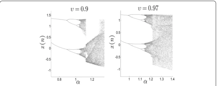
z(0) = 0. The phase portraits are displayed in Figs.2and3for diﬀerent fractional orders. For the numerical simulation, we choose the step sizeα= 0.001. The bifurcation di-agrams are plotted in Fig. 4for diﬀerent values of fractional orderυ. When υ= 0.97, the bifurcation diagrams show a period-doubling cascade route to chaos in the range

α∈[1.1, 1.4]. As the value ofυ decreases, the bifurcation diagram of the fractional or-der map (11) expands along theαaxis and gradually shift to the left.

In addition to visualizing the eﬀect of parameter α on the dynamics of the map, we have seen that the value of the fractional orderυ has an impact on the dynamics. This has been further investigated by plotting the bifurcation of the fractional Stefanski map (11) takingυas the critical parameter. The resulting bifurcation diagram when (α,β) = (1.4, 0.2) and (x(0),y(0)z(0)) = (0, 0, 0) is depicted in Fig.5. We see that chaos is apparent for the intervalυ∈[0.915, 1]. As soon asυdrops below 0.915, the states diverge towards inﬁnity.

(6)

Figure 3Phase space of the fractional-order Stefanski map forυ= 0.969

Figure 4Bifurcation diagrams corresponding to the fractional Stefanski map withαas the critical parameter,

β= 0.2, and diﬀerent fractional ordersυ

(7)

Figure 5Bifurcation diagram of the fractional Stefanski map withυ∈[0, 1] as the critical parameter, (α,β) = (1.4, 0.2) and (x(0),y(0)z(0)) = (0, 0, 0)

Figure 6Estimated Lyapunov exponents of the fractional Stefanski map for (α,β) = (1.4, 0.2), (x(0),y(0)z(0)) = (0, 0, 0), and diﬀerent fractional orders

3.2 Control laws

(8)

Theorem 3 The3D fractional-order Stefanski map(11)is stable under the2D control law results in the modiﬁed system

⎧

Substituting the control law (15) yields the new dynamics

⎧

which can be described more compactly as

Cυ

We aim to show that the zero solution of (18) is globally asymptotically stable, which guar-antees that all states converge towards zero at inﬁnite time. In order to do so, we make use of the stability theory of linear fractional-order maps as described in Theorem2. Simply, we can show that the eigenvalues of the matrix M areλ1=λ3= –1 andλ2=β– 1. It is easy

to see that all the eigenvalues of the matrix M satisfy

|argλi|=π>

(9)

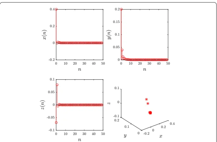
Figure 7The time evolution of the controlled states for the fractional Stefanski map

In order to verify the result of Theorem3, we implemented it numerically in Matlab. The discrete-time states are shown in Fig.7. Clearly, the system is asymptotically stable

and its states converge towards zero.

4 Fractional-order discrete-time Rössler system 4.1 System model and dynamics

The second map we are going to consider here is the 3D Rössler map introduced in [11]

and given by

⎧ ⎪ ⎪ ⎨ ⎪ ⎪ ⎩

x(n+ 1) =b1x(n)(1 –x(n)) –b2(z(n) +b3)(1 – 2y(n)),

y(n+ 1) =b4y(n)(1 –y(n)) +b5z(n),

z(n+ 1) =b6(1 –b7x(n))[(z(n) +b3)(1 – 2y(n)) – 1],

(20)

with states x(n), y(n), andz(n), and parametersb1= 3.8,b2= 0.05,b3= 0.35,b4= 3.78,

b5= 0.2, b6= 0.1, and b7 = 1.9. The Rössler map is well known and has been

exam-ined and applied in countless studies found in the literature. The phase-space portraits

of the Rössler map for initial conditions (x(0),y(0),z(0)) = (0.1, 0.2, –0.5) are displayed in Fig.8.

The fractional-order map corresponding to (20) may be obtained in a similar manner to

(10)

Figure 8Phase space portraits of the standard Rössler map forb1= 3.8,b2= 0.05,b3= 0.35,b4= 3.78,

(11)

Figure 9Phase portraits of the fractional order Rössler map forυ= 0.97

Figure 10 Phase portraits of the fractional order Rössler map forυ= 0.91

0.903. Figure11shows the bifurcation diagram forυ= 0.97 withb1 as the critical

pa-rameter and (b2,b3,b4,b5,b6,b7) = (0.05, 0.35, 3.78, 0.2, 0.1, 1.9). The critical parameter was

varied with the step sizeb1= 0.001. Figure12shows the bifurcation diagram of the

fractional Rössler map with υ∈[0.9, 1] as the critical parameter, (b2,b3,b4,b5,b6,b7) =

(12)

Figure 11 Bifurcation diagram of Rössler system withaas the critical parameter andυ= 0.97

Figure 12 Bifurcation diagram of the fractional Rössler map withυ∈[0, 1] as the critical parameter, (b2,b3,b4,b5,b6,b7) = (0.05, 0.35, 3.78, 0.2, 0.1, 1.9) and (x(0),y(0),z(0)) = (0.1, 0.2, –0.5)

observed forυ>υ0≈0.933. Belowυ0, the map becomes unstable and the states diverge

towards inﬁnity.

Using the same parameters and initial conditions, Fig.13shows the estimated Lyapunov exponents using the Jacobian matrix. Forυ= 1, we observe thatλ1≈λ2> 0, indicating a

hyperchaotic nature of the fractional Rössler map. Similar to Stefanski map, asυreduces, so do the Lyapunov exponents.

In much the same way followed in the previous section, let us now propose adaptive laws to control the fractional Rössler map (21) and drive all of its states towards zero asymp-totically.

Theorem 4 The fractional-order Rössler map becomes asymptotically stable subject to the control laws

⎧ ⎪ ⎪ ⎪ ⎪ ⎪ ⎨ ⎪ ⎪ ⎪ ⎪ ⎪ ⎩

ux(t) = –b1x(t) +b1x2(t) – 2b2z(t)y(t) +b2b3,

uy(t) = –b4y(t) +b4y2(t),

uz(t) = 2b6b3y(t) + 2b6z(t)y(t) +b6(1 –b3) +b6b7x(t)z(t)

– 2b6b7x(t)y(t)z(t) – 2b3b6b7x(t)y(t).

(13)

Figure 13 Estimated Lyapunov exponents of the fractional Rössler map for with

(b2,b3,b4,b5,b6,b7) = (0.05, 0.35, 3.78, 0.2, 0.1, 1.9), (x(0),y(0),z(0)) = (0.1, 0.2, –0.5), and diﬀerent fractional ordersυ

Proof The controlled system corresponding to (21) is of the form

⎧

Substituting the control parameters stated in (23) yields the system dynamics

(14)

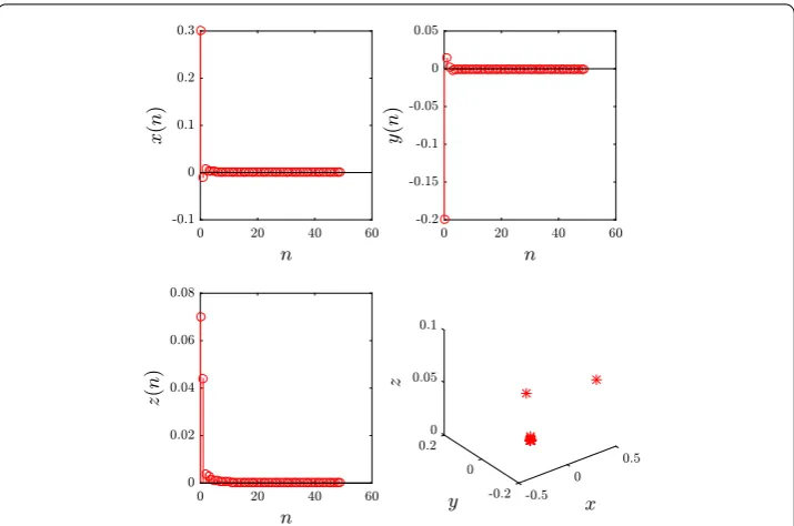
Figure 14 The time evolution of the controlled states for the fractional Rössler map

It is easy to see that the eigenvalues of M satisfy stability condition (8). By means of The-orem2, we know that the zero solution is asymptotically stable and thus the system is

stabilized.

Theorem4was put to the test using the same parameters and initial conditions stated at the beginning of this section and the control laws (23). Figure14shows the time evo-lution of the states, which clearly converge towards zero indicating successful stabiliza-tion.

5 Fractional-order Wang map 5.1 System model and dynamics

Another 3D chaotic map that has an interesting attractor is the hyperchaotic Wang map proposed in [12] and given by

⎧ ⎪ ⎪ ⎨ ⎪ ⎪ ⎩

x(n+ 1) =a3y(n) + (a4+ 1)x(n),

y(n+ 1) =a1x(n) +y(n) +a2z(n),

z(n+ 1) = (a7+ 1)z(n) +a6y(n)z(n) +a5.

(27)

Figure15shows the phase portraits for the following set of parameters:

(a1,a2,a3,a4,a5,a6,a7) = (–1.9, 0.2, 0.5, –2.3, 2, –0.6, –1.9).

(15)

Figure 15 Phase portraits of the standard discrete-time Wang system

We follow the same lines of the previous two sections to arrive at the fractional-order discrete-time Wang map given by

⎧ ⎪ ⎪ ⎨ ⎪ ⎪ ⎩

Cυ

ax(t) =a3y(t– 1 +υ) +a4x(t– 1 +υ),

Cυ

ay(t) =a1x(t– 1 +υ) +a2z(t– 1 +υ),

Cυ

az(t) =a7z(t– 1 +υ) +a6y(t– 1 +υ)z(t– 1 +υ) +a5.

(28)

The numerical formulas can be obtained in a similar fashion to the previous two sec-tions by means of Theorem1. It can be easily shown that the fractional Wang map (28) is chaotic. Consider the casea= 0 and initial conditions (x(0),y(0),z(0)) = (0.05, 0.03, 0.02). Figures16and17show the resulting attractors for the fractional orders υ= 0.97 and

υ = 0.969, respectively. We have also plotted the bifurcation diagram with the critical parametera3 being varied at steps ofa.3 = 0.001 and the remaining parameters

cho-sen as (a1,a2,a4,a5,a6,a7) = (–1.9, 0.2, –2.3, 2, –0.6, –1.9). The bifurcation duration was

set ton= 200. The bifurcation diagrams are depicted in Fig.18for diﬀerent fractional ordersυ. In Fig.19, we show the bifurcation diagram of the fractional Wang map (28) with υ ∈[0.9, 1] as the critical parameter. We see that the map exhibits a chaotic be-havior over a short interval of fractional orders. Chaos clearly disappears completely for

υ<υ0≈0.915. In fact, whenυ< 0.968, the chaotic behavior is intermittent and has a very

short range.

The Lyapunov exponents of the fractional Wang map (28) with the same previous pa-rameters and initial conditions are depicted in Fig.20. Forυ= 1, we see thatλ1>λ2> 0,

(16)

Figure 16 Phase space portraits of the fractional-order Wang map forυ= 0.97

Figure 17 Phase space portraits of the fractional-order Wang map forυ= 0.969

(17)

Figure 18 Bifurcation diagrams of the fractional-order Wang map for diﬀerent fractional orders

Figure 19 Bifurcation diagram of the fractional Rössler map withυ∈[0, 1] as the critical parameter, (a1,a2,a4,a5,a6,a7) = (–1.9, 0.2, –2.3, 2, –0.6, –1.9) and (x(0),y(0),z(0)) = (0.05, 0.03, 0.02)

Theorem 5 The fractional-order Wang map(28)is stabilized subject to the control laws

⎧ ⎪ ⎪ ⎨ ⎪ ⎪ ⎩

ux(t) = 2x(t),

uy(t) = –a1x(t) –y(t),

uz(t) =z(t) –a6y(t)z(t) –a5.

(29)

Figure21depicts the time evolution of the states for the controlled fractional-order discrete-time Wang system. The states are observed to converge towards zero asymptot-ically, indicating that the system is stabilized.

6 A combined synchronization scheme

(18)

Figure 20 Estimated Lyapunov exponents of the fractional Wang map for with

(a1,a2,a4,a5,a6,a7) = (–1.9, 0.2, –2.3, 2, –0.6, –1.9), (x(0),y(0),z(0)) = (0.05, 0.03, 0.02), and diﬀerent fractional ordersυ

(19)

communications and data encryption as shown in [37], for instance. The application of this type of systems is mainly dependent on our ability to synchronize two systems start-ing from diﬀerent initial conditions such that they end up followstart-ing the same trajectory asymptotically. In this section, we propose a combined synchronization scheme for the three fractional maps discussed herein. We consider as our drive system the fractional Rössler map given fort∈Na+1–υby

As for the response system, we consider a combination of the fractional Stefanski map described by

and the fractional Wang map given by

⎧

The drive system (30) and the response systems (31)–(32) are said to be combination-synchronized if there exist controllersu1(t), . . . ,u6(t) such that the synchronization errors

(20)

witht∈Na+1–υ, converge to zero asymptotically, i.e.,

lim

t→∞ei(t)= 0, i= 1, 2, 3. (35)

The following theorem proposes suitable adaptive laws for controllersu1(t), . . . ,u6(t) in

order to guarantee that (35) holds.

Theorem 6 Subject to

the drive system(30)and the response systems(31)–(32)are combination-synchronized.

Proof Taking the fractional diﬀerences of the synchronization errors (34) and substituting the proposed controllers (36) yields the error dynamics

Cυ

In order to ensure that the drive and response systems are synchronized, we must establish that the errors in (37) converge towards zero asymptotically. It is easy to see that the matrix Msatisﬁes stability condition (8) of Theorem2. Hence, we ﬁnd that the zero solution of the error system (37) is asymptotically stable and, consequently, the drive system (30) and response systems (31)–(32) are combination-synchronized.

Using the parameters speciﬁed in (33) witha= 0 and the same initial conditions from previous sections, a Matlab program was implemented to track the time evolution of the errors (34) and ensure they converge to zero asymptotically. The results are depicted in Fig.22. It is obvious that the combination-synchronization is successful. The errors clearly decay to zero and the sums of the slave states match those of the master.

7 Concluding remarks and future work

(21)

Figure 22 Time evolution of the synchronization errors for the proposed combined synchronization scheme

demonstrated by the phase portraits, as well as the bifurcation analysis and the estima-tion of Lyapunov exponents. The dynamics of these maps were analyzed by means of numerical methods. In addition, we presented three distinct stabilization laws for the proposed maps, whereby adaptive additive terms are included in the maps to drive their states towards zero asymptotically. The stability and convergence of these schemes was established by means of the stability theory of linear fractional discrete systems. Fur-thermore, we proposed a combination-synchronization scheme considering the fractional Rössler map as a drive system and a combination of the fractional Stefanski and Wang maps as the response system. The convergence of the stabilized states as well as the syn-chronization errors towards zero was illustrated by means of numerical simulation re-sults.

(22)

Acknowledgements

The authors acknowledge Prof. GuanRong Chen, Department of Electronic Engineering, City University of Hong Kong for suggesting many helpful references.

Funding

Xiong Wang was supported by the National Natural Science Foundation of China (No. 61601306) and Shenzhen Overseas High Level Talent Peacock Project Fund (No. 20150215145C).

Availability of data and materials

Not applicable.

Competing interests

The authors declare that they have no competing interests.

Authors’ contributions

AAK, AO and SB suggested the model, helped in results’ interpretation and manuscript evaluation. GG and XW and VTP helped to evaluate, revise and edit the manuscript. GG, XW and FEA supervised the development of the work. VTP and FEA drafted the article. All authors read and approved the ﬁnal manuscript.

Author details

1_{Laboratory of Dynamical System and Control, University of Larbi Ben M’hidi, Oum El Bouaghi, Algeria.}2_{Department of}

Mathematics and Computer Science, University of Larbi Tebessi, Tebessa, Algeria.3_{Electrical Engineering Department,}

College of Engineering at Yanbu, Taibah University, Medina, Saudi Arabia.4_{Dipartimento Ingegneria Innovazione,}

Universita del Salento, Lecce, Italy.5_{Institute for Advanced Study, Shenzhen University, Shenzhen, P.R. China.}6_Nonlinear

Systems and Applications, Faculty of Electrical and Electronics Engineering, Ton Duc Thang University, Ho Chi Minh City, Vietnam.7_{Department of Information Technology, Faculty of Computing and IT, King Abdulaziz University, Jeddah, Saudi}

Arabia.

Publisher’s Note

Springer Nature remains neutral with regard to jurisdictional claims in published maps and institutional aﬃliations. Received: 18 October 2018 Accepted: 16 September 2019

References

1. Lian, K.Y., Chiang, T.S., Liu, P.: Discrete-time chaotic systems: applications in secure communications. Int. J. Bifurc. Chaos10, 2193 (2000)

2. Feki, M., Robert, B., Gelle, G., Colas, M.: Secure digital communication using discrete-time chaos synchronization. Chaos Solitons Fractals18, 881–890 (2003)

3. Guo, L.J., Geng, X.Y.: Chaos communication based on synchronization of discrete-time chaotic systems. Chin. Phys. 14, 274 (2005)

4. Stork, M.: Digital chaotic systems examples and application for data transmission. In: Proc. Int. Conf. Electrical & Electronics Eng. (ELECO’2009), Bursa, Turkey, pp. 78–82 (2009)

5. Kocarev, L., Szczepanski, J., Amigo, J.M., Tomovski, I.: Discrete chaos–I: theory. IEEE Trans. Circuits Syst. I, Regul. Pap.53, 1300–1309 (2006)

6. Hénon, M.: A two-dimensional mapping with a strange attractor. Commun. Math. Phys.50, 69–77 (1976) 7. Lozi, R.: Un atracteur étrange du type attracteur de hénon. J. Phys.39, 9–10 (1978)

8. Hitzl, D., Zele, F.: An exploration of the Hénon quadratic map. Phys. D, Nonlinear Phenom.14, 305–326 (1985) 9. Baier, G., Sahle, S.: Design of hyperchaotic ﬂows. Phys. Rev. E51, 2712–2714 (1995)

10. Stefanski, K.: Modelling chaos and hyperchaos with 3D maps. Chaos Solitons Fractals9, 83–93 (1998)

11. Itoh, M., Yang, T., Chua, L.: Conditions for impulsive synchronization of chaotic and hyperchaotic systems. Int. J. Bifurc. Chaos11, 551–558 (2001)

12. Wang, X.Y.: Chaos in Complex Nonlinear Systems. Publishing House of Electronics Industry, Beijing (2003)

13. Atici, F.M., Eloe, P.W.: Discrete fractional calculus with the nabla operator. Electron. J. Qual. Theory Diﬀer. Equ. Spec. Ed. I2009, 3, 1–12 (2009)

14. Abdeljawad, T.: On Riemann and Caputo fractional differences. Comput. Math. Appl.62, 1602–1611 (2011) 15. Abdeljawad, T., Baleanu, D., Jarad, F., Agarwal, R.P.: Fractional sums and differences with binomial coefficients. Discrete

Dyn. Nat. Soc.2013, 104173 (2013)

16. Goodrich, C., Peterson, A.C.: Discrete Fractional Calculus. Springer, German (2015)

17. Baleanu, D., Wu, G., Bai, Y., Chen, F.: Stability analysis of Caputo-like discrete fractional systems. Commun. Nonlinear Sci. Numer. Simul.48, 520–530 (2017)

18. Wu, G., Baleanu, D.: Discrete fractional logistic map and its chaos. Nonlinear Dyn.75, 283–287 (2013) 19. Hu, T.: Discrete chaos in fractional Hénon map. Appl. Math.5, 2243–2248 (2014)

20. Shukla, M.K., Sharma, B.B.: Investigation of chaos in fractional order generalized hyperchaotic Hénon map. Int. J. Electron. Commer.78, 265–273 (2017)

21. Wu, G.C., Baleanu, D.: Discrete chaos in fractional delayed logistic maps. Nonlinear Dyn.80, 1697–1703 (2015) 22. Boccaletti, S., Grebogi, C., Lai, Y.C., Mancini, H., Maza, D.: The control of chaos: theory and applications. Phys. Rep.329,

103–197 (2000)

23. Fradkov, A.L., Evans, R.J., Andrievsky, B.R.: Control of chaos: methods and applications in mechanics. Philos. Trans. R. Soc. A, Math. Phys. Eng. Sci.364, 2279–2307 (2006)

(23)

25. Ouannas, A., Azar, A.T., Abu-Saris, R.: A new type of hybrid synchronization between arbitrary hyperchaotic maps. Int. J. Mach. Learn. Cybern.8, 1887–1894 (2017)

26. Ouannas, A., Grassi, G.: A new approach to study co-existence of some synchronization types between chaotic maps with diﬀerent dimensions. Nonlinear Dyn.86, 1319–1328 (2016)

27. Ouannas, A., Odibat, Z.: Generalized synchronization of diﬀerent dimensional chaotic dynamical systems in discrete-time. Nonlinear Dyn.81, 765–771 (2015)

28. Ouannas, A.: A new generalized-type of synchronization for discrete chaotic dynamical system. J. Comput. Nonlinear Dyn.10, 061019 (2015)

29. Grassi, G., Ouannas, A., Pham, V.T.: A general uniﬁed approach to chaos synchronization in continuous-time systems (with or without equilibrium points) as well as in discrete-time systems. Arch. Control Sci.28, 135–154 (2018) 30. Wu, G., Baleanu, D.: Chaos synchronization of the discrete fractional logistic map. Signal Process.102, 96–99 (2014) 31. Wu, G., Baleanu, D., Xie, H., Chen, F.: Chaos synchronization of fractional chaotic maps based on the stability

condition. Physica A460, 374–383 (2016)

32. Liu, Y.: Chaotic synchronization between linearly coupled discrete fractional Hénon maps. Indian J. Phys.90, 313–317 (2016)

33. Megherbi, O., Hamiche, H., Djennoune, S., Bettayeb, M.: A new contribution for the impulsive synchronization of fractional–order discrete–time chaotic systems. Nonlinear Dyn.90, 1519–1533 (2017)

34. Huang, L.L., Baleanu, D., Wu, G.C., Zeng, S.D.: A new application of the fractional logistic map. Rom. J. Phys.61, 1172–1179 (2016)

35. Cermak, J., Gyori, I., Nechvatal, L.: On explicit stability condition for a linear fractional diﬀerence system. Fract. Calc. Appl. Anal.18, 651–672 (2015)

36. Wu, G.C., Baleanu, D.: Jacobian matrix algorithm for Lyapunov exponents of the discrete fractional maps. Commun. Nonlinear Sci. Numer. Simul.22, 95–100 (2015)