R E S E A R C H
Open Access
Forecasting the next handoff for users moving
with the Random Waypoint mobility model
Enrica Zola
*, Francisco Barcelo-Arroyo and Israel Martín-Escalona
Abstract
Users in a cellular network can move while their connections are handed off to different access points. Studies prove that the mobility pattern followed have a strong impact on performance metrics (i.e., handoff (HO) rate, cell residence time). Recently, some key aspects of the Random Waypoint mobility model have been studied in depth, but relating those studies with different cellular layouts has not been reported. Interest in forecasting the cell to which a device may be handed off depending on the movement pattern is twofold. First, it gives insight into properties and statistics of the mobility model. Second, and from a more practical perspective, it is useful to manage resource allocation and reservation strategies in order to smooth the HO process. The goal of this article is to provide an analytical framework for these predictions in a simple layout. Given a node’s current location and the timestamp and location of the last waypoint, an approximation for HO during timeΔtis derived. The analysis is provided along with numerical examples and simulations for a symmetrical layout and uniform speed distribution. Results shed light on how useful more advanced strategies can be.
Keywords:Handoff probability forecast, Random Waypoint mobility model, Analytical framework
1. Introduction
Users in a cellular network move while their connections are transferred between access points. This process is known as handoff (HO). This same concept holds for different technologies (e.g., GSM, UMTS, LTE, WiFi, ZigBee, WiMAX), although the name of the key element changes according to the specific standard (e.g., base station—BS, node B, access point—AP). As the user moves, the quality of the signal received from the current cell may decrease under some acceptable threshold. This event will trigger the HO procedure [1]. The time needed to transfer the ongoing communications to the new cell is crucial [2,3] since if this process lasts too long the user may suffer degradation in the quality of the ongoing services. In some cases, it may lead to a drop in the communication [4]. This issue is particularly important for delay-sensitive applications such as video and audio streaming.
Mobility prediction techniques allow the network to prepare for the HO in advance (e.g., booking resources for the expected HO in the destination cell) [5]. Re-source demands could fluctuate abruptly due to the
movement of high data rate users. If one can predict requests of bandwidth at a cell, the overall network performance would improve. The goal of our research is to provide a mathematical framework through which the percentage of HO for users moving with a known mobility pattern can be forecasted. By properly handling this information at the BSs, the network can better manage the resources and prepare the HOs, hence redu-cing the time needed to authenticate in the connection in the new cell and decreasing the probability of drop-ping the connection. However, how this prediction is used by the network is out of the scope of this article.
Structural approaches study mobility through math-ematical models that try to represent human or vehicle mobility. Mobility models play a key role when planning a wireless network (i.e., resource allocation, location up-dating, and channel holding time). The Random Waypoint (RWP) mobility model [6] is simple and has extensively been used in simulation studies. Kurkowski et al. [7] ana-lyze MANET simulation studies published in a premiere conference for the MANET community between 2000 and 2005. They found that 66% of the studies involving mobil-ity used the RWP mobilmobil-ity model. Despite it has been criticized for not being representative of how humans * Correspondence:[email protected]
Telematics Engineering Department, Universitat Politècnica de Catalunya (UPC), Barcelona, Spain
actually move, it is still largely used in many studies [8-13]. Rojas et al. [14] validate the RWP against real mobility data. With small changes to the distributions used in the RWP (e.g., non-uniform distribution of the waypoints), the authors show that it can be used as a good model for mobility in large geographic areas such as a city. Con-sidering that extracting a mobility pattern from real traces is complex and, anyway, it would be specific to the envir-onment and conditions from which it has been extracted, the use of the RWP in simulation studies is widely ac-cepted. Many researchers have studied the impact of the RWP on routing protocols [15,16], connectivity probabil-ities [17,18], cell residence time [19-21], and cell change rate [20,22]. However, prediction of the probability of HO to a given cell for users moving according to the RWP mobility pattern has not yet been addressed.
In this article, a detailed description of the analytical framework to forecast the next cell to which a user HOs within a certain period of time is provided. The frame-work was partially presented in [23]. This analysis follows previous research on statistical characteristics of the RWP mobility model (i.e., length and duration of the straight movement between two waypoints [22], node distribution [24,25]). Moreover, simulation results are shown in this study in order to validate the analyt-ical model and check the small impact of the necessary simplifications done. The importance of this study is twofold. First, it provides a deeper insight into the statistics of the RWP mobility model, extending previ-ous analysis [22,24-26]. This statistical knowledge provides a better understanding of the interplay of the mobility pattern with network parameters. Second, and from a more practical perspective, the HO prediction is useful to manage resource allocation and reservation strategies. According to our model, few requirements are needed to perform the forecast of a possible HO in the near future: knowledge of the cells’ locations and geometries; knowledge of user’s position (e.g., through GPS); knowledge of when and where the user changed direction of movement and speed for the last time (e.g., through inertial sensors). Despite the model has been applied to a 4-cell scenario (see Section 4.3), this meth-odology can be generalized to any symmetrical layout in which fixed BSs are located at the vertices of any regular polygon. Researchers can take advantage of the prediction framework presented in this article for their simulations. As an example, it can be applied in studies on allocation strategies for QoS improvement in cellular networks.
The remainder of this article is organized as follows. Section 2 provides a brief overview of the related litera-ture. The RWP mobility model is explained in Section 3. The method proposed to estimate the probability of HO to a given cell is shown in Section 4. The method is then applied to different cases: numerical results are provided
in Section 5, while simulation results in Section 6. Section 7 summarizes the main conclusion.
2. Related work
A lot of research has been conducted to propose schemes that try to decrease the HO latencies. This problem is particularly important in IEEE 802.11 networks where it has been proven that these latencies are especially high [2]. Since the scanning time needed to find a new candi-date AP is the most constraining phase, many proposals can be find which aim to reduce it. Velayos and Karlsson [3] suggest reducing the link-layer detection time to three consecutive lost frames and to use different timers for the active scanning, thus reducing the search time at least by 20%. An HO procedure is presented in [27], which reduces the discovery phase using a selective scanning algorithm and a caching mechanism. Modification in the standard active scan is proposed in [28]; a user should be able to periodically probe in the background for APs on other channels even when it is already associated with an AP. These make-before-brake algorithms lead to a signifi-cant reduction in MAC layer HO overhead. Similarly, in order to limit the frequency of channel scanning, an adap-tive mechanism is recommended in [29] to dynamically adjust the threshold triggering the channel scanning operations. In addition tohorizontal HO, i.e., HO between cells within the domain of a single wireless access technol-ogy, recent interest has been directed towardvertical HO
(VHO), which allows users to HO among heterogeneous wireless access networks [30,31]. Lee et al. [32] investigate the problem of VHO from a 3 G cellular network to a WLAN hotspot. They propose a call admission control that allows the WLAN to limit the VHOs and reduce unnecessary VHO processing. Ben Ali and Pierre [33] evaluate the impact of VHO on the performance of the voice admission control in different mobility environments.
algorithm is designed for eNodeB’s HO preparation, thus improving the HO in 3 G LTE systems.
Prediction of users’ movement is also possible using trace data [36]. For HO success, the most important predictions occur when moving into highly populated cells. Other studies exploit real traces to analyze the predictability of users’ movements inside the network [37,38]. Sricharan and Vaidehi [37] examine real-time mobility traces and identify key mobility parameters. A generic framework for mobility prediction is proposed in [38] where a model is proposed to predict the sequences of a user’s path from observed sequences. Libo et al. [39] conducted an extensive empirical com-parison of four important classes of location predictors in order to prove which could most accurately predict the next cell for a mobile wireless-network user. They found that the complex predictors were at best only negligibly better than the simple Markov predictor.
Much effort has been made to gain understanding of the implications that the use of the RWP model may cause. The“steady-state”problem has been addressed in [22,40]. By giving a formal description of the RWP model in terms of a discrete-time stochastic process, Bettstetter et al. [22] investigate the length and time of the movement between waypoints, the spatial distribu-tion of nodes, the direcdistribu-tion angle at a new waypoint, and the cell change rate. Navidi and Camp [40] derive the stationary distributions for location, speed, and pause time. The spatial node distribution of nodes is also addressed in [24,25]. Given that the RWP tends to bring the nodes to the centre of the area, Bettstetter et al. [24] proposed to initially distribute the nodes according to a given pattern so that the network starts in the steady state. Hyttia et al. [25] propose a general expression for the node distribution without using approximations. An exact formula for the mean arrival rate across an arbitrary curve is presented in [20]. This result, together with the distribution of a node’s loca-tion, allows the computation of other metrics, such as the mean HO rate and the mean dwell time. Pla and Casares-Giner [19] propose a model of the sojourn time in the overlap area for users moving according to the RWP. To simplify their study, they assume that waypoints cannot fall inside the overlap area. The ob-tained results show that the common assumption of exponential distribution for this time is not suitable.
3. Random waypoint mobility model
Modeling the mobility of terminals in wireless networks, where the connection has to be handled through several APs, is a key in order to forecast the quality of service and design the necessary resources. In general, high mobility leads to poorer quality of service since more HO that cause extra overhead are performed. While it is obvious
that faster speeds tend to cause more HO, it must be highlighted that the mobility pattern is also related to the HO rate: a terminal moving in circles close to the AP at high speed may not require HO while another one moving away from the AP will certainly require an HO soon.
The RWP was introduced in [6]. In this model, each node is assigned an initial location (WP0) and a destin-ation (WP1), which are chosen independently and uni-formly within thewhole area(i.e., the area where nodes can move, which is generally assumed to be convex). A speed (v) is assigned as well, which is chosen uniformly or according to any other distribution from an interval (vmin to vmax) and independent of the initial location and destination. Between the two waypoints WP0 and WP1, the node follows a straight line and moves at a constant speed. The movement between two waypoints is referred to as alegortransition. After reaching WP1, a new destination and a new speed are chosen inde-pendent of previous destinations and speeds. The node may remain paused for some randompause timebefore starting its movement toward the next waypoint. For simplicity, pause times are not considered in this study.
Exact formulas for the probability density function (pdf) of the distance between two waypoints, i.e., pdf of the transition length,fL(ℓ) in different scenarios are provided in
[22,25]. According to the geometry and dimensions of the area, the mean distance can be evaluated.
4. Probability of handoff to a given cell 4.1. Problem statement
The objective of the study is to estimate the probability of HO to a given cell before a given period of time (Δt) elapses, provided that we know where and when the last waypoint was reached. The forecast is performed under the following assumptions:
The whole areaAis a circle of radiusR, and APs are placed at the corners of a regular polygon inside the circle. Any regular polygon can be considered (e.g., a square as shown in Section4.3).
Ideal conditions are considered (i.e., noise and fading are not taken into account).
Coverage areas have a circular shape. Current positionPtat timetis known.
Position and time of the last waypoint (WPjat timej)
are known (i.e., where and when the node changed to the present direction and speed). Alternatively, movement direction and time of the last waypoint can be used to derive the position of the last waypoint. It is assumed that the number of waypointsX(Δt) that
a node may reach duringΔtis smaller or equal to one. In general, the node may perform multiple HOs in
When the node is inside the coverage areas of two or more APs (i.e., overlapping area), the HO starts when the node exits the coverage area of the AP to which it is currently associated. Other HO strategies may be applied, with minor changes in the proposed framework.
The following parameters are considered (a layout with four APs is depicted in Figure 1 for better understanding):
γjrepresents the current angle of direction andvj
the current speed.
Yis the distance between WPjandPt(i.e., distance already traveled at speedvjin directionγj).
xt,xA, andxtAPrepresent the distances fromPtto the cell boundaries, the boundaries ofAand the borders of the neighboring cell in directionγj, respectively
(see Figures1and2). Theneighboring cellis the cell toward which the MN is moving in directionγj. If there are two intersections with the
neighboring cell, they are identified with xtAP+ and xtAP– (see Figure 2b).
The definition of a node’s movement directionγjin a
two-dimensional space can be better understood through Figure 1. As shown in [22], the outcome of this angle depends on both polar coordinates of Pt(e.g., dt
andΦt). Thus, a second alternative direction angleθtis
introduced. This angle is defined in a way thatθt= 0 for
movements going through the center of the circular area. A major advantage of this definition is that the outcome of θt is independent of the polar angle Φt. It
can directly be mapped onto γj for a given Φt. If we
define that counterclockwise angles count positive
γj¼θtþφtþπ: ð1Þ
Figure 1Layout with four APs.Current cell is cell 2 (AP2). The distance to the cell boundary (xt) in current directionγjis displayed,
together with other parameters used in the analysis.
Figure 2Layout with four APs.The distances from the whole area (xA) and neighbouring cell (xtAP) in current directionγjare displayed in
In a circular layout, the formula for the maximum length of the movement from Ptin direction γj (i.e.,xA
according to previous definition) is [22]
xAð Þ ¼θt dt:cosθtþ
ffiffiffiffiffiffiffiffiffiffiffiffiffiffiffiffiffiffiffiffiffiffiffiffiffiffiffiffiffiffiffiffiffi
R2 d
t:sinθt
ð Þ2
q
; ð2Þ
where dt and Φt are the polar coordinates of current
positionPtwith respect to the center ofA. Similarly
xt θ0t ¼d
0
t:cosθ
0
tþ
ffiffiffiffiffiffiffiffiffiffiffiffiffiffiffiffiffiffiffiffiffiffiffiffiffiffiffiffiffiffiffiffiffiffiffi r2
cell d
0
t:sinθ
0
t
2
q
; ð3Þ
xtAPþ θt ¼dt:cosθ
t þ
ffiffiffiffiffiffiffiffiffiffiffiffiffiffiffiffiffiffiffiffiffiffiffiffiffiffiffiffiffiffiffiffiffiffiffiffi r2
cell dt:sinθt
2
q
xtAP θt ¼dt:cosθ
t
ffiffiffiffiffiffiffiffiffiffiffiffiffiffiffiffiffiffiffiffiffiffiffiffiffiffiffiffiffiffiffiffiffiffiffiffi r2
cell dt:sinθ
t
2
q ;
8 < :
ð4Þ
whered’tis the distance ofPtto the center of the current
cell, θ’t=γj –αt –π (see Figure 1),αtis the angle of Pt
with respect to the center of the cell,rcell is the radius of the cell, d*t is the distance of Pt to the center of the
neighboring cell (i.e., cell 1 in Figure 2), θ*t=γj– α*t –π,
andα*tis the angle ofPtwith respect to the center of the
neighboring cell. From (1), we can write
θ0
t ¼θtþφtαt; ð5Þ
θ
t ¼θtþφtα
t: ð6Þ
4.2. Probability of handoff
Given the number of waypoints X(Δt) that a node may reach duringΔt, the probability of HO can be written as
Pr HO inf Δtg ¼X 1
i¼0
PrfHO inΔtjXð Þ ¼Δt ig:
PrfXð Þ ¼Δt ig: ð7Þ
According to initial assumptions, Pr{X(Δt) =i} is zero fori> 1. Thus, Equation (7) can be written as
Pr HO inf Δtg ¼PrfHO inΔtjXð Þ ¼Δt 1g:PrfXð Þ ¼Δt 1g þPrfHO inΔtjXð Þ ¼Δt 0g:PrfXð Þ ¼Δt 0g ¼Pr HOaf g:PrfXð Þ ¼Δt 1g
þPr HObf g:ð1PrfXð Þ ¼Δt 1gÞ; ð8Þ
where Pr{X(Δt) = 1} represents the probability of reaching the waypoint duringΔt, Pr{HOa}is the probability of HO given that a waypoint is reached duringΔt, while Pr{HOb} is the probability of HO given that node moves on same direction and at same speed during Δt. Because the current direction of movement γjand the current speed vjare known, Pr{HOb} only depends on the distance to
the cell border in directionγjand can easily be calculated.
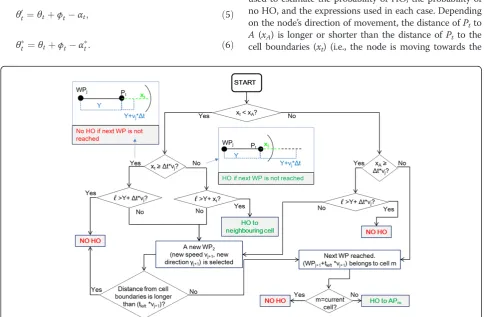
The flow charts in Figures 3 and 4 show the algorithm used to estimate the probability of HO, the probability of no HO, and the expressions used in each case. Depending on the node’s direction of movement, the distance ofPtto A(xA) is longer or shorter than the distance ofPtto the
cell boundaries (xt) (i.e., the node is moving towards the
center ofAor in opposite direction, respectively). Figure 3 shows that, in the first case (xt<xA), an HO is
performed if the distance to the cell boundaries is shorter than the distance walked at given speed during Δt(xt<vj. . .Δt) and the distance between two waypoints
(ℓ) is longer than Y+xt (i.e., the node does not reach
the waypoint before exiting its current cell, thus Pr {HOb} is one). On the other hand, if xt≥xA, then an
HO is performed only if the distance to the boundaries ofA is shorter than the distance walked at given speed during Δt (xA< vj. . .Δt) and the point reached in the
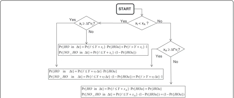
new direction falls outside the current cell. In all the other cases, the node will remain inside its current cell. In Figure 4, the corresponding expressions for each case are provided.
In the following sections, expressions for the prob-ability of reaching the next waypoint and for Pr{HOa} are provided.
4.2.1. Probability of reaching the next waypoint duringΔt
Recall that the node is located at Pt at time t and
that it has been traveling a distance Yfrom previous waypoint WPj. The next waypoint may be located at
any point on the straight line between Pt and Pt+vj
⋅Δt (if xt≥vj⋅Δt and xt< xA), between Pt and Pt+xt
(if xt<vj⋅Δt and xt< xA), or between Pt and Pt+xA
(if xt≥xA). We define this generic point on the
current direction of movement at generic distance r
from Pt asS(r) (i.e., S(r = 0)≡Pt). The expression Pr{X
(t+r/vj) = 1} represents the probability of reaching the
next waypoint after traveling a distancerat current speed
vj, where tþvrj≤Δt. This probability can be rewritten as
the probability that the distance between two waypoints (ℓ) is shorter than a generic distanceL = Y + r. Thus, de-pending on the geometry and on the current speed, we find different expressions
Figure 4Formulas used to determine the probability of HO and no HO.
Prfreach the next waypoint duringΔtg ¼
where fL(ℓ|θt) is the pdf of the distance between two
waypoints provided that the current direction of move-ment is known. According to [22], ifAis a circle of radius
R;fLðljθtÞ ¼πR8 :2⋅lR arccos 2⋅lR 2l⋅R:
ffiffiffiffiffiffiffiffiffiffiffiffiffiffiffiffiffiffiffiffi 1 l
2⋅R
2
q
.
4.2.2. Probability of HO when the waypoint is reached (Pr{HOa})
Consider that the node reaches the next waypoint at the
generic point S(r) at time tþvrj
. We can define tr as
the remaining time beforeΔtelapses. It can take values between (0,Δt). We can write
tr¼Δt
r vj:
ð10Þ
The probability that the node reaches another way-point during tr is small when Δt is small. According to
our initial assumption, by accurately choosing Δt, we can discard the possibility that another waypoint is reached, which would highly complicate the solution. The polar coordinates of the waypoint are (dWP, ΦWP). At this point, a new waypoint will randomly be selected insideAand the node will start moving in a new direc-tion. According to Bettstetter et al. [22], nodes take a non-uniformly distributed angle of direction at each new
waypoint. The pdf of this angle depends on the shape of
Aand the starting waypoint of the node. Thus, in a circu-lar area of radiusR, the pdf of the angle of directionγis
fΓðγjðdWP;φWPÞÞ ¼fΘðθjdWPÞ ¼
1 2πR2 x
2
Að Þθt : ð11Þ
Moreover, a new speed will randomly be selected at the waypoint. The points reached after tr at maximum
and minimum speed are estimated in each possible dir-ection of movement. These points identify a crown where the node may be located afterΔt. Since the speed is uniformly distributed between vmin and vmax, each point among (vmin⋅tr) and (vmax⋅tr) is equally probable.
Each direction may be selected according to (11). The area where the node may move can be divided into two areas: one inside the current cell (i.e., no HO is performed) and another one inside one (at least) of the neighboring cells (i.e., an HO is performed). According to previous definitions, the latter is Pr{HOa|r}. As S(r) moves away from Pt, the radius of the crown will
de-crease and the distances and angles will change. Thus, we have to evaluate Pr{HOa|r} at any distancerfromPt.
The final expression to estimate the probability of HO given that the waypoint is reached duringΔtis
where Pr{HOa|r} represents the probability of HO given that the next waypoint isS(r), andfR(r) is the pdf of the
possible positions S(r). Note that the waypoints are uni-formly selected inA.
4.3. Application to four APs
In order to illustrate how the analytical framework provides the forecast of the HO in a specific scenario, we will consider a layout with four APs. The coverage area of each AP is a circular area of radius rcell. The APs are located at the vertices of a square whose side is
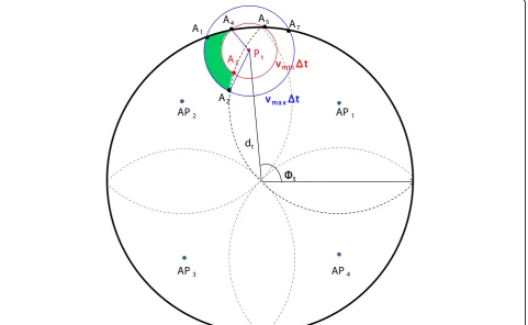
R, as shown in Figure 1. In Figure 5, the method to
calculate the probability of HO when the next waypoint is Pt(i.e., Pr{HOa|r= 0}) is illustrated. From the current
point Pt, a circular crown can be drawn with inner
ra-dius (vmin⋅Δt) and outer radius (vmax⋅Δt). The crown represents the area where the node may be located if it changes its direction of movement and speed atPt.
Be-cause the speed distribution is uniform between vmin and vmax, the distribution of the node locations’ inside this area is uniform too. Points inside the crown but out-side A are discarded (i.e., they fall outside the area of movement). Angles for the points A1, A4, A5, and A7 should be estimated; we refer to these angles asθA1,θA4,
Figure 6Distances used to evaluate Pr{HOa}.
Pr HOf ag ¼ Zvj:Δt
0
Pr HOa ro:fRð Þdrr ifxt θ
0
t ≥vj:Δtandxt θ
0
t <xAð Þθt
n
Z
xt θ
0
t
0
Pr HOa r o
⋅fRð Þdrr if xt θ
0
t <vj⋅Δtandxt θ
0
t <xAð Þθt
n
Z
xAð Þθt
0
Pr HOa r o
⋅fRð Þdrr ifxt θ
0
t ≥xAð Þθt ; ð12Þ
n 8
θA5, andθA7, respectively. The HO area is represented in
green in Figure 5 (i.e., the node is currently associated with AP1). It spans from angle θA4 and θA2. The
prob-ability of HO in this case equals the probprob-ability of HO to AP2 and can be evaluated as
Pr HOa rf j ¼0g
¼
ZθA2
θA4
fΘðθjdtð ÞrÞ:
minðd1ð Þr;d2ðθ;rÞ;d3ðθ;rÞÞ minðd1ð Þr;d3ðθ;rÞÞ ;
ð13Þ
whereris the distance already walked fromPt(i.e., zero
in this case), d1(r) is the difference of the two radii of the crown (see Figure 6), d2(θ,r) is the difference be-tween the outer radius of the crown andxt(θ’t,r),d3(θ,r)
is the difference of xA(θt,r) and the inner radius of the
crown, andθrepresents all possible angles of movement from the current position with respect to the centre of
A.fΘ(θ|dt(r)) is defined in (11) and represents the pdf of
the direction angle θprovided that we are at distancedt
(r) from the centre ofA.
The integral in (13) cannot be evaluated because the integrand function changes in the interval of integration. Instead, a sum of integrals is used where the minimum function is substituted by the corresponding minimum distance at each interval (see Section 5). Expressions for
d1(r), d2(θ,r), and d3(θ,r) are provided in Appendix 1. Depending on the current position of the node, the cir-cular crown intersects the cell boundaries and/or A at different points. All of the other possible distances (d4(θ, r),d5(θ,r),d6(θ,r)) are provided in Appendix 1. Refer to Figure 6 to better understand these values.
Equation 13) is evaluated iteratively at any point S(r) according to (12). In each iteration, the time decreases as the node moves at speed vjin direction γj; then, the
radius of the crown will decrease, and the distances and
Figure 8Example of calculation of Pr{HOa} with an
approximation in the estimation of Pr{HOAP3} and Pr{HOAP4} (i.e., 0.5⋅d1is used instead of the exact distances displayed in yellow and orange in the zoom).
WPj
AP3 AP4
AP1 AP2
x xt(θt(r),r)
xA(θt(r), r)
ϕt(r)
R/2
0
R/2 -R/2
-R/2
0
xtAP+(θt*(r),r) R
-R R
Pt
xtAP-(θt*(r),r) S(r)
dt(r) θt(r)
d* t(r)
α* t(r)
αt(r)
d’t(r)
θ* t(r)
θ't(r)
angles will change. Equations (2)–(4) for the generic case (i.e., the next waypoint is S(r)) are provided in Appendix 2. Figure 7 represents the distances previously defined according toS(r).
5. Numerical examples
The analysis is implemented with Maple. The integrals in (12) are solved through numerical integration. As mentioned, the integral in (13) is split into a sum of integrals where the minimum function is substituted by the corresponding minimum distance. For that purpose, all possible cases are considered, and all possible combinations of angles are analyzed. As an example, Equation (13) is evaluated as
PrfHOa rj ¼0g ¼ ZθA1
θA4
fΘðθjdtð Þ0Þ:d3ðθ;0Þ d3ðθ;0Þ dθ
þ
ZθA3
θA1
fΘðθjdtð Þ0Þ⋅d1 0ð Þ d1 0ð Þdθ: þ
ZθA2
θA3
fΘðθjdtð Þ0 Þ⋅d2ðθ;0Þ d1 0ð Þ dθ
ð14Þ
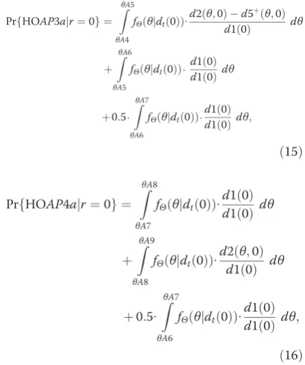
In a few cases, due to the complexity of the geometry, an approximation is applied in the estimation of the probability of HO. Figure 8 shows an example in which
the approximation is used (i.e., for the probability of HO to AP3 and AP4). These probabilities are computed as
PrfHOAP3a rj ¼0g ¼
ZθA5
θA4
fΘðθjdtð Þ0Þ:
d2ðθ;0Þ d5þðθ;0Þ
d1 0ð Þ dθ
þ ZθA6
θA5
fΘðθjdtð Þ0Þ⋅
d1 0ð Þ
d1 0ð Þdθ
þ0:5⋅
ZθA7
θA6
fΘðθjdtð Þ0Þ⋅
d1 0ð Þ
d1 0ð Þdθ;
ð15Þ
PrfHOAP4a rj ¼0g ¼ ZθA8
θA7
fΘðθjdtð Þ0 Þ:
d1 0ð Þ
d1 0ð Þ dθ
þ ZθA9
θA8
fΘðθjdtð Þ0 Þ:
d2ðθ;0Þ
d1 0ð Þ dθ
þ0:5: ZθA7
θA6
fΘðθjdtð Þ0 Þ:
d1 0ð Þ
d1 0ð Þ dθ;
ð16Þ
where in both equations the last term stands for the ap-proximation (see zoom in Figure 8).
The time Δt is selected such that, with a given prob-ability ε, it is guaranteed that the node will reach no more than one waypoint duringΔt. Since the pdf of the time between two waypoints is known [22,25], Δt is found by solving
PrfΔt≤T1þT2g≤ε; ð17Þ
Table 2 Values and numerical results for the five cases analyzed with Maple
Cases 1 2 3 4 5
Pt (1; 3π/4) (2; 7π/4) (138; 0) (1; 3π/2) (138;π/4)
WPj (63; 7π/4) (140; 7π/4) (138;π) (10; 3π/2) (70√2;π/4)
Δt(s) 10 10 60 80 10
vj(m/s) 1.4 1 2 2 1
γj 135° 135° 0° 90° 45°
xt(m) 197 2 2 1 60
xA(m) 139 142 2 141 2
Y(m) 64 138 276 9 39
Current cell 2 4 1 4 1
Pr{HOAP1}(%) 0.83 0.62 [70.06] 99.90 [100]
Pr{HOAP2} (%) [98.28] 97.43 0 0.02 0
Pr{HOAP3} (%) 0.83 0.62 0 0.04 0
Pr{HOAP4} (%) 0.06 [1.32] 29.94 [0.04] 0
Values in square brackets stand for the probability of remaining in current cell. Table 1 Probabilityεwith whichX(Δt) is smaller or equal to one
Δt(s) 50 80 90 100
whereT1 andT2 represent the timestamp (clock) of the first and of the second transitions, respectively. Table 1 shows the values for different probabilities of no more than one HO. In the cases presented below, this prob-ability is set to a minimum of 95%.
For the numerical cases,Ris set to 140 m. The mobility pattern is RWP with a uniform speed distribution between 0.7 and 2 m/s and a pause time of zero. The area is served by four APs as shown in Figure 1 (e.g., AP1 placed at point (70; 70) with respect to the centre ofA). The cell range is 70√2 m. After the equations in [22,25], the mean distance between two waypoints is equal to 126.756 m, the average time-weighted speed is 1.238 m/s and the mean time be-tween two waypoints is equal to 102.292 s.
In order to present numerical results that illustrate some interesting cases, we selected five representative cases. The selected cases are far from representing all possible scenarios but are enough to support and facili-tate a better understanding of the theoretical results. Table 2 shows the initial conditions for the cases under study. Polar coordinates are provided for Pt and WPj.
BothxtandxAare provided to show which calculation is
performed (refer to Figure 4). The probability of HO to any cell is provided. Because the probability of HO to the current cell is obviously zero, the value provided in Table 2 corresponds to the probability of remaining (i.e.,
no HO) and is enclosed in square brackets to avoid misunderstandings. The same notation is also used in Tables 3 and 4. The results are discussed after providing a better understanding of each case through Figure 9.
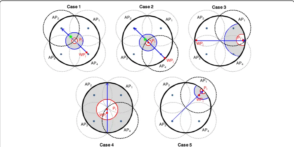
The five cases are depicted in Figure 9. The blue and red circles represent the maximum and minimum distances the node can walk if moving in any direction during Δt at maximum and minimum speeds, respect-ively. The grey area represents all the possible points that the node can reach during Δt. The blue arrow represents the current direction of the movement. The current association to a cell is marked with darker boundaries. In cases 1 and 2, the node can take any dir-ection and any speed without exiting A, while in the other cases there are directions and speeds that bring the node outside A(i.e., it changes direction and speed before exiting A). The green star represents Pt+ vj⋅Δt
(i.e., no waypoint is reached duringΔt)
In case 1, the node has just entered cell 2 and it will HO only if it reaches a waypoint. As shown in Figure 9, if the node changes direction inPt, it has roughly a 60%
of chances to HO. While moving in the same direction, the probability of HO given that node changes direction will decrease (i.e., the grey crown shown in Figure 9 gets smaller as time elapses and its center moves toward the green star); this explains the low values for the probabilities of HO. Moreover, due to the symmetry of the layout, the probabilities of HO to AP1 and AP3 are the same, while the probability of HO to AP4 is very low.
In case 2, the node is approaching the border of cell 4 toward cell 2, so HO is highly probable. Only if the node reaches the waypoint before exiting cell 4, it has some chances of remaining in the current cell or HO to AP1 or AP3. This explains the very low probabilities of HO.
In case 3, the node is reaching the boundaries ofA, so the probability of reaching the waypoint during Δt is
Table 4 Values for the other five cases analyzed with Maple and Matlab
Cases 6 7 8 9 10
Pt (105; 0.74π) (85; 0.26π) (30;π/2) (80; 3π/2) (30;π/4)
WPj (130; 0.72π) (130; 0.22π) (80;π/4) (80; 5π/4) (20; 7π/4)
Δt(s) 60 80 80 50 80
vj(m/s) 1.3 1.3 0.9 1.2 1.8
γj 295° 303° 205° 337° 79°
xt(m) 105.71 84.82 18.42 28.93 148.71
xA(m) 235.80 216.55 150.09 88.29 114.05
Y(m) 26.06 46.90 53.20 61.23 36.06
Current cell 2 1 1 3 1
Pr{HOAP1} (%) 0.75 | 0.35 [20.77] | [22.02] [3.78] | | [2.73] 0.02 | 0.01 [63.85] | [57.00] Pr{HOAP2} (%) [98.46] | [99.21] 68.20 | 70.76 90.43 | 93.66 0.14 | 0.06 19.59 | 25.30 Pr{HOAP3} (%) 0.78 | 0.44 2.04 | 0.96 2.48 | 1.20 [18.66] | [15.06] 5.35 | 3.21 Pr{HOAP4} (%) 0.01 | 0.00 8.99 | 6.27 3.31 | 2.40 81.18 | 84.87 11.21 | 14.50
Values in square brackets stand for the probability of remaining in current cell. Table 3 Average percentages of HO and no HO for the five cases simulated with Matlab
Cases 1 2 3 4 5
Pr{HOAP1} (%) 0.64 0.46 [73.80] 99.65 [100] Pr{HOAP2} (%) [98.76] 98.08 0.00 0.08 0.00 Pr{HOAP3} (%) 0.58 0.49 0.00 0.11 0.00 Pr{HOAP4} (%) 0.02 [0.98] 26.20 [0.16] 0.00
close to one. Since it is associated to cell 1 and the HO starts when the node leaves the cell, the percentage of HO to AP4 (29.94%) is lower than the percentage of no HO—recall that it is shown inside square brackets in Table 2. Even at maximum speed, the node has no time to reach cell 2 or cell 3, so the probability of HO to them is zero.
Case 4 is similar to case 2. The percentage of HO is very high (99.96%) since the node is approaching the border of its cell. Since the boundaries of cells 4 and 2 overlap at only one point (i.e., the center ofA), the node will HO to AP1 with much higher probability. On the other hand, the probabilities of HO to AP2 and AP3 only accounts for the few chances that the node has to reach the waypoint before exiting its current cell.
Finally, case 5 is similar to case 3. Again, the node will reach the waypoint because it is moving toward the boundaries of A. Because Δt is short, the node has no opportunity to leave its cell, so the probability of HO is zero. This case differs from the others in that the node is not walking through the center ofA.
6. Simulation results
The five cases analyzed are simulated with Matlab in order to evaluate the loss of accuracy produced by the necessary simplifications to the analytical model: numer-ical integration in (13), the approximation when the geometry is too complex, etc. Each simulation run consists of 5,000 samples and 10 independent repetitions
for each run are performed for each case. This simula-tion length is long enough to guarantee a confidence interval better than 95% with a margin smaller than 10% in all cases. Table 3 shows the average percentages of HO—note that the value in square brackets represents the probability of remaining in the current cell.
All of the results from simulation match the analytical results. Due to the approximation in the analysis, slight differences may be noticed among the simulation and analytical results. Still, the error in the estimation of the probability of HO in the analysis with respect to that in the simulation is always lower than 4% (case 3). Thus, the simulation validates the analytical model.
For a more comprehensive validation, other five cases (see Figure 10) are analyzed both analytically and through simulation, and the results are presented in Table 4. The error in the probability of HO or no HO is always less than 7% (case 10). These results confirm that the proposed analytical framework is valid and that the approximations and simplifications followed have only a slight impact on the results.
7. Conclusion
An analytical model for the estimation of the probability of HO to a given cell of a node moving according to the RWP mobility model has been investigated. The method is presented for a layout in which the overall area is a circle with four APs located at the corners of a square inside it. It is assumed that the position and timestamp
WPj
AP3
AP4
AP2 AP
1
AP3
AP4
AP2 AP
1
Pt
Case 1 Case 2
Case 5
WPj
Pt
AP3
AP4
AP2 AP
1
Case 3
Pt
WPj
WPj
Pt
WPj
AP1
Case 4
AP3
AP4
AP2 AP
1
AP3
AP4
AP2 AP
1
Pt
of the last waypoint are known. The model can be generalized to any symmetrical layout with overlapping areas, where the APs are placed at the corners of a regu-lar polygon (i.e., triangle, hexagon). In this article, equations are provided for the case in which the speed distribution is uniform, the pause time is zero, and propagation conditions are ideal (i.e. only path loss). Nu-merical results for several cases have been presented and compared with simulations to validate the approxi-mations assumed in the mathematical analysis. This study provides the research community with an analyt-ical framework which can improve the understanding and use of the RWP mobility model used in the majority of simulation studies with moving nodes. From a prac-tical perspective, it can be used to improve resource allo-cation in cellular networks, thus smoothing the HO procedure and improving the QoS.
Appendix 1
Expressions for the distances used in the evaluation of the probability of HO in (13) are
d1ð Þ ¼r 1
According to the geometry, other distances may be used for the evaluation of Pr{HOa}
d4ðθ;rÞ ¼1
Refer to Figure 6 for better understanding of these values.
Appendix 2
Generalization of Equations (2) to (4) in case the change of direction of movement and speed starts at S(r) leads to the following equations
xAðθtð Þr ;rÞ ¼dtð Þr:cosðθtð Þr Þ
xt θ neighboring cell AP (as two intersections may occur, the symbol ± stands for the two solutions). θ’t(r) and θ*t(r)
are derived from (5) and (6), respectively. Refer to Figure 7 for a better understanding of these values.
Competing interests
The authors declare that they have no competing interests.
Acknowledgments
This research was supported by the Spanish Government and ERDF through CICYT projects TEC2009-08198. The authors would like to thank Dr. Javier Ozón Gorriz for his suggestions and valuable help with the mathematical analysis. Part of this study has been presented at IEEE LCN conference in October, 2011 [23].
Received: 5 June 2012 Accepted: 7 January 2013 Published: 25 January 2013
References
1. A Sgora, D Vergados, Handoff prioritization and decision schemes in wireless cellular networks: a survey. IEEE Commun. Surv. Tutor.11(4), 57–77 (2009) 2. A Mishra, M Shin, W Arbaugh, An empirical analysis of the IEEE 802.11 MAC
layer handoff process. SIGCOMM Comput. Commun. Rev.33(2), 93–102 (2003) 3. H Velayos, G Karlsson, Techniques to reduce the IEEE 802.11b handoff time, in Proceedings of the IEEE International Conference on Communications, vol.7, 2004, pp. 3844–3848
4. Y Iraqi, R Baoutaba, Handoff and call dropping probabilities in wireless cellular networks, inProceedings of the IEEE International Conference on Wireless Networks, Communications and Mobile Computing, vol.1, 2005, pp. 209–213 5. WS Soh, HS Kim, QoS provisioning in cellular networks based on mobility
prediction techniques. IEEE Commun. Mag.41(1), 86–92 (2003)
6. DB Johnson, DA Maltz, Dynamic source routing in ad hoc wireless networks. Kluwer Academic Publishers Mob. Comput.353, 153–181 (1996)
7. S Kurkowski, T Camp, M Colagrosso, MANET simulation studies: the incredibles. SIGMOBILE Mob. Comput. Commun. Rev.9(4), 50–61 (2005)
8. T Ali, M Saquib, C Sengupta, Vertical handover analysis for voice over WLAN/ cellular network, inProceedings of the IEEE International Conference on Communications, ed. by, 2010, pp. 1–5
9. C Tong, JW Niu, GZ Qu, X Long, XP Gao, Complex networks properties analysis for mobile ad hoc networks. IET Commun.6(4), 370–380 (2012)
10. Q Min, R Zimmermann, An adaptive strategy for mobile ad hoc media streaming. IEEE Trans. Multimed.12(4), 317–329 (2010)
11. A Jindal, K Psounis, Contention-aware performance analysis of mobility-assisted routing. IEEE Trans. Mob. Comput.8(2), 145–161 (2009)
12. DN Alparslan, K Sohraby, Two-dimensional modeling and analysis of generalized random mobility models for wireless ad hoc networks. IEEE/ACM Trans. Netw.15(3), 616–629 (2007)
13. K Tae-Hyong, Y Qiping, L Jae-Hyoung, P Soon-Gi, S Yeon-Seung, A mobility management technique with simple handover prediction for 3 G LTE systems, inProceedings of the IEEE 66th Vehicular Technology Conference, ed. by, 2007, pp. 259–263
14. A Rojas, P Branch, G Armitage, Validation of the random waypoint mobility model through a real world mobility trace, inProceedings of the IEEE Region 10 TENCON, ed. by, 2005, pp. 1–6
15. T Camp, J Boleng, V Davies, A survey of mobility models for ad hoc network research. Wirel. Commun. Mob. Comput. (WCMC) (Special Issue on Mobile Ad Hoc Networking)2(5), 483–502 (2002)
16. F Bai, N Sadagopan, A Helmy, IMPORTANT: a framework to systematically analyze the impact of mobility on performance of routing protocols for adhoc networks. in Proceedings of the Twenty-Second Annual Joint Conference of the IEEE Computer and Communications2, 825–835 (2003)
17. TK Madsen, FHP Fitzek, R Prasad, Impact of different mobility models on connectivity probability of a wireless ad hoc network, inProceedings of the International Workshop on Wireless Ad-Hoc Networks, ed. by, 2004, pp. 120–124
18. P Lassila, E Hyytiä, H Koskinen, Connectivity properties of random waypoint mobility model for ad hoc networks, inProceedings of the Fourth Annual Mediterranean Workshop on Ad Hoc Networks, ed. by, 2005, pp. 159–168 19. V Pla, V Casares-Giner, Analytical-numerical study of the handoff area
sojourn time. in Proceedings of the IEEE Global Telecommunications Conference1, 886–890 (2002)
20. E Hyytiä, J Virtamo, Random waypoint mobility model in cellular networks. ACM/Kluwer Wirel. Netw.13(2), 177–188 (2007)
21. E Zola, F Barcelo-Arroyo, Impact of mobility models on the cell residence time in WLAN networks, inProceedings of the IEEE Sarnoff Symposium, ed. by, 2009, pp. 1–5
22. C Bettstetter, H Hartenstein, X Pérez-Costa, Stochastic properties of the random waypoint mobility model. ACM/Kluwer Wirel. Netw. (Special Issue on Modeling and Analysis of Mobile Networks)10(5), 555–567 (2004) 23. E Zola, F Barcelo-Arroyo, Probability of handoff for users moving with the
random waypoint mobility model, inProceedings of the IEEE LCN, 2011, pp. 187–190
24. C Bettstetter, G Resta, P Santi, The node distribution of the random waypoint mobility model for wireless ad hoc networks. IEEE Trans. Mob. Comput.2(3), 257–269 (2003)
25. E Hyttiä, P Lassila, J Virtamo, Spatial node distribution of the random waypoint mobility model with applications. IEEE Trans. Mob. Comput.5(6), 680–694 (2006)
26. W Yueh-Ting, H Tsung-Yen, L Wanjiun, T Cheng-Lin, Epoch, length of the random waypoint model in mobile ad hoc networks. IEEE Commun. Lett.
9(11), 1003–1005 (2005)
27. S Sangho, AG Forte, R Anshuman Singh, H Schulzrinne, Reducing MAC layer handoff latency, inIEEE 802.11 wireless LANs, in Proceedings of the ACM Second International Workshop on Mobility Management & Wireless Access Protocols, 2004, pp. 19–26
28. K Ramachandran, S Rangarajan, JC Lin, Make-before-break MAC layer handoff in 802.11 wireless networks, inProceedings of the IEEE ICC, vol.10, 2006, pp. 4818–4823
29. L Yong, G Lixin, Practical schemes for smooth MAC layer handoff in 802.11 wireless networks, inProceedings of the IEEE Computer Society International Symposium on World of Wireless, Mobile and Multimedia Networks, 2006, pp. 181–190
30. J Márquez-Barja, C Calafate, JC Cano, P Manzoni, An overview of vertical handover techniques: algorithms, protocols and tools. Elsevier. Comput. Commun.34(8), 985–997 (2011)
31. X Yan, YAŞekercioğlu, S Narayanan, A survey of vertical handover decision algorithms in Fourth Generation heterogeneous wireless networks. Elsevier Comput. Netw.54(11), 1848–1863 (2010)
32. S Lee, K Kim, K Hong, D Griffith, YH Kim, N Golmie, A probabilistic call admission control algorithm for WLAN in heterogeneous wireless environment. IEEE Trans. Wirel. Commun.8(4), 1672–1676 (2009) 33. R Ben Ali, S Pierre, On the impact of soft vertical handoff on optimal voice
admission control in PCF-based WLANs loosely coupled to 3 G networks. IEEE Trans. Wirel. Commun.8(3), 1356–1365 (2009)
34. PN Pathirana, AV Savkin, S Jha, Mobility modelling and trajectory prediction for cellular networks with mobile base stations, inProceedings of the 4th ACM International Symposium on Mobile Ad Hoc Networking & Computing, 2003,pp. 213–221
36. S Michaelis, C Wietfeld, Comparison of user mobility pattern prediction algorithms to increase handover trigger accuracy, inProceedings of the IEEE Vehicular Technology Conference, vol.2, 2006, pp. 952–956
37. MS Sricharan, V Vaidehi, A pragmatic analysis of user mobility patterns in macrocellular wireless networks. Elsevier Pervas. Mob. Comput.4(5), 616–632 (2008)
38. PS Prasad, P Agrawal, Movement prediction in wireless networks using mobility traces, inProceedings of the 7th IEEE Conference on Consumer Communications and Networking Conference, 2010, pp. 1–5 39. S Libo, D Kotz, J Ravi, H Xiaoning, Evaluating next-cell predictors with
extensive wi-fi mobility data. IEEE Trans. Mob. Comput.5(12), 1633–1649 (2006)
40. W Navidi, T Camp, Stationary distributions for the random waypoint mobility model. IEEE Trans. Mob. Comput.3(1), 99–108 (2004)
doi:10.1186/1687-1499-2013-16
Cite this article as:Zolaet al.:Forecasting the next handoff for users
moving with the Random Waypoint mobility model.EURASIP Journal on
Wireless Communications and Networking20132013:16.
Submit your manuscript to a
journal and benefi t from:
7Convenient online submission 7Rigorous peer review
7Immediate publication on acceptance 7Open access: articles freely available online 7High visibility within the fi eld
7Retaining the copyright to your article