Rupture process by waveform inversion using simulated annealing and
simulation of broadband ground motions
Yoshiaki Shiba1and Kojiro Irikura2
1Central Research Institute of Electric Power Industry, 1646 Abiko, Abiko-shi, Chiba 270-1194, Japan 2Kyoto University, Yoshida, Sakyo-ku, Kyoto 606-8501, Japan
(Received January 7, 2004; Revised May 17, 2005; Accepted May 18, 2005)
A source inversion method using very fast simulated annealing is proposed to estimate the earthquake rupture process, and associated radiation of broadband strong ground motions. We invert the displacement and velocity motions separately to estimate the spatio-temporal distributions of effective stress and moment. The developed method is applied to the near-source strong motions in the frequency range up to 5 Hz from the 1997 Izu-Hanto Toho-Oki earthquake (MJMA5.9). Results of the displacement inversion indicate that for this earthquake the seismic moment is mainly released from the shallower region and the northern area from the hypocenter. Similar results are obtained from the velocity inversion, and the variation of the effective stress also exhibits a similar behavior to the moment distribution. Based on the inversion results, we propose a characterized source model that consists of the finite number of asperities and a background area with uniform effective stresses. The broadband ground motion simulation demonstrates that the characterized source model successfully reproduces the observed ground motions in spite of the simplification of actual (inverted) source process. This suggests our proposed inversion method and source characterization process are suitable for the strong-motion prediction that reflects the high-frequency radiation from an actual earthquake.
Key words:Waveform inversion, simulated annealing, empirical Green’s function, effective stress, characterized source model.
1.
Introduction
When studying earthquake source physics it is important to reveal the rupture process that radiates seismic waves in the broadband frequency range from 0.1 to 10 Hz. Such broadband frequency motions are also of engineering inter-est for inter-estimating input ground motions used in the seismic design. Since the 1970’s a number of researchers have con-structed seismic source inversion schemes to obtain kine-matic source models from strong-motion data observed near the source region (e.g. Trifunac, 1974; Olson and Aspel, 1982; Hartzell and Heaton, 1983), revealing the complex source rupture process such as the heterogeneous slip dis-tribution. Using inversion results from many past earth-quakes, recent studies statistically examine the scaling re-lation of the “inner” fault parameters that specify the fault heterogeneity, such as the area, moment and effective stress of the asperity as well as that of the “outer” fault parame-ters that describe the overall faulting such as total rupture area and average stress drop. In these studies the asper-ity and non-asperasper-ity (background) area are categorized sys-tematically based on the objective criterion (Somervilleet al., 1999; Mai and Beroza, 2000; Miyakoshiet al., 2000). These studies are often used when source models of the sce-nario earthquakes are required for the prediction of strong ground motions.
Copy right cThe Society of Geomagnetism and Earth, Planetary and Space Sci-ences (SGEPSS); The Seismological Society of Japan; The Volcanological Society of Japan; The Geodetic Society of Japan; The Japanese Society for Planetary Sci-ences; TERRAPUB.
However, in most cases the seismic source inversions have been performed in the frequency range up to 0.5 or 1 Hz. This limitation does not reach the frequency range in which the maximum velocities and accelerations of the strong-motions are implied. This is mainly because the conventional inversion methods employ the theoretical Green’s function assuming a laterally homogeneous layered medium, which is inappropriate for evaluating ground mo-tions in the high frequency range. Furthermore, the as-sumption of a simple shape for slip velocity function and the introduction of smoothing constraints for the stability of the solution (e.g. Hartzell and Heaton, 1983) also un-derestimate the generation of high-frequency waves. Since the source models inferred from the conventional inversion methods do not include information concerning the high-frequency ground motions, it is necessary for the evalua-tion of broadband strong moevalua-tions to find the relaevalua-tionship between the asperity where the slip value is relatively large and mainly low-frequency waves are radiated and the area where mostly high-frequency motions are generated.
One way to examine these issues is to perform the inver-sion using the envelope shape of high-frequency motions instead of a waveform (e.g. Zenget al., 1993; Kakehi and Irikura, 1996). The envelope inversion eliminates the phase information of waveforms for the sake of stability of the solutions, and makes it possible to obtain information of the high-frequency radiation. Kakehi and Irikura (1996) applied the inversion procedure to envelopes of accelera-tion seismograms from the 1993 Kushiro-Oki, Japan,
quake (MW7.6) and suggested that high-frequency waves are radiated from regions that are complementary to the area of asperities that emit low frequency waves. In their formulation the inversion result exhibits the distribution of high-frequency radiation intensity. Nakaharaet al.(2002) conducted the inversion analysis using the envelopes of ob-servedS-waves that propagate through a scattering medium to estimate the high-frequency energy radiation from the moderate earthquake (MJMA6.1; MJMAmeans the magni-tude determined by Japan Meteorological Agency) in Iwate, Japan, based on the radiative transfer theory. They found that the high-frequency energy was strongly radiated from the deepest periphery of the large moment released area, estimated using the low-frequency waveform inversion. In both cases the frequency range in which the envelope inver-sions are performed is higher than 2 Hz.
On the other hand some other researchers have reported that the observed strong ground motions in the broadband frequency range from about 0.1 Hz to 10 or 20 Hz can be simulated assuming they are radiated from a large slip area. Kamae and Irikura (1998) successfully synthesized near-field strong ground motions of the 1995 Hyogo-ken Nanbu earthquake by forward modeling using the empirical Green’s function (EGF) method (Irikura, 1983, 1986). They reconstructed the source model suitable for broadband-frequency ground motions based on the model estimated from low-frequency data (Sekiguchi et al., 1996). The new model they constructed for the strong-motion simula-tion is composed of three independent patches with high stress drop located close to large moment released regions. Miyakeet al.(1999) also estimated the strong-motion gen-eration areas of two moderate earthquakes occurring in Kagoshima, Japan, on March and May 1997 by forward modeling. For the March event the strong-motion gener-ation areas they estimated agree well with the area of large dislocation deduced using the low-frequency waveform in-version by Horikawa (2001).
Apparently, the high-frequency wave radiation area de-duced from the broadband simulation does not always cor-respond to the area obtained from the envelope inversion, though the frequency ranges to which both methods are sensitive do not completely overlap. It should be noticed that the broadband simulation requires an average source model that can explain not only high-frequency motions such as accelerations and velocities, but also low-frequency displacements. By applying the inversion to the high-frequency waveforms including the phase information, it becomes possible to directly estimate the distribution of source parameters that control the high-frequency radiation, such as effective stress.
In this study we adopt very fast simulated annealing (VFSA) as an inversion algorithm to statistically find the best global solution of a nonlinear nonconvex (multimodal) problem (Ingber, 1989). VFSA is a modified algorithm on simulated annealing (SA, Kirkpatrick et al., 1983). The EGF method is used for a forward process of inversion scheme. We apply the developed method to the near-source displacement and velocity waveform data separately in the frequency range up to 5 Hz, including the frequency band in which source processes are inferred by neither the
conven-tional waveform inversion nor the envelope inversion. The spatial distributions of effective stress, seismic moment, rise time and rupture starting time are estimated in the inversion procedures. The target event we choose is the Izu-Hanto Toho-Oki earthquake of March 4, 1997 (MJMA5.9) and the observed records from its aftershock are used as the em-pirical Green’s functions. Finally we construct the char-acterized source model that consists of several rectangular asperities and background area for the target event based on the results from the velocity and displacement inversions. Characterized source models are very useful to discuss the statistical feature of earthquake source, which is easily ap-plied to the strong motion prediction. The synthetic ground motions in the frequency range up to 10 Hz are calculated from the characterized source model and the model from the velocity inversion respectively and are compared with the observed motions. We further discuss the scaling rela-tions of the asperity area and the effective stress obtained here with respect to the total seismic moment.
2.
Method
2.1 Simulated annealing
Simulated annealing (SA) is a heuristic technique to search a global minimum for the combinatorial optimiza-tion problems (Reeves, 1993). SA is based on the algorithm that simulates a physical process of heating and then slowly cooling a substance to obtain a strong crystalline structure (Metropoliset al., 1953). Atoms in a substance at high temperatures are able to move freely and keep high-energy states and when the substance is cooled slowly, the atoms line up and form a crystal that is the minimum energy for this system. By connecting these energy states with the ob-jective functions, Kirkpatricket al.(1983) proposed that the SA forms the basis of an optimization technique for combi-natorial problems. Recently SA has been introduced to the source inversion by several researchers (e.g. Ihml´e, 1996; Delouset al., 2000, 2002; Jiet al., 2002a, 2002b).
The inversion procedure based on the SA is performed as follows. First, we represent the objective function (or the misfit) to be minimized for the problem. It is usually defined as the L1 or the L2 norm of the residuals between calculated values and observed data. The model parameters are initialized randomly within the prescribed search area and the current misfit is calculated. Then, a random change from the neighborhood of the current state-space is imposed on one parameter and the corresponding change in the misfit is also evaluated. The algorithm of SA accepts not only changes that decrease misfit but also some changes that increase it. The latter are accepted with a probability based on the Boltzmann distribution.
P(T, E)=exp(−E/T) (1)
E are accepted, and thenT is lowered through the iter-ation to the value where the movement to the high-energy state is unlikely to occur. Geman and Geman (1984) proved SA guarantees an optimal solution (a global minimum) if the temperature T is decreased slower than a logarithmic manner such as,
T(k)≥ N
log(1+k) (2)
wherekis cooling time andN is the number of model pa-rameters.is the difference between the maximum energy produced by any possible configuration and the energy at the deepest local minimum. represents the height of the energy which is necessary to escape from one local minima to another one.
In this study we employ the very fast simulated annealing (VFSA) proposed by Ingber (1989). VFSA permits the temperatureT decreasing exponentially ink,
T(k)=T0exp−qkp (3)
whereT0is an initial temperature, p andq are appropriate constants. The cooling schedule of VFSA (Eq. (3)) is faster than the conventional one cited above, and it statistically finds a global minimum. The i-th model parameter mik
at cooling time k is calculated with a variable yi and the previous parametermik−1,
mi k=m
i k−1+y
i(B i−Ai)
mi
k∈[Ai,Bi],yi ∈[−1,1]
(4)
whereAiandBirespectively are the lower and upper limits
of search area for the i-th parameter. In VFSA the gen-eration of variable yi that obey the Cauchy distribution is dependent on the temperatureT at that time as follows,
yi =sgnui−1/2T(k)
(1+1/T(k))|2ui−1|−1
ui ∈U[0,1] (5)
whereui is a random variable that is generated from the uniform distribution, and thesgnfunction is 1 when the ar-gument is positive and is -1 when the arar-gument is negative. The structure of the SA algorithm is relatively simple, and there are few restrictions for the choice of the objec-tive functions because the SA does not require differential coefficients. In order to derive the high-frequency radiation based on the waveform fittings it is important to identify the amplitude and correct timing of the distinct phase implied in the observed high-frequency motions with the effective stress and rupture starting time on the fault plane. Since the rupture time has a nonlinear dependence on the wave-forms, we need to use a nonlinear inversion technique. SA or VFSA is available for such problems including strong nonlinearity, because SA has high ability to avoid the lo-cal minima and find the global minimum in the nonlinear search space.
As an alternative search algorithm based on the heuristic technique, a genetic algorithm (GA; Holland, 1975) is often applied for the inversion method in the field of geophysics. Yamanaka (2001) applied VFSA to the inversion of surface
wave phase velocity, and compared its performance with that of GA. They showed VFSA finds models that are much closer to the global minimum solution than GA within ac-ceptable computational costs. In this paper we also compare the performance of VFSA with other heuristic methods in the numerical tests.
2.2 Formulation of forward process
The application of the EGF method as a forward pro-cess of inversion is based on a review of previous studies. The idea of using observed records of a small event occur-ring near the source region of a large earthquake as an EGF was originally introduced by Hartzell (1978). Irikura (1983, 1986) combined this approach with the scaling relation-ship of source parameters (Kanamori and Anderson, 1975) and the similarity law of source spectra (Aki, 1967) to ob-tain physically reliable results when simulating strong mo-tions. Several researchers have proposed inversion proce-dures using an EGF. Fukuyama and Irikura (1989) and Fukuyama (1991) estimated the rupture starting time, mo-ment release, and rise time of the target event using an EGF and a nonlinear inversion technique, and discussed the relationship between the heterogeneous rupture pro-cess of a large earthquake and the aftershock distribution or the geological structures in the source region. Hellweg and Boatwright (1999) determined the stress drop and the rupture time of moderate earthquakes based on the filter-ing technique developed by Boatwright (1988). Mori and Hartzell (1990) used the deconvolution technique with an EGF to deduce the relative source time function to the EGF for a moderate earthquake, and estimated the slip distri-bution by using the least squares inversion. Okadaet al. (2001) and Ide (1999, 2001) investigated the rupture pro-cess of the moderate earthquake using the multiple time-window technique (Hartzell and Heaton, 1983; Ide and Takeo, 1997) and empirical Green’s functions instead of theoretical ones in order to analyze high-frequency wave-forms.
In this study we adopt the formulation of the EGF method developed by Irikura (1983, 1986). In the EGF method the fault plane of the target event is divided into sub-faults having same area. The scaling parameter N, which is a square root of the number of sub-faults, is related to the seismic moment and the effective stress as follows,
C N3= Mo mo
(6)
whereMo andmo respectively are the seismic moment of
Ci (N/ai)
ai
Fi(t) for Displacement Inversion
C1 i
C0 i (N-1)/a
Fi(t) for Velocity Inversion
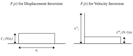
Fig. 1. A schematic illustration of the filter function F(t)used in the empirical Green’s function method. In the displacement inversionF(t)
is a boxcar function (left). The height ofF(t)is proportional to the moment density ratioCiNbetween the target event and the small event,
and its duration corresponds to the rise time of the target eventai. We
estimate the parametersCi,ai and rupture-time perturbationsi. In the
velocity inversion the filter function is composed of a delta function and a boxcar function (right). The height of a delta functionCi1is equal to the effective stress ratio.
Irikura (1989), the filter function for the displacement in-version is expressed by a boxcar function,
Fi(t)=Ci(N/ai)H(t−ti)[1−H(t−ti−ai)]
ti =(ri−r0) /β+ξi/v0+si (7)
whereCi is the weighting factor and characterizes the
av-erage effective stress ratio of thei-th sub-fault of the target event to the element event. ThenCiN represents the ratio
of the released moment from thei-th sub-fault to that of the element event. ai is the rise time. r0 andri respectively
are the distance from the hypocenter andi-th sub-fault to the observation station.ξiis the distance from the
hypocen-ter toi-th sub-fault andv0is the assumed constant rupture velocity. si is perturbation from the rupture timeξi/v0. β is theS-wave velocity. H(t)represents the Heaviside step function, which is 1 fort ≥0, and is 0 fort <0. Since the integration of Fi(t)with respect tot is equal to CiN, the
convolution with the filter functionFi(t)givesCiN times
larger spectral amplitude in the lower limit of frequency, assuring the suitable moment ratio between each sub-fault of the target event and the element event. In the displace-ment inversion we estimate three model parametersCi,ai
andsi. The total moment of the target eventMois estimated
by
Mo=moN M
i=1
Ci, (8)
whereMrepresents the number of sub-faults and is usually equal toN2, though in case of source inversionM is often set to be larger thanNto retain the appropriate search space for the inversion procedure.
For the representation of high-frequency radiation, the use ofFi(t)defined in Eq. (7) is inappropriate, because the
Fourier spectrum of a boxcar function decays in proportion toω−1, whereωdenotes the angular frequency. Theω−2 model providing the shape of source spectrum based on the scaling law (Aki, 1967) requires that the high-frequency asymptote of Fi(ω)goes toCi (Irikura, 1986). To satisfy
this condition Irikura (1986) proposed a new type of the fil-ter function to which the Dirac delta functionδ(t)is added as follows,
Fi(t)=Ci{δ(t−ti)
+[(N−1)/ai]H(t−ti)
·[1−H(t−ti−ai)]}. (9)
A time integral of Fi(t)agrees with the released moment
ratio CiN in Eq. (9) as well as in Eq. (7). Furthermore
the amplitude of the Fourier spectrumFi(ω)becomesCiin
the high-frequency asymptote due to the contribution of the delta function. Therefore the filter function (9) ensures the scaling relation between the target and the element event in both the high frequency and low frequency range. It also should be noticed that the synthesized slip velocity time function of the target event using Eq. (9) roughly re-sembles the slip velocity derived from the dynamic source rupture modeling (e.g. Day, 1982), so that the calculated ground motions are expected to preserve physically accept-able characteristics in the broadband frequency range. In this study we modify Eq. (9) for the velocity inversion to estimate the amplitude of the delta function and that of the following boxcar function individually,
Fi(t)=Ci1δ (t−ti)
+Ci0[(N−1) /ai]
·H(t−ti)[1−H(t−ti−ai)]. (10)
In the velocity inversion we estimate C0
i, C1i and the
rupture-time perturbationsi (see Eq. (7)) ofi-th sub-fault.
The model parameterC1
i is interpreted to stand for the
in-tensity of high-frequency radiation andCi0 represents the
amplitude of intermediate and low frequency motions. The rise timeai is specified by using the results from the
dis-placement inversion. Note that the effective stress ratio of thei-th sub-fault of the target event to the element event is equivalent toCi1, which is the coefficient of the delta
func-tion, and the moment ratio between them is derived from the time integral of Eq. (10), i.e.C1
i +Ci0(N−1)
In both the displacement and velocity inversion, we im-pose a constraint on the rupture-time perturbationsi to
sup-press the instability of solutions. Following Yoshida and Koketsu (1990) and Horikawa (2001), the constraint for the rupture propagation is expressed as
∇2s
i =0, (11)
where∇2is a discrete Laplacian operator. The VFSA in-version is performed by minimizing the misfit to data and the constraint shown in Eq. (11). A relative weighting fac-torW is introduced into the minimization process to obtain the best-balanced solution that satisfies both realistic rup-ture propagation and small misfit to waveforms. The resul-tant inversion criteria can be represented as
E+W·
i
∇2s
i =minimum, (12)
whereEdenotes the misfit, which is given by the L1 or L2 norm of the residuals between the synthetic and observed ground motions. For one waveform the misfits using the L1 normEL1and the L2 normEL2are described as
EL1=
ntm
i=1
|us(ti)−uo(ti)|
ntm
i=1
(uo(ti))2
1/2
EL2=
ntm
i=1
(us(ti)−uo(ti))2
ntm
i=1
(uo(ti))2,
139°00' 139°15' 139°30' 34°45'
35°00' 35°15'
0 10 20
km
Izu Peninsula
MNZHTS ATM
KWN
YAS Target Event
Element Event
135°E 140°E
34°N 36°N 38°N
Central Japan
Fig. 2. Map showing the epicenter of the target event (large open star), el-ement event (small open star) and other aftershocks (open circles). The focal mechanisms of the target and element events are also shown. The open triangles indicate the strong motion stations on the rock outcrops used in this study.
where us and uo are the synthetic and observed ground
motions respectively. ntm is the number of data points. In later section we will compare the ability of finding true parameters forEL1andEL2in the numerical tests.
Though many researchers have adopted a spatial smooth-ing constraint for slips or slip velocities together with that for time variables, we do not employ additional constraints to ensure free spatial distribution of other model parame-ters. Only the nonnegative constraints for the moment and the effective stress are included in the choice of lower limit of search area,Ai in Eq. (4).
3.
Data
We applied the developed VFSA inversion to strong-motion data recorded at bedrock stations during the 1997 Izu-Hanto Toho-Oki earthquake (MJMA 5.9). The target event was the largest within the moderate earthquake swarm occurring over a several-day period in March, 1997 (JMA, 1997). We used the records from the following small event (MJMA4.9) for the empirical Green’s function (the element event). In general high-frequency radiation from the seis-mic source can be investigated more minutely by choosing a smaller EGF, because the size of sub-fault becomes smaller. However, the number of observed records from such a small event is not often enough for the inversion analysis. Fur-thermore, the lower limit of the frequency band available for the inversion analysis is restricted by the signal-to-noise ratio of the observed EGF. In the EGF method the high-frequency radiation whose wavelength is shorter than the grid-size for the inversion is contained in the element event itself, hence it is represented statistically by superposing the employed EGF. In Fig. 2 the epicenters of the target event, element event and other aftershocks occurring within one day are shown with the distribution of observation stations we analyzed. Their hypocentral locations were determined by JMA and the focal mechanisms were published by F-net
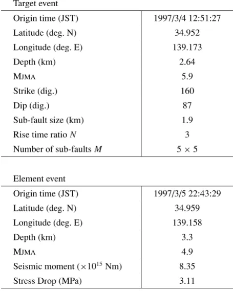
Table 1. The initial source parameters of the target and element events used for the inversion.
Target event
Origin time (JST) 1997/3/4 12:51:27
Latitude (deg. N) 34.952
Longitude (deg. E) 139.173
Depth (km) 2.64
MJMA 5.9
Strike (dig.) 160
Dip (dig.) 87
Sub-fault size (km) 1.9
Rise time ratioN 3
Number of sub-faultsM 5×5
Element event
Origin time (JST) 1997/3/5 22:43:29
Latitude (deg. N) 34.959
Longitude (deg. E) 139.158
Depth (km) 3.3
MJMA 4.9
Seismic moment (×1015Nm) 8.35
Stress Drop (MPa) 3.11
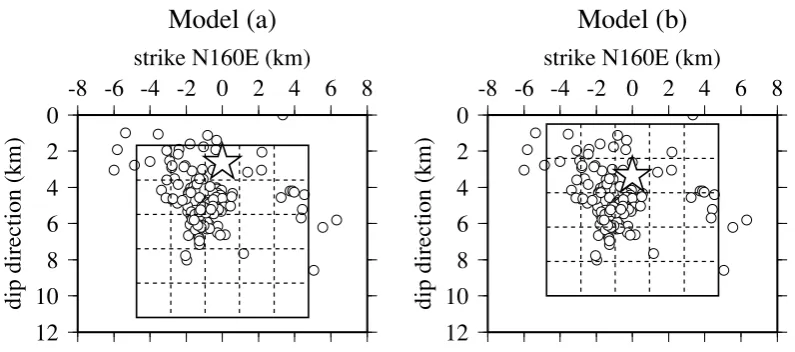
(Fukuyamaet al., 1998). All of the stations are on rock out-crops with three-component force-balanced accelerometers operated by the Central Research Institute of Electric Power Industry (CRIEPI). The observed acceleration records were band-pass-filtered from 0.4 to 5 Hz, and then numerically integrated to obtain data for the velocity and displacement inversions. We prepared two initial fault models as shown in Fig. 3 based on the aftershock distribution. The source parameters for the inversion are shown in Table 1. The S wave velocity of 3.2 km/s in the source region was esti-mated by taking an average of theSwave velocity structures proposed by Takeo (1988). From the aftershock distribution in depth we determined the upper limit of the seismogenic zone to be the depth of 0.5 km. In model (a) we located the hypocenter in the middle of the strike direction and in the shallowest part along the dip direction as seen in Fig. 3. In model (b) the hypocenter is located on the deep adjacent mesh. In this model the edge of the fault reaches the up-per border of the seismogenic zone. Then the focal depth, which is assumed to be located on the center of the mesh, is set on the slightly deeper position due to the fixed size of the sub-fault that is equivalent to the fault dimensions of the element event. We performed the VFSA inversion us-ing these two initial models and adopted the better model by comparing the fit between the synthetic ground motions and the observed ones.
0
2
4
6
8
10
12
dip direction (km)
-8 -6 -4 -2 0
2
4
6
8
strike N160E (km)
Model (a)
0
2
4
6
8
10
12
dip direction (km)
-8 -6 -4 -2 0
2
4
6
8
strike N160E (km)
Model (b)
Fig. 3. Assumed fault models for the inversion analysis. Star indicates the hypocenter. Open circles show the hypocenters of aftershocks determined by JMA.
we obtained the rough estimates of the fault radii of these events. The rise time ratioN, which is equal to the scale pa-rameter shown in Eq. (6), is directly determined from the ra-tio of fault size between the target and element events. The number of sub-faultsM was set to be(N +2)2 by adding columns and rows around theN2fault area.
The radiation patterns were not corrected in this analy-sis because the fault orientation of the element event was similar to that of the target event. However for the stations located close to the extension of nodal planes of the fault, the radiation patterns of two horizontal components are cal-culated for the target and element event respectively. The effect of the radiation pattern on the inversion result is dis-cussed in later sections. The frequency dependence of the attenuation factor for the S-waves, QS(f), is assumed as
QS(f) = 130f0.7 for f ≥ 1 Hz, which is obtained by
Kinoshita (1994) in the crust of the Southern Kanto area including the source region in this study.
Since all model parameters except for the rise time are the ratios to those of the element event in our inversion scheme, it is necessary to accurately determine the values of these parameters for the element event in advance in order to discuss the physical faulting process of the target event. The seismic moment of the element eventmois estimated from
the low-frequency asymptote of the displacement source spectrum obtained from the spectral inversion analysis. The total seismic moment of the target event is also deduced from this analysis, so we can use it for the comparison with results of inversion. The stress drop σ of the element event is estimated assuming a circular fault (Eshelby, 1957) as follows,
σ = 7 16
mo
r3 (14)
whererdenotes the source radius deduced from the spectral inversion. We assume that the effective stress σe related
to high-frequency motions is equal to the stress dropσ (Brune, 1970, 1971).
4.
Inversion Results
4.1 Numerical tests
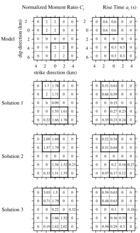
To examine the validity of the developed inversion method, we applied it to the ground motions synthesized from an artificial fault model. Two different fault models were prepared for the displacement inversion and the ve-locity inversion, respectively as shown in the upper part of Figs. 4 and 5. In the lower part of Figs. 4 and 5 we show the best three solutions out of ten attempts using the appropriate control parameter for inversion procedure discussed later in this section. The model for the displacement inversion in-cludes two distinct asperity areas of the same released mo-ment. The moment release from the background area is set to be zero. The rise time of the shallow asperity is twice as long as that of the deep asperity. It should be noticed that we display the weightCias the “normalized” moment ratio
instead ofCiN in the left column of Fig. 4. WhenCi =1
over the entire fault of the target event, the total released moment corresponds to the value expected from the scaling relation of seismic source (Kanamori and Anderson, 1975) with uniform effective stress (or stress drop), therefore the distribution ofCi indicates the discrepancy in the moment
release from a homogeneous source of the same magnitude. For the velocity inversion there are also two distinct asperi-ties on the model fault. As seen in Fig. 5 the shallow asper-ity shows half the effective stress compared with the deep asperity, but twice as large as the parameterCi0that controls
the amplitude of boxcar function. Furthermore the effective stress ratioCi1 is doubled at one mesh within each
asper-ity. A constant rupture velocity of 0.8βis assumed for both models. The station distribution and other initial parameters required for the inversion procedure are equivalent to those in the actual situation introduced above. Note that for the fault geometry and the hypocenter location we adopted the parameters for the assumed fault model (b).
syn-2
Displacement inversion using artificial source model
Model
Normalized Moment Ratio Ci
2
Fig. 4. Spatial distributions of the normalized moment ratio and the rise time of the artificial fault model used in the numerical test for the displacement inversion (upper two figures), and the three best inversion results with smaller L1-norm misfits (lower six figures). Two squared areas enclosed by thick solid lines indicate asperities with different rise times. The moment is released from only the asperity areas in this test model.
thetic data set was prepared. Since our concern isS-waves, we used the two horizontal components. Each seismogram was band-pass-filtered from 0.1 to 5 Hz, and the sampling interval was reduced to 0.05 s in order to save computation time. The search areas of model parameters are shown in Table 2. We determined the search area of rupture-time per-turbationsifrom the variation in the rupture velocity. When
v1andv2are the lower and upper limits of rupture velocities respectively, the search area ofsiis obtained by
s1i ≤si ≤s2i
s1i =ξi/v2−ξi/v0 s2i =ξi/v1−ξi/v0,
(15)
whereξiis the distance from the hypocenter to thei-th
sub-fault andv0is the constant rupture velocity of the assumed model as seen in Eq. (7). Several experimental attempts are performed before the inversion in order to determine the parameters for the cooling schedule. We have to choose the initial temperatureT0, the coefficients pandq that control
2
Velocity inversion using artificial source model
Model
Effective Stress Ratio C1 i
Fig. 5. Spatial distributions of the effective stress ratioC1
i and the
pa-rameterC0
i that is proportional to the amplitude of the boxcar function
used for the numerical test in the velocity inversion (upper two figures), and the three best inversion results with smaller L2-norm misfits (lower six figures). The assumed source model consists of two distinct asper-ity areas (squares enclosed by thick solid lines) and only the peak slip velocity is doubled at one mesh within each asperity displayed as the gray-shaded area.
Table 2. Search areas of model parameters in numerical tests. Displacement inversion
10-2 10-1 10-1 100 101 102
Misf
it
0 20000 40000 60000
Count
Velocity Inversion (q=1.0)
p=0.4 p=0.5 p=0.6
p=0.7 p=0.8 p=0.9
10-1 100 100 101 102
Misf
it
0 20000 40000 60000
Count
Displacement Inversion (q=1.0)
p=0.4 p=0.5 p=0.6
p=0.7 p=0.8 p=0.9
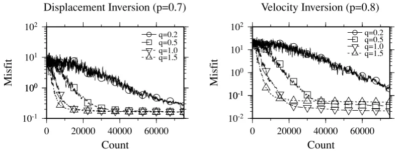
Fig. 6. Variation of misfits with differentpvalues in Eq. (3). Note that the misfits displayed here are the L1 norms for the displacement inversion and the L2 norms for the velocity inversion, respectively. We employed these norms in the following practical analyses.
10-2 10-1 10-1 100 101 102
Misf
it
0 20000 40000 60000
Count
Velocity Inversion (p=0.8)
q=0.2 q=0.5 q=1.0 q=1.5
10-1 100 100 101 102
Misf
it
0 20000 40000 60000
Count
Displacement Inversion (p=0.7)
q=0.2 q=0.5 q=1.0 q=1.5
Fig. 7. Variation of misfits with differentqvalues in Eq. (3). The selected norms for the misfits are same as Fig. 6.
such that,
T0= E +sd(E). (16) To determine the lowering speed of the temperature, the test runs were made with changing the value of the coefficients p andq in Eq. (3). Figure 6 shows the variations of mis-fits with lowering the temperature in the displacement and velocity inversions when the coefficient p in the cooling schedule is varied from 0.4 to 0.9 with fixedq of 1.0. We can see the amplitude of the misfit function drops rapidly just after the beginning of iteration as the value of p in-creases. However as the iteration count progresses the mis-fit with the cooling schedule using large pof 0.9 does not reduce sufficiently due to few opportunities to accept new parameters that might lead to the global optimal solution. Hereafter we use p = 0.7 for the displacement inversion and 0.8 for the velocity inversion. In Fig. 7 we show the case of varyingqwith fixed p. The cooling schedule using q = 1.0 is the most suitable in the velocity inversion for the search of the optimal solution, and that withq ≥ 0.5 is appropriate in the displacement inversion. Therefore we useq =1.0 hereafter for both inversions. Finally we deter-mined the critical temperatureTcfollowing the suggestion
of Ihml´e (1996) and Gibert and Virieux (1991),
Tc=Kvar(noi se)=Kvar(E) (17)
whereKis an appropriate constant determined through
sev-eral test runs. Once the temperature reachesTc, the
parame-ter search is repeated with remaining the temperature atTc.
As pointed out by Mosegaard and Tarantola (1995), when the definition of misfit is the L2 norm andK in Eq. (17) is equal to 1, the iterative search at the critical temperature Tc in the Metropolis algorithm provides the model
sam-pling according to the posterior probability distribution in the Bayesian approach with Gaussian noise. In this study we assumeK ranges from 0.1 to 0.5 to ensure reliable con-vergence. The algorithm terminates when a preset number of iterations have been completed. In this study the number of iterations at the same temperature was set to 10 until the temperature is lowered toTc. Further the total number of
iterations was set to 74,000. Since the number of model pa-rameters is 25 (the number of sub-faults)×3 (Ci,ai andsi
for the displacement inversion, andCi0,Ci1andsifor the
ve-locity inversion)−1 (siat the rupture starting mesh) = 74,
1,000 iterations were performed for each parameter. The appropriate weight for the smoothing constraint on the rup-ture time was examined by performing some preliminary inversions. In practice the solution of the VFSA inversion is not completely independent on the initial values for gener-ation of random numbers due to finite itergener-ations. Therefore we performed 10 inversions with different initial values, and examined the dispersion of solutions and the discrepancy from the true models.
0 1 2 3
1 2 3 4 5
Displacement inversion (artificial model)
L1 inversion
Normalized Moment Ratio Ci
0
Normalized Moment_Ratio Ci
0
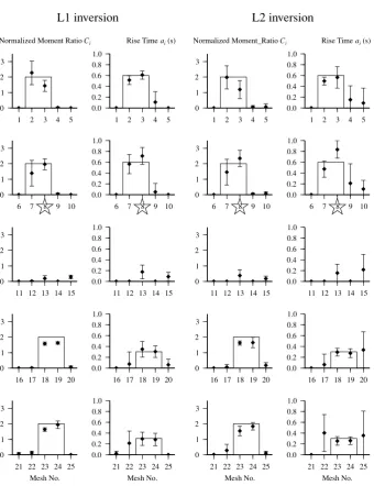
Fig. 8. Averages and the standard deviations of estimated parameters in the displacement inversion, which are obtained from 10 attempts with different initial values in random number generators. Horizontal axis indicates the mesh number of the target fault, measured from the northern shallowest mesh to the strike direction. 8th mesh marked with star indicates the hypocenter. Continuous solid lines show the parameter distribution of the assumed model.
parameters estimated from the displacement inversion in Fig. 8, and those from the velocity inversion in Fig. 9, along with the initially assumed models drawn by solid lines. We found that the source parameters estimated from both inver-sions agree well with those of the models. In particular the results from the velocity inversion reproduce the model al-most precisely and the standard deviations are very small, especially in case using the L2 norm as the misfit function. While the estimated parameters in the displacement inver-sion show larger fluctuations compared to the case of ve-locity inversion. The incorrect values of rise times are ob-tained at surrounding meshes of asperities. This is because the variation of rise time is insensitive to that of the syn-thetic ground motion when the released moment at the cor-responding mesh is small. At the outside of asperity area,
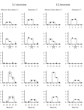
the displacement inversion minimizing the L2 norm yields larger estimation error of rise time than that minimizing the L1 norm, as shown in Fig. 8. On the other hand the velocity inversion using the L2 norm minimization provides better solutions than that with the L1 norm in estimation of the effective stress at the deep asperity.
0
Velocity inversion (artificial model)
L1 inversion
Effective Stress Ratio C1 i
Effective Stress Ratio C1 i
Fig. 9. Averages and the standard deviations of estimated parameters in the velocity inversion. 8th mesh marked with star indicates the hypocenter. Continuous solid lines display the parameter distribution of the assumed model.
102
0 20000 40000 60000
Count
0 20000 40000 60000
Count
Displacement Inversion
10-2 10-1 10-1 100 101 102
Min. misfit
0 20000 40000 60000
Number of generated models VFSA MA IM GA
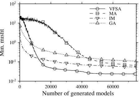
Fig. 11. Minimum misfit values obtained from the four different search al-gorithms, which are Metropolis algorithm (MA), iterative improvement method (IM) and genetic algorithm (GA). Horizontal axis indicates the number of generated models (i.e. calculation of ground motions)
of the misfits with different initial values is rather small. Temperature reaches the critical pointTc at about the 20th
lowering in the displacement inversion and the 30th lower-ing in the velocity inversion in this numerical test, which correspond with 14,800 and 22,500 iterations respectively as indicated by arrows in Fig. 10.
Finally we attempted the same numerical tests by us-ing the other heuristic techniques, which are the conven-tional Metropolis algorithm (MA), the iterative improve-ment method (IM) and the genetic algorithm (GA). The conventional MA means simulated annealing that searches a new parameter from the full search area uniformly. IM is the algorithm which accepts a new random parameter if and only if it provides a superior (small misfit) model. The number of model generations in GA is set to agree with that in VFSA. The elite selection to 10% of the best individ-uals and the dynamic mutation fluctuating from 1 to 10% are introduced in GA. The resultant minimum misfit val-ues obtained from these four search algorithms are shown in Fig. 11 as a function of the number of examined mod-els. As seen in Fig. 11 the misfit of VFSA falls slower than GA and IM until about 10,000 model generations due to the almost pure random search at high temperature. Af-ter that, however, VFSA can find betAf-ter solutions compared with other methods as indicated by the lower misfit values. Since the iterative improvement moves to the model with smaller misfit straightforwardly, the misfit value reduces very rapidly in the early stage. But this method is likely to converge towards the local minima (Mosegaard and Vester-gaard, 1991). The reduction of the misfit is slowest in con-ventional MA until more than half of the model realizations in the total iteration schedule are performed because of very slow cooling schedule. MA samples the parameters assum-ing a uniform distribution in the model space, so that milder cooling step is necessary to attain the global minimum. The performance of GA is not so good in this numerical test. Generally GA can find the area where the global minimum exists more easily than the family of SA. While once the point near the global minimum is found, the neighborhood search algorithm like VFSA is better for the local search
Displacement (cm) at KWN_NS (0.4 - 5Hz)
Obs. 2.07
Model (a) 0.71
Model (b) 1.70
0 1 2 3 4 5 6
Time (sec)
Fig. 12. Displacement waveforms on the NS component at KWN. Top trace shows the observed waveform. Middle and bottom traces show the synthetic waveforms from the model (a) and the model (b) respectively.
Table 3. Search areas of model parameters in application to the target event.
Displacement inversion
C a(s) v/β
0.0–2.0 0.0–1.0 0.55–0.8
Velocity inversion
C0 C1 v/β
0.0–2.0 0.0–5.0 0.55–0.8
(e.g. Reeves, 1993).
4.2 Application to the 1997 Izu-Hanto Toho-Oki
Earthquake
We applied the VFSA inversion to the strong-motion records from the 1997 Izu-Hanto Toho-Oki Earthquake of MJMA 5.9. First we determined the suitable initial fault model from the models (a) and (b) as shown in Fig. 3. When the location of the initial fault model is inappropri-ate, ground motions at the station close to the fault such KWN are not often represented well. Here we performed the displacement inversion with two assumed fault models and compared the synthetic ground motions at KWN with observed one. In Fig. 12 we show the displacement mo-tions of the NS component at KWN. Obviously the syn-thetic displacement motion based on the fault model (b) agrees well with the observed one compared to the syn-thetic motion with the model (a). In fact the inverted source model by using model (b) releases a large moment from the shallowest area as discussed later, which is not included in the model (a). Consequently we adopted the initial fault model (b) in this study.
Table 4. Comparison of the total seismic moment of the target event obtained by the VFSA displacement inversion with those determined from spectral analysis and by other researchers (F-net and Kikuchi (1997, on the web site))
This study Spectral analysis F-net Kikuchi (1997)
Total moment (Nm) 1.31×10¹⁷ 1.75×10¹⁷ 2.09×10¹⁷ 1.00×10¹⁷
-2 0 2 4 6
dip direction (km)
-4 -2 0 2 4
strike direction (km)
Displacement Inversion
Moment Density
Solution 1
-2 0 2 4 6
-4 -2 0 2 4
0.77 0.09 0.21 0.38 0.87 0.27
Rise Time (s)
-2 0 2 4 6
-4 -2 0 2 4
Solution 2
-2 0 2 4 6
-4 -2 0 2 4
1 0.41 0.94 0.38 0.75
-2 0 2 4 6
-4 -2 0 2 4
Solution 3
0 1 2 3 4 5 6
(*1015Nm/km2)
-2 0 2 4 6
-4 -2 0 2 4
0.72 0.98 1
0.33
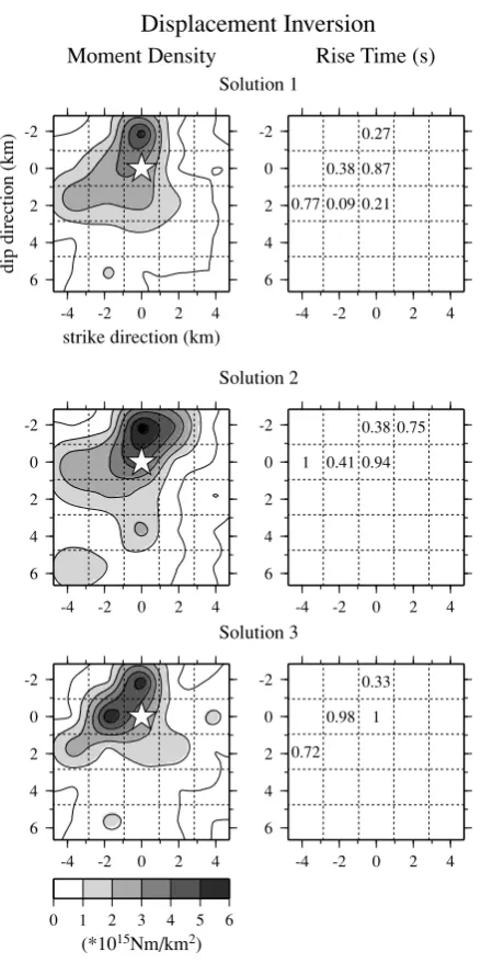
Fig. 13. The best three source models regarding the distributions of moment density and rise time for the target event for 10 solutions of the VFSA displacement inversions. Values of rise time are given only for the sub-faults where more than twice the average moment is released. An open star shows the hypocenter.
S waves. We found that the radiation patterns of the EW component at KWN from more than half of the sub-faults of the target event show the opposite sign to that from the element event. To correct such differences in the sign of radiation patterns we performed the displacement inversion with changing the sign of the element waveform of the EW component at KWN. However the resultant synthetic mo-tion of the target event shows an almost reverse trace to the observed one, suggesting that the sign of the radiation
pat-Displacement (cm) 0.4 - 5Hz
NS ATM
0.17
0.15
HTS
0.58
0.65
KWN
2.07
1.70
MNZ
0.20
0.22
YAS
0.48
0.51
EW 0.15
0.10
1.10
0.99
1.65
1.13
0.36
0.32
0.29
0.21
0 1 2 3 4 5 6 Time (s)
0 1 2 3 4 5 6 Time (s)
Fig. 14. Comparison of synthetic and observed displacement waveforms. Solid lines show the observed waveforms and broken lines denote syn-thetic ones. Numbers above the waveforms are the peak values of ob-served motions and those below the waveforms are the peak values of synthetics, respectively.
tern from the target event should be same as that from the element event for suitable waveform fittings. Since the EW component at KWN is close to the nodal for the target and element event, a small change in the fault geometry and/or lateral heterogeneity of subsurface structure might change the sign of radiation patterns. We also attempted the dis-placement inversion without the EW component of KWN. The obtained moment distribution is roughly coincides with the inversion results obtained by using full data. However the variance of the rupture times inferred from the inversion with different initial values becomes large due to a decrease in the number of data. Therefore we did not remove the EW component of KWN in the following analysis.
0 10 20
Frequenc
ypercent
0 2 4 6 8 10 12 14
Moment Density (*1015Nm/km2)
Displacement Inversion
0 10 20
Frequenc
ypercent
0.0 0.2 0.4 0.6 0.8 1.0
Rise Time (s)
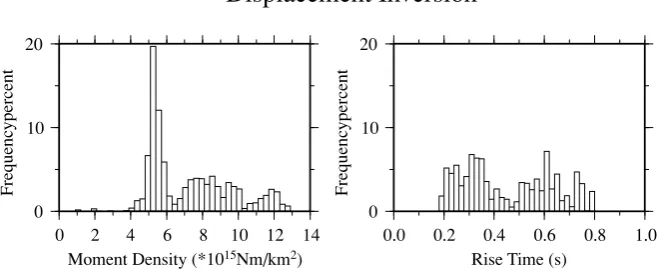
Fig. 15. Histograms of the a posteriori parameter distributions at the asperity mesh located just above the hypocenter sampled just belowTcfrom 10
displacement inversions. About 7,000 sampled models are plotted.
the end of inversion. The best three source models in Fig. 13 show similar moment distributions. The large moment re-leased area is located in the shallow region just above the hypocenter and extends to the northern area (the left direc-tion in the figure) of the hypocenter. The rise time distribu-tion ranges from 0.3 to 1 second, showing large variadistribu-tions. In Table 4 we compare the total seismic moment obtained from the best three inversion results on average with the re-sults from other studies, which are the spectral inversion (in this study) and the moment tensor inversion reported by F-net (Fukuyamaet al., 1998) and Kikuchi (1997, on the web site). Our estimated seismic moment coincides well with other results. Figure 14 shows the synthetic displacement motions calculated from the best source model with the ob-served ones. The fit between them is generally good.
To see the most frequently sampled values in the inver-sion procedure, we show in Fig. 15 the histograms of the pa-rameter distributions at the asperity mesh located just above the hypocenter, which are sampled just below the critical temperature from 10 inversions. The histogram of model parameters is interpreted as the marginal a posteriori distri-butions (Mosegaard and Tarantola, 1995; Ihml´e and Ruegg, 1997), and gives us the information of the reliability and the resolution of estimated solutions. As seen in Fig. 15, the histogram of sampled moment densities in the displace-ment inversion shows a distinct peak near 5×10¹⁵Nm/km2, while the sampled value of rise time distributes more exten-sively.
For the velocity inversion we also show the three best models within 10 inversions in Fig. 16. The rise times at the large moment-released meshes are fixed by averaging the three best results of displacement inversion. For other meshes where small or almost no moments are released in the displacement inversion, we assumed the constant value of 0.5 second. The moment distribution derived from the velocity inversion roughly corresponds to that from the dis-placement inversion shown in Fig. 13. However the total amount of the released moment is about 40% smaller than the result from the displacement inversion. The reason is that the velocity inversion might be insensitive to the low-frequency components that are directly related to the re-leased moment, because the VFSA algorithm tends to fit higher-frequency motions more correctly in the velocity
in--2 0 2 4 6
dip direction (km)
-4 -2 0 2 4
strike direction (km)
Velocity Inversion
Effective Stress
Solution 1
-2 0 2 4 6
-4 -2 0 2 4
Moment Density
-2 0 2 4 6
-4 -2 0 2 4
Solution 2
-2 0 2 4 6
-4 -2 0 2 4
-2 0 2 4 6
-4 -2 0 2 4
Solution 3
0.0 0.5 1.0 1.5 2.0 2.5 3.0 (MPa)
-2 0 2 4 6
-4 -2 0 2 4
0 1 2 3 4 5 6
(*1015Nm/km2)
0 10 20 30 40
Frequenc
ypercent
0 1 2 3 4 5
Effective Stress (MPa)
Velocity Inversion
0 10 20 30 40
Frequenc
ypercent
0 2 4 6 8 10
Moment Density (*1015Nm/km2)
Fig. 17. Histograms of the a posteriori parameter distributions at the asperity mesh located just above the hypocenter sampled just belowTcobtained
from 10 velocity inversions. The number of sampled models is roughly the same as that in the displacement inversion.
version. The distribution of the effective stress is similar to that of the moment release in the velocity inversion. This implies that radiation of the high-frequency waves share common areas with the release of the large moment, i.e. asperity.
In Fig. 17 we show the histograms of the parameter dis-tributions obtained from the velocity inversion at the same mesh as the case of the displacement inversion. The dis-tribution of the moment density is relatively well centered at the value being generally consistent with those estimated from the displacement inversion in Fig. 15, though the ef-fective stress shows two peaks in the histogram.
Velocity (cm/s) 0.4 - 5Hz
NS ATM
0.90
0.64
HTS
4.88
4.75
KWN
10.14
7.60
MNZ
3.94
1.49
YAS
2.47
3.84
EW 0.77
0.37
4.39
4.54
10.23
6.37
2.26
1.28
2.50
2.09
0 1 2 3 4 5 6 Time (s)
0 1 2 3 4 5 6 Time (s)
Fig. 18. Comparison of synthetic and observed velocity waveforms. Solid lines show the observed waveforms and broken lines denote synthetic ones. Numbers above the waveforms are the peak values of observed motions and those below the waveforms are the peak values of synthet-ics, respectively.
Figure 18 compares the synthetic velocity motions from the source model with the smallest misfit and the observed ones. The estimated source model reproduces the velocity motions rather well though it is still difficult to fit the high-frequency signals accurately.
Figure 19 shows the distribution of the rupture-time per-turbationsi for both the displacement and velocity
inver-sions. We see the perturbation of the rupture time from the initial model with the constant rupture velocity is small and the rupture propagation is very smooth on the fault plane of the target event.
5.
Discussion
5.1 Selection of the type of norm for calculation of
misfit
In this study we minimize the L1 norm for the evalua-tion of the misfit during the displacement inversion. Gener-ally the L2 norm is often employed for the measurement of misfit between observed data and models in the inversion procedure, because the L2 norm is used for maximizing the likelihood function that obeys the Gaussian distribution (Duijndam, 1988). It is well known that the Gaussian distri-bution approximates closely the behavior of errors of many measurements in physical problems. On the other hand the L1 norm is more robust having the property to be less sensi-tive to large outliers than the L2 norm. For instance Das and Kostrov (1990) solved the source inversion by using the lin-ear programming method with the minimization of the L1 norm. They also evaluated the L2 norm and the L∞norm (Chebyshev norm), and confirmed the L2 norm behaves in a similar manner than the L1 norm in their inversion proce-dure. It should be noted that minimizing the L1 norm sig-nifies finding a median out of the noisy data, while the L2 norm minimization produces a mean value (Claerbout and Muir, 1973). In Fig. 20 we show the histogram of resid-uals derived from the L1 norm fitting in the displacement inversion and that from the L2 norm fitting in the veloc-ity inversion respectively. Here the residual is normalized with the standard deviationσ such as (uS(t)−uO(t)) /σ
for each station and component, whereuS anduO are the
synthetic and observed motions as shown in Eq. (13). In Fig. 20 both residuals obey the normal distribution with zero mean, which indicates the selection of the L1 norm as well as the L2 norm is appropriate in our problem.
0 5 10 15
Frequenc
ypercent
4 3 2 1 0 1 2 3 4
Residual
Residual distribution using the L1 norm in displacement inversion
0 5 10 15
Frequenc
ypercent
4 3 2 1 0 1 2 3 4
Residual
Residual distribution using the L2 norm in velocity inversion
Fig. 20. Histogram of residuals derived from the L1 norm fitting in the displacement inversion (left) and that from the L2 norm fitting in the velocity inversion (right).
-0.2 -0.1 0.0 0.1 0.2
T
ime Perturbations (s)
1 2 3 4 5
Vel. Inversion Disp. Inversion
Inversion Results
-0.2 -0.1 0.0 0.1 0.2
6 7 8 9 10
-0.2 -0.1 0.0 0.1 0.2
11 12 13 14 15
-0.2 -0.1 0.0 0.1 0.2
16 17 18 19 20
-0.2 -0.1 0.0 0.1 0.2
21 22 23 24 25 Grid No.
Fig. 19. Distribution of the rupture-time perturbationsi for both the
displacement and velocity inversions for the three best inversion results. Horizontal axis indicates the mesh number of the target fault, measured from the northern shallowest mesh along the strike direction.
major discontinuity. In our problem the L2 norm is appro-priate for fitting the wave portion near the peak amplitude, and the L1 norm is able to fit the total waveforms at some cost to accuracy near the peak values. Since the rise time is considered to be more sensitive to total waveforms than individual peak amplitudes for long-period waves, it is ap-propriate to use the L1 norm for the displacement inversion. In contrast, it is important for the velocity inversion to fit several distinct peak amplitudes of high-frequency velocity motions in order to infer the spatio-temporal distribution of effective stress as well as the seismic moment. Therefore the L2 norm is better for the velocity inversion, though few differences were seen between the results of the L1 and L2 norm minimization in the numerical test.
5.2 Characterization of source model and broadband
ground motion simulation
-2 0 2 4 6
dip direction (km)
-4 -2 0 2 4
strike direction (km) 0.00 1.12 0.00 0.00 0.00 0.00 0.41 0.82 0.41 0.00 2.71 2.03 2.35 1.15 0.00 0.90 2.69 2.91 0.00 0.00 0.00 0.63 5.28 0.00 0.00
Solution 1
1.99 1.00 0.31 0.00 0.00 0.25 0.00 2.38 0.00 0.00 1.48 2.08 1.30 0.00 0.01 2.83 2.86 4.75 0.64 0.00 0.00 0.59 6.32 3.78 0.00
Solution 2
Displacement Inversion
0 1 2 3 4 5 6 7
Moment Density (*1015Nm/km2)
0.01 1.14 0.63 0.00 0.00 0.00 0.07 0.81 0.03 0.00 2.50 0.70 1.42 1.78 0.00 0.00 5.56 2.97 0.00 1.21 0.00 0.77 5.42 0.00 0.06
Solution 3
Fig. 21. Total rupture area and the area of asperity for the characterized source model identified from the three best solutions of the displacement inversion. The areas enclosed with the thick lines indicate the areas of asperity. The edges divided by the broken lines are removed to define the rupture area of the characterized source model.
modeling technique and found the sizes and positions of the strong motion generation area estimated from the strong ground motions in the broadband frequency range coincide with those of the characterized asperity derived from the low-frequency ground motions. Here we characterize the spatial variations of effective stress and released moment for the target event estimated by the VFSA inversion. Then the validity of the characterization scheme is confirmed by comparing the synthetic ground motions using character-ized source model with the observed ones in the broadband frequency range up to 10 Hz, which is often required for an engineering purpose. The scaling relation of characterized source parameters with seismic moment is also compared with other studies.
First we identify the total rupture area and the asper-ity area of the target event from the moment distribution obtained using the displacement inversion. Somervilleet al. (1999) proposed the way of determination of the ob-jective rupture area by removing the edges with small slip values from the heterogeneous slip model. They also de-fined the identification of asperity based on the relative slip value in each sub-fault. We apply the criterion presented by Somervilleet al.(1999) correspondingly to characterization of our inversion results, though we use the moment distribu-tion as a substitute for the slip distribudistribu-tion. Figure 21 shows the total rupture area and the area of asperity we identified from the three best results of the displacement inversion. The edge column on the right side in Fig. 21 is trimmed due to small moment release. Then the rupture area of the characterized model is defined. The area of asperity is de-termined as the area composed of four sub-faults located near the hypocenter. The ratio of the asperity area to total rupture area is 0.2, which is consistent with the empirical relation of 0.22 deduced by Somervilleet al.(1999). Fig-ure 22 shows the relation between the area of asperity and the seismic moment of the target event and the comparison with the scaling proposed by Somervilleet al.(1999) and Miyakeet al. (2003). Note that the scaling relation pro-posed by Miyakeet al.(2003) provides the strong motion
generation area with respect to the seismic moment as men-tioned above. Here we adopt the seismic moment of the target event determined from the moment tensor inversion by F-net (Fukuyamaet al., 1998). The relation of asperity area to seismic moment shows a good agreement with the empirical scaling relations by Somervilleet al.(1999) and Miyakeet al.(2003).
100
101
101
102
103
104
Combined Area
of Asperities
(km
2)
1016 10101717 1018 1019 1020 Seismic Moment (Nm)
Somerville et al. (1999) Miyake et al. (2003) This study
Fig. 22. Relation between the area of asperity and the seismic moment. Solid star shows the relation of the target event found in this study. Open diamonds and triangles are the combined area of asperities (Somerville
et al., 1999) and the strong motion generation areas (Miyakeet al., 2003), respectively. Broken line shows the scaling relation proposed by Somervilleet al.(1999).
ra-EW
Acceleration (cm/s/s)Obs. 50.50
Velocity (cm/s)
4.45
Displacement (cm)
1.12
VIM 39.49 5.42 1.11
CM1 34.71 4.48 1.11
CM2 27.41 4.67 1.13
0 1 2 3 4 5
Time (s)
0 1 2 3 4 5
Time (s)
0 1 2 3 4 5
Time (s)
NS
Acceleration (cm/s/s)Obs. 60.01
Velocity (cm/s)
5.26
Displacement (cm)
0.58
VIM 48.44 5.54 0.76
CM1 40.31 3.75 0.81
CM2 32.97 3.98 0.80
Fig. 23. Comparison between the synthetic ground motions from three source models and the observed ground motions at HTS. Number above each trace shows the peak value. “VIM” indicates the source model directly using the result of the velocity inversion. “CM1” is the characterized source model composed of only asperities, and “CM2” is that including asperities and background area.
Table 5. Parameters of the characterized source model for the target event.
Asperity Background
Na Ca NT a Nb Cb NT b
2 0.46 3.30 4 0.098 3.62
tioC1
i as,
Aa0 a0
= Na
L×NWa
i=1
Ci1
2 1/2
, (18)
whereAa
0anda0are the high-frequency amplitude level of the acceleration spectrum for the asperity of the target event and the element event, respectively. Na
L and NWa indicate
the scaling factors concerning the fault length and width of the asperity area that we initially estimated. For the characterized source modelAa0/a0is equal toCaNa, where
Ca and Na denote the effective stress ratio and the fault
dimension ratio between the characterized asperity and the element event. Then we obtain the following relation,
CaNa =
Na L×NWa
i=1
Ci1
2 1/2
. (19)
The moment ratio of the asperity to the element event is represented usingCaandNaas follows,
CaNa3=
Na L×NWa
i=1 M i o
mo
(20)
where Moi is the released moment from thei-th sub-fault
andmo is that from the element event. From Eqs. (19) and
(20) the uniform effective stress ratioCa and the fault
di-mension ratio Na of the characterized asperity to the
el-ement event are estimated. (It should be noticed that the characterized asperity area N2
a not necessarily corresponds
to the initial guess ofNLa×N a
W.) Here we assume the area
of high effective stress for the target event corresponds to the asperity area deduced from the results of the displace-ment inversion. Then we obtainCa = 0.46 and Na = 2,
which results in the equal area to the initial assumption. The effective stress ratioCbon the background area
sur-rounding the asperity is given by the following equations,
CbNb3=
i∈/Na L×NWa
i M
i o
mo
Nb =
N2−N2
a
(21)
whereN andNbare the scaling factor concerning the fault
dimension of the total rupture area and background area re-spectively. The addition of seismic momentsMi
oin Eq. (21)
is carried out at the sub-faults except for the initially as-sumedNLa×N
a
Wasperity.
The total amount of the seismic moment is corrected using the results from the displacement inversion due to the underestimation of the seismic moment in the velocity inversion. The correction is made by changing the scaling factor concerning the slip duration time (or rise time) as follows,
CaNa2NT a=
Na L×NWa
i=1 M i od
mo
(22)
whereNT ais the rise time ratio between characterized
as-perity and element event.Modi denotes the seismic moment
of thei-th sub-fault estimated from the displacement inver-sion. Though Eq. (22) is valid for the characterized asperity area, a similar relation is valid for the background area to estimate the rise time ratioNT b.
The estimated parameters for the characterized source model of the target event,Ca,NaandNT afor the asperity
andCb,Nb and NT bfor the background area, are
0.1 1 10
(cm/s)
0.1 1
Period (s) ATM NS
0.1 1
ATM EW
1 10
0.1 1
HTS NS
0.1 1
HTS EW
1 10 100
0.1 1
KWN NS
0.1 1
KWN EW
1 10
0.1 1
MNZ NS
0.1 1
MNZ EW
1 10
0.1 1
YAS NS
0.1 1
YAS EW
Obs. VIM CM1 CM2
Fig. 24. Pseudo velocity response spectra with 5% damping calculated from the observed and three synthetic ground motions.
the velocity inversions. We obtain the effective stress ratio at asperity of 0.46 and that in the background area of 0.098. So the ratio of effective stress between the characterized as-perity and the background area become approximately 0.2, which is as twice large as the solutions of numerical simula-tions based on the dynamic rupture model with single asper-ity (Irikura, 2004). Since the effective stress of the element event is estimated as 3.11 MPa (see Table 1), the effective stress on the asperity of the characterized source model be-comes 1.43 MPa, which is very small compared with the average value of 10.5 MPa deduced by Irikura (2004). The moment release from the asperity occupies 52% of the total moment, which is slightly larger than the empirical relation of 44% (Somervilleet al., 1999) and the dynamic solution of single asperity model of 45.5% (Irikura, 2004), which might be due to the rough spatial division of the fault plane. We calculate synthetic ground motions in the frequency range from 0.4 to 10 Hz with the EGF method based on three source models, i.e. the model using the results of ve-locity inversion directly, characterized source model with only the asperity and characterized source model with as-perity and background area. The rise time is fixed to be 0.5 second over the entire fault and constant rupture ve-locity of 0.65 times theS wave velocity is assumed for all source models. Figure 23 shows the comparison between the synthetic ground motions from three source models and the observed ground motions at HTS as an example. The fit between the synthetic and observed ground motions are generally good for their peak values and envelope shapes, though detailed waveforms do not agree completely.
The pseudo velocity response spectra calculated from the observed and three synthetic ground motions are shown in Fig. 24. On the EW components at the stations of KWN and YAS the synthetic ground motions from all three mod-els underestimate the low-frequency amplitudes compared with the observed motions as seen in Fig. 24. The EW com-ponents at KWN and YAS are nearly nodal for theS-waves from both the target and element events. As discussed be-fore the radiation pattern on the EW component at these stations will vary with the position of the sub-fault for the target event if the hypocentral distance is short. The effect of the radiation pattern from the target event is therefore smoothed for the stations located in the direction of the fault normal, and hence the synthesized motion will be underes-timated when the radiation pattern for the element event is small. The NS component at MNZ also shows a large dis-crepancy in the spectral amplitude between synthesized and observed motions. MNZ is relatively far from the hypocen-ter and is located in the direction close to the strike of the both events. Accordingly the amplitude of the synthesized ground motion on the NS component at MNZ is further sen-sitive to a small difference in the fault geometry between the target and small events. In fact, we can see the radiation pattern on the NS component for the element event is very small compared with that for the target event at the azimuth of MNZ. This might be the reason for the underestimation of the NS component at MNZ.
0.5 0.6 0.7 0.8 0.9 1.0
CrossCorrelations
Vel. Dsp. Env.
0.8 0.9 1.0 1.1 1.2 1.3
L2 Residuals
Vel. Dsp. Env. 1.4
VIM CM1 CM2
Fig. 25. Cross-correlations (left) and residuals (right) between the synthetic and observed waveforms.
with acceleration envelopes. The decrease of the cross-correlations and the increase of the residuals caused by the characterization of the source model from the velocity in-version are rather small except for the residual of the veloc-ity motions, which is the objective function to be minimized during the VFSA inversion procedure.
6.
Conclusions
A source inversion using very fast simulated annealing (VFSA) with the empirical Green’s function method was proposed for estimating the rupture process radiating broad-band ground motions. This inversion algorithm allows us to separately estimate the spatial distributions of the ef-fective stress and seismic moment with the rupture time by inverting the velocity ground motions in the frequency range up to 5 Hz. From the displacement motions the re-leased moment, rise time and rupture time are estimated. The developed inversion method was applied to the strong-motion data from the 1997 Izu-Hanto Toho-Oki earthquake (MJMA5.9). Results of the displacement and velocity inver-sion exhibit the similar distribution of the seismic moment, in which the large moment released area is located in the shallow part just above the hypocenter and extends a little deeper to the northern area. The distribution of the effec-tive stress deduced from the velocity inversion is similar to that of the moment release, suggesting that radiation of the high-frequency waves share common areas with the release of the large moment, i.e. asperity. We further displayed the procedure for constructing the characterized source model from the spatial distributions of the effective stress and the seismic moment obtained from the VFSA inversions. The validity