HIPSTER - A Python package for particle physics analyses

HIPSTER

A Python package for particle physics analyses

1_{School of Physics and Astronomy, Queen Mary University of London, G O Jones Building, 327 Mile} End Road, London, E1 4NS, UK

Abstract. HIPSTER (Heavily Ionising Particle Standard Toolkit for Event Recognition) is an open source Python package designed to facilitate the use of TensorFlow in a high energy physics analysis context. The core function-ality of the software is presented, with images from the MoEDAL experiment Nuclear Track Detectors (NTDs) serving as an example dataset. Convolutional neural networks are selected as the classification algorithm for this dataset and the process of training a variety of models with different hyper-parameters is detailed. Next the results are shown for the MoEDAL problem demonstrating the rich information output by HIPSTER that enables the user to probe the per-formance of their model in detail.

1 Introduction

Machine learning has evolved as a field over many years, with the Fisher Discriminant [1] from 1936 forming the basis of the perceptron [2] an early neural network style model from 1958. In particle physics machine learning has been used as a tool since the 1990s [3] in some form or another, mostly for solving classification problems. Boosted decision trees emerged as the favourite algorithm for this task and though these algorithms are still competitive with many more modern techniques the recent explosion of so-called deep learning presents new options. The rise of deep learning as a field of research has been met with adoption of its techniques within many other areas, which has in turn led to a large increase in the number of open source machine learning frameworks available. It has also led to a diversification in the number of applications of machine learning algoritms that are no longer limited to solving classification or regression problems. Importantly from the perspective of particle physics many of these tools are developed and maintained by teams that are very well funded, typically leading to a faster pace of development and quality of documentation than could be afforded in our field.

We present HIPSTER as a means of interfacing with these modern machine learning tools. HIPSTER is a wrapper around TensorFlow [4] and also offers a number of features

that facilitate its easier use. These features largely rely on the NumPy package for numerical Python [5]. Functionality is designed with the data analysis of nuclear track detectors (NTDs) in mind, specifically those deployed at the MoEDAL experiment [6] at the Large Hadron Collider (LHC) [7], however there also exists minimal functionality for more traditional high energy physics problems, for example the Higgs Kaggle Challenge [8]. The design philsophy

of HIPSTER is to learn as much from the field of machine learning research as possible whilst keeping interfaces to particle physics specific software such as ROOT [9] separate from the core code. Section 2 will outline the core functionality of the package as well as several modular interfaces to external packages, and will be followed by examples from the MoEDAL NTD analysis in Section 3.

2 Features of the HIPSTER library

One significant feature of HIPSTER is to build deep learning models from a user supplied configuration. In this sense the library serves as an interface to other machine learning tools. Two models, the multi-layer perceptron (MLP) and convolutional neural network (CNN), will be detailed in the following subsections. There are far more extensive libraries in existence such as Keras [10] that allow users to build models using a TensorFlow back-end, however HIPSTER was designed with the MoEDAL NTD analysis in mind.

The NTD analysis relies heavily on the processing of images. The interfaces to CNN types models are therefore the most complete in the library. The interfaces to both the CNNs and other models are implemented with best practice procedure from the deep learning com-munity in mind. Specific elements of the package that may be different to traditional image processing include the functionality to keep track of geometric features specific to the analy-sis of NTDs, namely the multiple layers of an NTD and the different sides of those layers.

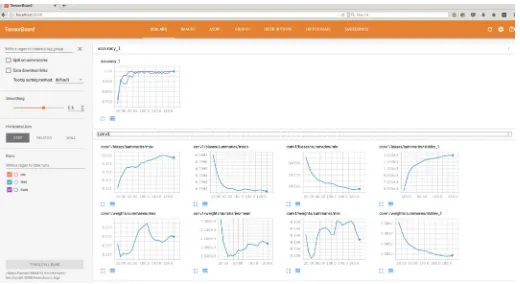
There are also some more general tools that have been adopted for instance TensorBoard. TensorBoard is a suite of tools used to debug and diagnose the performance of a models built in TensorFlow, HIPSTER models automatically include the necessary summary operations to ensure that the training can be easily visualised. Figure 1 shows an example of the kind of information that one can view in TensorBoard after training a model with HIPSTER. A model instantiated in HIPSTER will output the required files to view the TensorBoard output automatically, whereas by using TensorFlow in its original form one would have to manually call the necessary functions in their model in order to output the correct information.

Figure 1: A screen capture of the TensorBoard output from a model trained in HIPSTER on simulated NTD data, viewed in a web browser.

2.1 Multi-layer perceptrons

of HIPSTER is to learn as much from the field of machine learning research as possible whilst keeping interfaces to particle physics specific software such as ROOT [9] separate from the core code. Section 2 will outline the core functionality of the package as well as several modular interfaces to external packages, and will be followed by examples from the MoEDAL NTD analysis in Section 3.

2 Features of the HIPSTER library

One significant feature of HIPSTER is to build deep learning models from a user supplied configuration. In this sense the library serves as an interface to other machine learning tools. Two models, the multi-layer perceptron (MLP) and convolutional neural network (CNN), will be detailed in the following subsections. There are far more extensive libraries in existence such as Keras [10] that allow users to build models using a TensorFlow back-end, however HIPSTER was designed with the MoEDAL NTD analysis in mind.

The NTD analysis relies heavily on the processing of images. The interfaces to CNN types models are therefore the most complete in the library. The interfaces to both the CNNs and other models are implemented with best practice procedure from the deep learning com-munity in mind. Specific elements of the package that may be different to traditional image processing include the functionality to keep track of geometric features specific to the analy-sis of NTDs, namely the multiple layers of an NTD and the different sides of those layers.

There are also some more general tools that have been adopted for instance TensorBoard. TensorBoard is a suite of tools used to debug and diagnose the performance of a models built in TensorFlow, HIPSTER models automatically include the necessary summary operations to ensure that the training can be easily visualised. Figure 1 shows an example of the kind of information that one can view in TensorBoard after training a model with HIPSTER. A model instantiated in HIPSTER will output the required files to view the TensorBoard output automatically, whereas by using TensorFlow in its original form one would have to manually call the necessary functions in their model in order to output the correct information.

Figure 1: A screen capture of the TensorBoard output from a model trained in HIPSTER on simulated NTD data, viewed in a web browser.

2.1 Multi-layer perceptrons

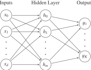
Multi-layer perceptrons are models that fit the structure outlined in figure 2. The architecture of MLP models is defined by a number hyper-parameters, for example the number of hidden layers in the network or the number of nodes each layer contains. In general when the number

.

.

.

.

.

.

.

.

.

Inputs Hidden Layer Outputs

Figure 2: A basic neural network containing an input layer ofdnodes corresponding to data of dimensionalityd, a hidden layer ofmhidden unitshiand an output layer ofKpredictive

unitsyi.

of hidden layers is larger than two the network could be referred to as a deep neural network with no specific distiction between a neural network (NN) and a deep neural network (DNN). When every node in a given layer is connected to every node in the layers adjacent to it the network may also be described as a fully connected network (FCN). Furthermore feedfoward NNs are models in which the graph of nodes has no loops, that is to say data flows exclusively through the graph in one directions, forward. Developed in the 1980s, Recurrent NNs [11–13] are NNs that where nodes such that loops are formed, specifically Long Short-Term Memory (LSTM) NNs [14] have recently gained popularity in particle physics [3], though they are not included in HIPSTER currently there are plans for these models to be included in the future. In HIPSTER MLPs of arbitrary size can be created by callingDNNwith options specifying the network inputs, number of predictive classes and the network architecture. Additionally one may pick from a number of different activation functions and choose whether or not to use dropout [15], a technique to prevent neural networks from overfitting. Two example functions existMLP2andMLP5which demonstrate the functionality of theDNNfunction. The options of MLP models are interfaced by theMLPTrainingOptionsclass which keeps track of all of the relevant parameters and allows them be altered at the desire of the user.

2.2 Convolutional Neural Networks

C O N V

C O N V

C O N V

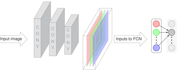
Input image Inputs to FCN

Figure 3: The structure of a basic convolutional neural network. Decreasing size of con-volutional layers indicates sub-sampling (e.g. maxpool). Red, green and blue layers could match their corresponding layers of an RBG image or represent any layer in an arbitrary voxel structure.

networks [18], whilst these are not currently available in HIPSTER efforts to include this functionality in a release are on-going.

CNN models can be created in HIPSTER with theCNNfunction which acts like theDNN function with a different set of options. Currently the type of convolutional layer supported

istf.nn.conv2d, the TensorFlow two dimensional convolution operation. In addition the

software currently assumes that a layer of sub-sampling e.g. maxpooling will follow each convolutional layer. In practice one may wish to forgo sub-sampling if an image is already small or simply to experiment with different network architectures. Whilst this achievable by taking the trivial sub-sample in the step where sub-sampling is assumed, in future more flexi-bility will be included with regards to specifying the order of the layers and their types. Fully connected layers can be added to the end of the network with the same implementation as a DNNstyle network. In order to match the size of the final layer of the feature extraction part of the network to the input size of the classification portion a functionget_FCinputNodes exists. The options for a CNN are interfaced by theCNNTrainingOptionsclass which is analogous toMLPTrainingOptions.

2.3 General Features

As well as the classes for handling model options and functions for implementing DNN and CNN models HIPSTER comes with a number of other tools that assist in the building, training and evaluation of machine learning models. A few of these are highlighted here. In order to facilitate easier training of DNNsTrainDeepNetworkexists as a one line call to build and train a deep network. Model building for both DNNs and CNNs is made easier with the use of reconfigure and auto-configure functions that can be called after a check is carried out on a set of training options to verify is they would build a valid network or not. An example of such a check is ensuring that the sub-sampling layer in a CNN does not fail due to input array size being too small, this would be automatically detected by the options class.

C O N V C O N V C O N V

Input image Inputs to FCN

Figure 3: The structure of a basic convolutional neural network. Decreasing size of con-volutional layers indicates sub-sampling (e.g. maxpool). Red, green and blue layers could match their corresponding layers of an RBG image or represent any layer in an arbitrary voxel structure.

networks [18], whilst these are not currently available in HIPSTER efforts to include this functionality in a release are on-going.

CNN models can be created in HIPSTER with theCNNfunction which acts like theDNN function with a different set of options. Currently the type of convolutional layer supported

istf.nn.conv2d, the TensorFlow two dimensional convolution operation. In addition the

software currently assumes that a layer of sub-sampling e.g. maxpooling will follow each convolutional layer. In practice one may wish to forgo sub-sampling if an image is already small or simply to experiment with different network architectures. Whilst this achievable by taking the trivial sub-sample in the step where sub-sampling is assumed, in future more flexi-bility will be included with regards to specifying the order of the layers and their types. Fully connected layers can be added to the end of the network with the same implementation as a DNNstyle network. In order to match the size of the final layer of the feature extraction part of the network to the input size of the classification portion a functionget_FCinputNodes exists. The options for a CNN are interfaced by theCNNTrainingOptionsclass which is analogous toMLPTrainingOptions.

2.3 General Features

As well as the classes for handling model options and functions for implementing DNN and CNN models HIPSTER comes with a number of other tools that assist in the building, training and evaluation of machine learning models. A few of these are highlighted here. In order to facilitate easier training of DNNsTrainDeepNetworkexists as a one line call to build and train a deep network. Model building for both DNNs and CNNs is made easier with the use of reconfigure and auto-configure functions that can be called after a check is carried out on a set of training options to verify is they would build a valid network or not. An example of such a check is ensuring that the sub-sampling layer in a CNN does not fail due to input array size being too small, this would be automatically detected by the options class.

Several types of model evaluation are available within the package. Inbuilt support for TensorBoard allows the user to view many useful metrics in their web-browser. This includes the evolution of the accuracy and loss of a model over time as well as more complex informa-tion. The response of the learned filters can be viewed directly for a subset of the training data

for CNN type models. TensorBoard support includes Embedding Projector functionality that allows the user to visualise high dimensional data interactively, though the meaning of these embeddings is highly dependent on the problem being tackled. The aforementioned tools are useful for diagnosing the behaviour of a model during training. HIPSTER is also capable of outputting information that helps to determine the success of a model once trained. The most commonly used of these metrics is the receiving operator characteristic curve (ROC curve) and the area under the curve (AUC).

3 Example application

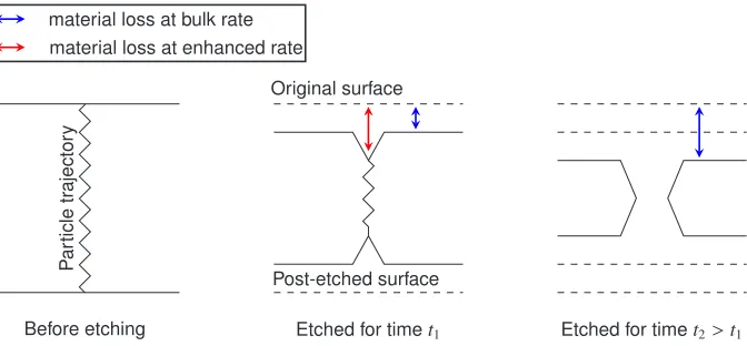
The MoEDAL experiment [6] coniststs of a number of detectors designed to probe for beyond the standard model (BSM) physics. One such method is an array of Nuclear Track Detec-tors (NTDs) each element of which consists of a number of alternating layers of CR39 and Makrofol polymer kept in an aluminium housing. This array is sensitive to highly ionising particles that cause breaks in the intra-molecular bonds as they pass through the bulk of the polymer. The breaks in these chains of molecules cause erosion of material when exposed to a hot sodium hydroxide solution to be accelerated. The effect is that the otherwise uniform loss of material across the surfuce of a polymer sheet is increased in the local area surround-ing the past trajectory of the particle, formsurround-ing what is known as an etch pit as in figure 4. The signatures that the experiment searches for are when these areas of damage are aligned

material loss at enhanced rate material loss at bulk rate

P ar ticle trajector y Before etching Original surface

Etched for timet1 Post-etched surface

Etched for timet2>t1

Figure 4: Sketch of cross sectional view of a polymer sheet at different stages of the etching process.

across a number of layers from the same module indicating that a highly ionising particle penetrated the stack. After being exposed to the LHC conditions the NTDs are scanned to form a dataset of images. The search for etch pits within these images is a fundamental task is the analysis of MoEDAL NTD data. It is this search that has largely informed the design of the HIPSTER.

Figure 5: Twelve images taken from the training dataset in the example application. The network was trained to classify whether or not an image contained an etch pit.

early versions of the etching process and scanning techniques, it also is very low in statis-tics with only several hundred labelled examples of about 40×40 pixels each. Despite a suboptimal dataset the CNN was able to achieve 80% accuracy, although the variance of this result on more data, were it available, is expected to be high due to the small training set. The advances in the etching and scanning techniques are expected to yield much improved results in terms of accuracy and variance.

For the results reported only a single side of each piece of polymer was considered, how-ever the HIPSTER library is equipped to deal specifically with the case in which both sides are considered (as well as accounting for relationships between different layers in the stack).

A full analysis is expected to be completed by the MoEDAL collaboration in the future in which these extra details will be considered, making full use of the HIPSTER library. In the minimal example presented tweaking of model configurations between training sessions was made easier with the use of HIPSTER. In particular due to a benchmarking mode in hipster that outputs training meta-data in a particular structure for each training. This data includes TensorFlow checkpoint files to restore the model, the files necessary for viewing the Ten-sorBoard output, as well as some replicated information from TenTen-sorBoard output to simple text files (to make easier automating the process of evaluating many models at once), for ex-ample model accuracy, time to train, whether or not early termination was invoked and the hyper-parameter configuration of the trained model.

3.1 Availability and the future

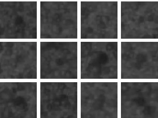
Figure 5: Twelve images taken from the training dataset in the example application. The network was trained to classify whether or not an image contained an etch pit.

early versions of the etching process and scanning techniques, it also is very low in statis-tics with only several hundred labelled examples of about 40×40 pixels each. Despite a suboptimal dataset the CNN was able to achieve 80% accuracy, although the variance of this result on more data, were it available, is expected to be high due to the small training set. The advances in the etching and scanning techniques are expected to yield much improved results in terms of accuracy and variance.

For the results reported only a single side of each piece of polymer was considered, how-ever the HIPSTER library is equipped to deal specifically with the case in which both sides are considered (as well as accounting for relationships between different layers in the stack).

A full analysis is expected to be completed by the MoEDAL collaboration in the future in which these extra details will be considered, making full use of the HIPSTER library. In the minimal example presented tweaking of model configurations between training sessions was made easier with the use of HIPSTER. In particular due to a benchmarking mode in hipster that outputs training meta-data in a particular structure for each training. This data includes TensorFlow checkpoint files to restore the model, the files necessary for viewing the Ten-sorBoard output, as well as some replicated information from TenTen-sorBoard output to simple text files (to make easier automating the process of evaluating many models at once), for ex-ample model accuracy, time to train, whether or not early termination was invoked and the hyper-parameter configuration of the trained model.

3.1 Availability and the future

This article is based on the a pre-release version of the HIPSTER library, which is currently not available for installation by the general public. There are plans to make the library avail-able on the Python Package Index in the future. The current dependencies of the software are as follows: TensorFlow [4], NumPy [5], Pillow [19] and matplotlib [20]. Features interfacing with ROOT are dependent on the ROOT package for data analysis [9] and those interfacing with data from LabVIEW are dependent on the npTDMS [21] package.

As the MoEDAL NTD analysis continues HIPSTER will also evolve to meet the needs of the group, this will define the priorities of the development team going forward. Nevertheless the developers also seek to add implementations of popular machine learning algorithms as already eluded to even if they have no immediate relation to the MoEDAL NTD analysis. There is also an interest to enable HIPSTER to wrap around Keras models as these models can be imported to TMVA [22] which then makes them compatible with large analysis frameworks such as those used on the ATLAS and CMS collaborations.

This publication uses data generated via the Zooniverse.org platform, development of which is funded by generous support, including a Global Impact Award from Google, and by a grant from the Alfred P. Sloan Foundation.

This authors would specifically like to thank the following University of Alabama undergrad-uate students Zach Buckley, Sarah Deutsch, Thomas (Hank) Richards, Cameron Roberts, Andie Wall and Alex Watts, for their work in labelling data.

The authors would like to thank the Nvidia corporation for providing hardware that was used to carry out this research.

The authors would like to thank the Science and Technology Facilities Council (UK) for providing funding for this research.

References

[1] Fisher, R. A., The Use Of Multiple Measurements In Taxonomic Problems, Annals of Eugenics,7, 179–188 (1936) doi:10.1111/j.1469–1809.1936.tb02137.x

[2] Rosenblatt, F., The Perceptron: A Probabilistic Model For Information Stor-age And Organization In The Brain, Psychological Review 65(6), 386–406 (1958) doi:10.1037/h0042519

[3] Albertsson, K. and others, Machine Learning in High Energy Physics Community White Paper, (2018) doi:10.1088/1742–6596/1085/2/022008

[4] Abadi, M. and others, TensorFlow: Large-scale machine learning on heterogeneous sys-tems, (2015), Software available from tensorflow.org arXiv:1603.04467

[5] Travis E., O.A guide to NumPy(Trelgol Publishing, USA, 2006) ISBN:9781517300074 [6] Pinfold, J., The MoEDAL experiment at the LHC, EPJ Web of Conferences145, 12002

(2017)

[7] Evans, L. and Bryant, P., LHC Machine, Journal of Instrumentation 3, (2008) doi:10.1088/1748–0221/3/08/S08001

[8] Adam-Bourdarios, C. and others, The Higgs boson machine learning challenge, Journal of Machine Learning Research Workshop and Conference Proceedings42, 19–55 (2015) doi:10.1088/1742–6596/664/7/072015

[9] Brun, R. and Rademakers, F., ROOT — An Object Oriented Data Analysis Frame-work, Nucl. Inst. & Meth. in Phys. Res. A38981–86 (1997), See also http://root.cern.ch/

doi:10.1016/S0168–9002(97)00048-X

[10] Chollet, F. and others, Keras, (2015), See also https://keras.io

[12] Jordan, M. I., Serial order: A parallel distributed processing approach. Technical Report 8604, (1986) doi:10.1016/S0166–4115(97)80111–2

[13] Elman, J. L., Finding structure in time. Cognitive science, 14(2), 179211, (1990) doi:10.1016/0364–0213(90)90002-E

[14] Hochreiter, S. and Schmidhuber, J., Long Short-Term Memory, Neural Computation,9 (8), 1735–1780, (1997) doi:10.1162/neco.1997.9.8.1735

[15] Srivastava, N. and others, Dropout: A Simple Way To Prevent Neural Net-works from Overfitting Journal of Machine Learning Research 15, 1929–1958 (2014) doi:10.1007/978–3–642–46466–9_18

[16] Fukushima, K., Neocognitron: A Self-organizing Neural Network Model for a Mech-anism of Pattern Recognition Unaffected by Shift in Position, Biological Cybernetics36,

193–202 (1980) doi:10.1007/BF00344251

[17] LeCun, Y. and others, Object Recognition with Gradient-Based Learning, (1999) doi:10.1007/3–540–46805–6_19

[18] Sutskever, I. V., O. & Le. Q. V., Sequence to Sequence Learning with Neural Net-works, Proc. Advances in Neural Information Processing Systems27, 3104-3112 (2014) arXiv:1409.3215v3

[19] Clark, A. and others, Pillow — The friendly PIL fork, (2016) doi:10.5281/zenodo.44297

[20] Caswell, T. and others, matplotlib: plotting with Python, (2018) doi:10.5281/

zen-odo.1482098

[21] Reeve, A. and others, npTDMS, https://github.com/adamreeve/npTDMS

[22] Hoecker, A. and others, TMVA — Toolkit for Multivariate Data Analysis, PoS ACAT