Article
A
M
odified
C
ell-
B
ased
S
train
S
moothing
for
M
aterial
N
onlinearity
ChangkyeLee1andSundararajanNatarajan2*
1
2
3
4
5
6
7
8
9
10
11
12
1 UniversityCoreResearchCenterforDisaster-freeandSafeOceanCityConstruction,Dong-AUniversity,
49315,Busan,Korea;[email protected](C.L.)
2 IntegratedModellingSimulationLab,DepartmentofMechanicalEngineering,IndianInstituteof
TechnologyMadras,600036,Chennai,India
* Correspondence:[email protected];Tel.+91-44-2257-4656
Abstract:Thisworkpresentsalinearsmoothingschemeoverhigh-ordertriangularelementsinthe
frameworkofacell-basedstrainsmoothedfiniteelementmethodfortwo-dimensionalnonlinear
problems.Themainideabehindtheproposedlinearsmoothingschemeforstrain-smoothedfinite
elementmethod(S-FEM)isnosubdivisionoffiniteelementcellstosub-cellswhiletheclassicalS-FEM
needssub-cells. Sincethelinearsmoothingfunctionisemployed,S-FEMisabletousequadratic
triangularorquadrilateralelements.Themodifiedsmoothedmatrixobtainednode-wiseisevaluated.
Inthesamemannerwiththecomputationofthestrain-displacementmatrix,thesmoothedstiffness
matrixanddeformationgraidentareobtainedoversmoothingdomains.Aseriesofbenchmarktests
areinvestigatedtodemonstratevalidityandstabilityof theproposedscheme. Thevalidityand
accuracyareconfirmedbycomparingtheobtainednumericalresultswiththestandardFEMusing
2nd-ordertriangularelementandtheexactsolutions.
Keywords: Cell-based smoothed finitee lementm ethod;q uadratict riangulare lement;linear
smoothingfunction;hyperelasticity 13
1. Introduction
14
A strain smoothing approach in the framework of finite element approximation (S-FEM) was 15
introduced to handle the known difficulties of simple finite elements, which are prone to locking and 16
highly sensitive to heavily distorted meshes ([1,2]). These limits often harm the accuracy and stability 17
of finite element method (FEM) results when nearly- and full-incompressible material problems are 18
considered. Since Liu et al. [3] introduced four different S-FEM approaches, i.e. cell-based S-FEM 19
(CS-FEM), edge-based S-FEM (ES-FEM), node-based S-FEM (NS-FEM) and face-based S-FEM (FS-FEM), 20
several approaches have been widely used in various engineering fields: plate (Nguyen-Xuan et al. 21
[4]), shell (Nguyen-Thanh et al. [5]), nearly-incompressible elasticity (Lee et al. [6] and Ong et al. [7]), 22
and coupled with extended FEM (Bordas et al. [8,9]). Moreover, selective S-FEM [10], the hybrid 23
S-FEM [11] and enriched-S-FEM [6] were introduced to improve conventional S-FEMs. 24
Among various S-FEMs, CS-FEM provides an almost identical accuracy as FEM with simple 25
elements. However, Natarajan et al. [12] found that cell-based strain smoothing approach over 26
arbitrary polytopes resulted in less accuracy than FEM for polygonal elements. Francis et al. [13] 27
introduced modified linear smoothing in cell-based smoothed-strain scheme for arbitrary polygonal 28
cells and showed improved accuracy and convergence. 29
In their work, the modified cell-based linear smoothing scheme was employed by dividing the 30
arbitrary polygons into triangular/tetrahedral sub-cells where the stiffness matrix is calculated. The 31
transformation of quadratic serendipity shape functions introduced by Rand et al. [14] was used to 32
obtain shape functions for polygonal cells. Wachspress rational basis functions for polygons were 33
chosen as the barycentric shape functions where the functions are converted into serendipity shape 34
functions that satisfies the Lagrange property. 35
In the present work, the linear smoothing scheme was employed for the quadratic triangular 36
element. Unlike the cell-based linear smoothing scheme for arbitrary polytopes or the standard 37
CS-FEM, the proposed approach does not need to divide finite element cells into sub-cells. Namely, 38
quadratic triangular cells are target cells and smoothing domains; thus no further intervention to 39
construct sub-cells is needed. The linear polynomial basis function is selected as the linear smoothing 40
function for CS-FEM whereas the conventional CS-FEM has the constant linear smoothing function. 41
Using the smoothing function, the modified shape functions are computed and the node-wise modified 42
strain-displacement are evaluated over each smoothing domain. 43
In Section 2 of this paper, cell-based strain smoothing approach in nonlinear approximation is 44
briefly revisited. In the subsequent section, the linear smoothing function in the context of CS-FEM is 45
introduced, which illustrated the computation of the strain-displacement matrix. In Section 4, several 46
numerical tests are studied to validate the proposed method in quasi-incompressible limits (Poisson’s 47
ratio). In the final section, the performance of the proposed method was conclude and some possible 48
future works were prawn related to the present method. 49
2. Method
50
2.1. Nonlinear cell-based smoothed finite element method approximation 51
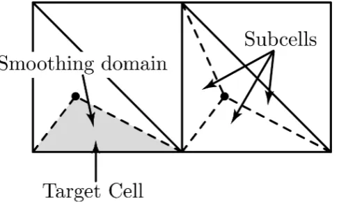
In this section, the basic idea behind cell-based-smoothed strain finite element method (CS-FEM) 52
element cell and numerical integration. In CS-FEM, a finite element is divided into three sub-cells that 54
called a smoothing domain as shown in Figure1. Over the smoothing domain, the strain-displacement 55
and the stiffness matrices are constructed, viz. strains and stresses are smoothed on smoothing domain, 56
and not on an element. 57
Figure 1.The subdivision of a finite element cell into sub-cells and construction of smoothing domain in CS-FEM.
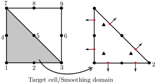
Another distinguished feature is the numerical integration. In strain-smoothing approach, the 58
numerical integration performs on the boundaries of smoothing domains as the line integration while 59
it performs in the element in FEM. Note that since the numerical integration is performed globally in 60
the proposed method, the Jacobian matrix is not required. To compute the strain-displacement matrix, 61
one Gauss point on the middle of the boundary of smoothing domain and outward normal vectors 62
are used. Figure2illustrates the integration scheme in CS-FEM with the location of Gauss points and 63
outward normal vectors. 64
Figure 2. The numerical integration of the strain smoothing method. Sub-cell412C is smoothing domain of CS-FEM. White square C is a centroid of the element and black circles are element nodes. Red circles are Gauss points located on the mid-point of the boundary of smoothing domain. Black arrows are the outward normal vectors at Gauss points.
For the nonlinear CS-FEM approximation, the following smoothed infinitesimal strain tensor over 65
∀x∈Ωsk, ε¯h(xk) =
Z
Ωs k
εh(x)Φ(x)dΩ, (1)
where a pointxkis located in smoothing domain andΦ(x)is the weight function. Using the divergence 67
theorem, the smoothed strain can be rewritten as: 68
¯
εh= 1
Ask
Z
Ωs k
εh(x)dΩ= 1
Ask
Z
Γs k
n(x)uh(x)dΓ, (2)
where Ask is the area of smoothing domain,Γskis the boundary of smoothing domain and n is the 69
outward normal vector in the form of the following matrix in two dimensions: 70
n(x) =
n1 0
0 n2
n2 n1
. (3)
The details of the method are given by Lee [15]. However, brief information of the smoothed 71
Galerkin weak form and its linearization is given as follows: 72
Z
Ω
∂W
∂F¯ (X, ¯F(u)):∇vdΩ=
Z
Ωf·vdΓ+
Z
ΓN
g·vdΓ, (4)
wherevis the set of admissible test function andFis the smoothed deformation gradient evaluated 73
over each smoothing domain. Equation (4) can be expressed with the energy functionR(u)and its 74
directional derivativesDR(u)·u: 75
R(u) =
Z
Ω
∂W ∂F¯ij
(X, ¯F(u)) ∂vi ∂XjdΩ
−
Z
Ω fividΩ+
Z
ΓN
gividΓ, (5)
DR(u)·u=
Z
Ω
∂2W ∂F¯ij∂F¯kl
(X, ¯F(u)) ∂vi ∂Xj
dΩ, (6)
wherei,j,k,l∈ {1, 2}for tow dimension andWis the stored strain energy function. 76
To find an approximate solution to Equation (4), the Newton-Raphson iterative method is 77
employed. At iteration iter+1, knowing the displacementuiter from iteration iter, findriter that
78
satisfies: 79
DR(uiter)·riter=−R(uiter). (7)
R(u) =
Z
Ω2
∂W ∂C¯ij
¯
Fki ∂vk ∂Xj
dΩ−
Z
Ω fividΩ+
Z
ΓN
gividΓ, (8)
and 81
DR(u)·r=
Z
Ω
∂2W ∂C¯ij∂C¯kl
¯ Fpi
∂vp ∂Xj
¯ Fsk
∂vs ∂Xl
+2∂W
∂C¯ij ∂rk ∂Xi
∂vk ∂Xj
!
dΩ, (9)
where ¯Cis the smoothed right Cauchy-Green deformation ¯C=F¯TF¯. 82
The global system of equations at each iteration can be written as: 83
¯
Kiterriter=b¯iter, (10)
thus, the displacementuis obtained by the iteration method: ¯uiter+1=u¯iter+riter.
84
2.2. Linear smoothing function in the framework of CS-FEM approximation 85
In the conventional strain smoothing method, the smoothing function f is a constant, that isf(x) = 86
1. This smoothing function is suitable for the strain smoothing approach with linear quadrilateral or 87
triangular elements. However, when the quadratic elements are used in S-FEM, the given smoothing 88
function cannot be used (Francis et al. [13]). Therefore, to use quadratic elements, the following linear 89
polynomial basis is chosen as the linear smoothing function: 90
f(x) =
0 x1 x2
, (11)
and its derivative is f,j(x) =
0 δ1j δ2j
T . 91
The right hand side of Equation (1) with the smoothing function would yield the basis function 92
derivatives level, which can be expressed as follows: 93
Z
Ωs k
Ψa,jf(x)dΩ=
Z
Γs k
Ψaf(x)njdΓ−
Z
Ωs k
Ψaf,j(x)dΩ, (12)
whereΨis the set of the shape functions. Note that in this work, Lagrange basis functions are used as 94
shape functions. For two dimensional problems, Equation (12) with the linear smoothing function (see 95
Z
Ωs k
Ψa,1f(x)dΩ=
Z
Γs k
Ψan1dΓ
Z
Ωs k
Ψa,1x1dΩ=
Z
Γs k
Ψax1n1dΓ− Z
Ωs k
ΨadΩ
Z
Ωs k
Ψa,1x2dΩ=
Z
Γs k
Ψax2n1dΓ,
(13)
and 97
Z
Ωs k
Ψa,2f(x)dΩ=
Z
Γs k
Ψan2dΓ
Z
Ωs k
Ψa,2x1dΩ=
Z
Γs k
Ψax1n2dΓ
Z
Ωs k
Ψa,2x2dΩ=
Z
Γs k
Ψax2n2dΓ− Z
Ωs k
ΨadΩ,
(14)
forΨa,1andΨa,2, respectively.
98
The cell-based smoothing domains are also used for the numerical integration for Equations (13) 99
and (14). Figure3shows the numerical integration scheme for the proposed cell-based strain-smoothed 100
method. In the proposed method, the finite element cell does not require to be divided into sub-cells 101
as the conventional CS-FEM. Namely, the finite element cell is the target cell and smoothing domain in 102
this case. 103
Figure 3.The construction of smoothing domain and numerical scheme in CS-FEM with the linear smoothing function for the quadratic triangular mesh. The interior Gauss points are black triangles while Gauss points on the boundaries are red circles. The outward normal vectors are depicted as black arrows.
Another feature that can be found in Figure3is the number of Gauss points. The proposed scheme 104
has two different Gauss point locations: first location can be found on the boundaries of smoothing 105
on the boundaries are required to compute for the smoothed stiffness matrix. Therefore, the following 107
system of equations is applied to evaluate the smoothed strain-displacement matrix: 108
Wdj= fj, j∈ {1, 2}, (15)
where 109 W=
1W 2W 3W 1W1x
1 2W2x1 3W3x1 1W1x
2 2W2x2 3W3x2
, (16)
f1=
3 ∑ k=1
2
∑ g=1Ψa
g
ks
kn1
g kv
3
∑ k=1
3
∑ g=1
Ψa
g
ks
g
ks1kn1gkv− 3
∑ m=1
Ψa(mr)mw
3
∑ k=1
2
∑ g=1
Ψa
g
ks
g
ks2kn1 g kv
f2=
3 ∑ k=1
2
∑ g=1Ψa
g
ks
kn2gkv
3
∑ k=1
3
∑ g=1Ψa
g
ks
g
ks1kn2gkv 3
∑ k=1
2
∑ g=1
Ψa
g
ks
g
ks2kn2gkv− 3
∑ m=1
Ψa(mr)mw
, (17) and 110
dj =
1d
j 2dj 3dj
T
=
Ψa,j 1r
Ψa,j 2r
Ψa,j 3r
T
. (18)
The coordinates of themthinterior Gauss points are defined asmr= (mr1,mr2)and their weights
111
are given asmw. On the other hand, the coordinates ofgthGauss pointsgks = gks1,kgs2
and their 112
weights gkvare given at the kth boundaries of smoothing domain. The outward normal at thekth 113
boundary of smoothing domain is given askn= (kn1,kn2). Equation (18) denotes the solution vector
114
of Equation (15). Thejth basis function derivatives are obtained at the three interior Gauss points
115
in each smoothing domain (Figure3). Using the obtained solution vector, the modified smoothed 116
strain-displacement matrix can be obtained: 117
¯
Bkr=
¯ B1
kr B¯
2
kr · · · B¯ n
kr
, k∈ {1, 2, 3}, (19)
¯ Ba
k
r=
kd
1 0
0 kd2
kd
2 kd1
. (20)
3. Results
119
In this section, the validity and stability of the proposed linear smoothing function for the 120
quadratic triangular elements in nonlinear problems are demonstrated. The following series of 121
benchmark tests are studied: 1) simple shear deformation with Dirichlet and mixed Dirichlet and 122
Neumann boundary conditions (BCs), 2) uniform extension with lateral contraction with Dirichlet and 123
mixed Dirichlet and Neumann BCs, 3) “Not-so-simple” shear deformation with Dirichlet BCs and 4) 124
bending of a rectangular block with Dirichlet BCs. 125
For nonlinearity, a neo-Hookean hyperelastic model is used [16]: 126
W= 1
2(lnJ)
2−
µlnJ+1
2µ(trC−3), (21)
where Lamé’s first parameterλ=κ−(1/2)µis defined using the shear modulusµand bulk modulus 127
κin two dimensions. The Jacobian is given asJ=detF. The present CS-FEM is compared with the exact 128
solutions and quadratic triangular elements in FEM. The details of numerical tests, i.e. implementation 129
of boundary conditions and exact solutions in strain energy can be found in References [6] and [15]. 130
Note that benchmark tests are considered as the dimensionless. 131
3.1. Discussion 132
3.1.1. Simple shear deformation 133
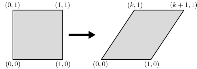
First, simple shear deformation with two different types of boundary conditions are considered: 134
1) Dirichet BCs and 2) mixed Dirichlet and Neumann BCs. Figure4depicts the initial and deformed 135
shapes of the unit square for the problem. 136
To impose Dirichlet and Neumann BCs for simple shear deformation, the following deformation 137
gradient and first Piola-Kirchhoff stress tensor are defined, respectively: 138
F=
1 k 0 0 1 0
0 0 1
, (22)
and 139
P=
0 kµ 0
kµ 0 0
0 0 0
, (23)
wherek>0 and its strain energy using Equation (21) is given as: 140
W= µ
2k
2. (24)
The present work usesk= 1 for the deformation gradient. To compute the strain energy, the 141
shear modulusµ=0.6 and bulk modulusκ =100 are used, which is equivalent to Poisson’s ratio 142
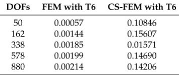
ν=0.497. Hence, the strain energy for simple shear deformation is determined to be W=0.3. Tables1 143
and2provide the detailed values of displacement relative error for FEM and proposed CS-FEM with 144
the quadratic 6-node node triangular (T6) element. It can be found that the proposed method shows 145
the exact solution down to machine precision. 146
Table 1.Displacement relative error (×10−12) for simple shear deformation with Dirichlet BCs.
DOFs FEM with T6 CS-FEM with T6
50 0.00057 0.10846
162 0.00144 0.15607
338 0.00185 0.01571
578 0.00199 0.14690
880 0.00214 0.14206
Table 2. Displacement relative error (×10−12) for simple shear deformation with Dirichlet and Neumann BCs.
DOFs FEM with T6 CS-FEM with T6
50 0.10186 0.13922
162 0.10172 0.14249
338 0.10038 0.13953
578 0.09941 0.13973
3.1.2. Uniform extension with lateral contraction 147
The next test is uniform extension with lateral contraction using Dirichlet and mixed Dirichlet 148
and Neumann BCs. The geometry and material properties used are the same as the simple shear 149
deformation. The deformation gradient and non-zero components of the first Piola-Kirchhoff stress 150
tensor are: 151
F=
λ1 0 0
0 λ2 0
0 0 λ2
, (25)
and 152
P11 =
σ11
λ1
=µ
λ1−
1
λ1
=−P22, (26)
whereλ1 =1.15,λ2 =1/λ1andλ3 =1. HenceP11 = −P22 =0.16826087 and the strain energy is
153
W= µ2
λ21+ 1 λ21 −2
≈0.02359. 154
Figures5and6illustrate the deformed shapes of uniform extension with lateral contraction using 155
Dirichlet and mixed Dirichlet and Neumann BCs, respectively. Figure7shows the convergence of the 156
displacement relative errors of FEM and proposed CS-FEM with linear smoothing for the problem 157
with Dirichlet and mixed Dirichlet and Neumann BCs. As shown in Figure7, a fraction is within 158
machine precision with portion 10−14for FEM and 10−12for the present method.
159
Figure 6.Deformed shapes of uniform extension with lateral contraction with mixed Dirichlet and Neumann BCs: (a) FEM with T6. (b) the proposed CS-FEM with T6.
Figure 7.Convergence of the displacement relative errors of FEM and CS-FEM for uniform extension with lateral contraction with Dirichlet and mixed Dirichlet and Neumann BCs.
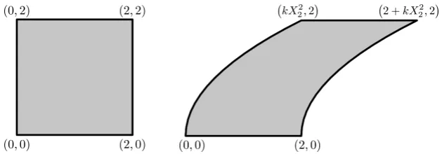
3.1.3. “Not-so-simple” shear deformation 160
This test is a non-homogeneous deformation example known as “Not-so-simple” shear 161
deformation with Dirichlet BCs. As shown in Figure8, the geometry of this problem is(0, 2)×(0, 2) 162
and its deformation gradient is given in Equation (27). 163
F=
1 2kX2 0
0 1 0
0 0 1
, (27)
wherek>1. The exact solution in strain energy is given as W= µ
2(2kX2)2=2µk2X22=1.6 since the 164
shear and bulk moduli are the same as simple shear deformation. 165
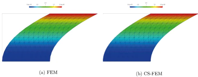
Figure9depicts the deformed shapes of “Not-so-simple” shear deformation with Dirichlet BCs 166
for FEM and the proposed scheme. 167
Figure 9.Current configuration of “Not-so-simple” shear deformation with Dirichlet BCs: (a) FEM with T6. (b) proposed CS-FEM with T6.
As given in Figure10a, the displacement error for FEM and proposed CS-FEM is almost identical. 168
The convergence of relative error in strain energy is given in Figure10b. In this case, the present 169
method is more accurate than FEM. 170
Figure 10. Convergence of displacements and strain energy relative errors: (a) relative error in displacements. (b) relative error in strain energy given as Wrelative error=Wnumerical/Wexact.
3.1.4. Bending of a rectangular block 171
Lastly, an additional non-homogeneous deformation such as bending of a rectangular block is 172
investigated. For this problem, shear modulusµ = 0.6 and bulk modulusκ = 1.95 equivalent to 173
Figure 11.The geometry of the rectangular block for bending test. In this work, the length on x-axis A=2,A=3 and length on y-axisB=2 are used.
For the implementation of Dirichlet BCs, the following cylindrical coordinates in Cartesian 175
coordinates are defined: 176
x=rcosθ= √
2αXcosY α
y=rsinθ= √
2αXsinY α
z=0,
(28)
where(x,y,z)are the current Cartesian coordinates and(X,Y,Z)are the initial Cartesian coordinates. 177
Thus the deformation gradient for this test can be obtained as: 178
F=
f0(X) 0 0
0 f(x)g0(Y) 0
0 0 1
, (29)
where f(X),g(Y),f0(X)andg0(Y)are: 179
f(X) =√2αX
f0(X) = √
2α
2√X g(Y) = 1
αY
g0(Y) = 1 α,
(30)
where the bending factorα=0.9 is used for this work. Hence, the exact strain energy can be computed 180
W=
Z 3 2
Z 2
−2
(
µ(0.9−2X)
2
3.6X )
dV≈4.485618. (31)
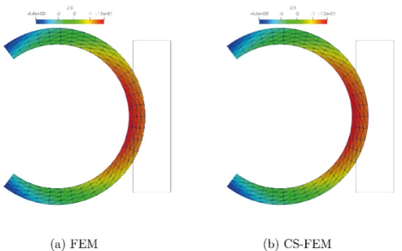
Figure12illustrates the deformed shapes of the present example for FEM and proposed linear 182
smoothing function scheme. In this study, two cases categorized by different of numbers of elements 183
along each side are used: 1) case 1 is 2×4, 2×8, 2×12, 2×16, 2×20, 2×24, 2×28, 2×32 and 2) 184
case 2 is 4×4, 4×8, 4×12, 4×16, 4×20, 4×24, 4×28, 4×32. When the bending factorαis bigger, 185
the deformed shape becomes a circle as shown in Figure12. 186
Figure 12. Deformed shapes of the rectangular block for bending problem: (a) FEM with T6. (b) CS-FEM with T6.
Figure13provides the convergence of displacements and strain energy relative errors in two 187
cases. For both FEM and CS-FEM, relative errors in displacements are almost the same in two cases 188
as shown in Figure13a. However, the strain energy relative error for the proposed method in two 189
different cases is identical and more accurate than FEM. 190
4. Conclusions
191
In this paper, the linear smoothing function is employed to the cell-based strain-smoothed finite 192
element approximation for the problem of two-dimensional nonlinear hyperelasticity. Unlike the 193
conventional S-FEM, the proposed scheme does not require to the division of finite element cells into 194
sub-cells. Namely, the quadratic triangular element used the smoothing domain itself. Moreover, no 195
further intervention for subdivision is required. Hence, this leads to an increase in the implementation 196
efficiency for the proposed method code. The present CS-FEM with the linear smoothing scheme 197
needs two Gauss points on the boundaries of smoothing domains and three interior Gauss points in 198
the domain. The smoothed strain-displacement matrix is evaluated at the interior Gauss points. 199
The present CS-FEM is examined by a series of numerical tests to validate its accuracy and 200
stability. The obtained results are compared with the exact solutions. From the results carried out 201
in numerical tests, the following conclusions are obtained: 1) in the homogeneous deformation 202
problem, the proposed CS-FEM with the linear smoothing scheme is able to reproduce machine 203
precision in displacement relative error that is identical to the strain energy relative error and 2) in 204
the non-homogeneous deformation problem, the present scheme shows more accurate results than 205
FEM with fast convergence rate to the exact solution. In future work, the proposed linear smoothing 206
functions to edge-based and node-based strain smoothing approximation will be employed which 207
would effectively handle locking and are less sensitive to distorted meshes than the CS-FEM. 208
Author Contributions:Conceptualization, C.L. and S.N.; methodology, C.L. and S.N.; software, C.L.; validation, 209
C.L. and S.N.; formal analysis, C.L.; writing–original draft preparation, C.L.; writing–review and editing, S.N.; 210
visualization, C.L.; supervision, S.N.; funding acquisition, C.L. 211
Funding: This research was funded by National Research Foundation (NRF) of Korea through Ministry of 212
Education under the grant number No. 2016R1A6A1A03012812. 213
Conflicts of Interest:The authors declare no conflict of interest. 214
References
215
1. Liu, G.R.; Dai, K.Y.; Nguyen, T.T. A smoothed finite element method for mechanics problems.Computational 216
Mechanics2007,39(6), 859–877. 217
2. Liu, G.R.; Nguyen, T.T.; Dia, K.Y.; Lam, K.Y. Theoretical aspects of the smoothed finite element method 218
(SFEM).International Journal for Numerical Methods in Engineering2007,71(8), 902–930. 219
3. Liu, G.R., Nguyen, T.T.Smoothed Finite Element Methods, CRC Press: Boca Laton, Florida, USA; 2010. 220
4. Nguyen-Xuan, H.; Rabczuk, T.; Bordas, S.; Debongnie, J.; A smoothed finite element method for plate 221
analysis.Computer Methods in Applied Mechanics and Engineering2008,74, 175–208. 222
5. Nguyen-Thanh, N.; Rabczuk, T.; Nugyen-Xuan, H.; Bordas, S.P. A smoothed finite element method for shell 223
analysis.Computer Methods in Applied Mechanics and Engineering2008,198, 165–177. 224
6. Lee, C.K.; Angela Mihai, L.; Hale, J.S.; Kerfriden, P.; Bordas, S.P.A. Strain smoothing for compressible and 225
7. Ong, T.H.; Heaney, C.E.; Lee, C.K.; Liu, G.R.; Nguyen-Xuan, H. On stability, convergence and accuracy 227
of bES-FEM and bFS-FEM for nearly incompressible elasticity.Computer Methods in Applied Mechanics and 228
Engineering2014,285, 315–345. 229
8. Bordas, S.; Natajaran, S.; Kerfriden, P.; Augarde, C.; Mahapatra, D.; Rabczuk, T.; Pont, T. On the performance 230
of strain smoothing for quadratic and enriched finite element approximations (XFEM/GFEM/PUFEM). 231
International Journal for Numerical Methods in Engineering,2011,86, 673–666. 232
9. Bordas, S.P.; Rabczuk, T.; Nguyen-Xuan, H.; Nguyen, V.P.; Natarajan, S.; Bog, T.; Quan, D.M.; Hiep, N.V. 233
Strain smoothing in FEM and XFEM.Computational & Structures2010,88, 1419–1443. 234
10. Jiang, C.; Zhang, Z.Q.; Han, X.; Liu, G.R. Selective smoothed finite element methods for extremely 235
large deformation of anisotropic incompressible bio-tissues. International Journal for Numerical Methods 236
in Engineering2014,99(8), 587–610. 237
11. Natarajan, S.; Bordas, S.P.A.; Ooi, E.T. Virtual and smoothed finite elements: a connection and its application 238
to polygonal/polyhedral finite element method.International Journal for Numerical Methods in Engineering 239
2015,104, 1173–1199. 240
12. Natarajan, S.; Ooi, E.T.; Chiong, I.; Song, C. Convergence and accuracy of displacement based finite element 241
formulation over arbitrary polygons: Laplace interpolants, strain smoothing and scaled boundary polygon 242
formulations.Finite Elements in Analysis and Design2014,85, 101–122. 243
13. Francis, A.; Ortiz-Bernardin, A.; Bordas, S.P.A.; Natarajan, S. Linear smoothed polygonal and polyhedral 244
finite elements.International Journal for Numerical Methods in Engineering2017,109, 1263–1288. 245
14. Rand, A.; Gillette, A.; Bajaj, C. Quadratic serendipity finite elements on polygons using generalized 246
barycentric coordinates.Mechanics of Computations2014,83, 2691–2716. 247
15. Lee, C.K. Gradient smoothing in finite elasticity: near-incompressibility. PhD, Cardiff University, Cardiff, 248
Wales, UK, 2015. 249
16. Belytschko, T.; Moran, B.; Liu, W.K.Nonlinear Finite Element for Continua and Structures; John Wiley & Sons 250