Visualization and evaluation of flow during water filtration: Parameterization and sensitivity analysis

a

Corresponding author: [email protected]

Visualization and evaluation of flow during water filtration:

Parameterization and sensitivity analysis

Petr Bílek1,a

1

Technical University of Liberec, Studentská 1402/2, 461 17, Liberec 1, Czech Republic

Abstract. This paper deals with visualization and evaluation of flow during filtration of water seeded by artificial microscopic particles. Planar laser induced fluorescence (PLIF) is a wide spread method for visualization and non-invasive characterization of flow. However the method uses fluorescent dyes or fluorescent particles in special cases. In this article the flow is seeded by non-fluorescent monodisperse polystyrene particles with the diameter smaller than one micrometer. The monodisperse sub-micron particles are very suitable for testing of textile filtration materials. Nevertheless non-fluorescent particles are not useful for PLIF method. A water filtration setup with an optical access to the place, were a tested filter is mounted, was built and used for the experiments. Concentration of particles in front of and behind the tested filter in a laser light sheet measured is and the local filtration efficiency expressed is. The article describes further progress in the measurement. It was carried out sensitivity analysis, parameterization and performance of the method during several simulations and experiments.

1 Introduction

Visualization and evaluation of flow is a suitable tool for investigation of flow, verification of numerical data and measurement of flow parameters. Various experimental methods were developed to measure important parameters of flow in different conditions. The most wide spread visualization and measuring methods are PLIF (planar laser induced fluorescence), PIV (particle image velocimetry), IPI (interferometric particle imagining) and shadow sizing [1, 2]. Even though the methods exist in many variants they have not to be suitable in some specials cases of use.

In this article the visualization of flow enables to see the filtration process in a laser sheet by a digital camera. This optical method helps to see, what is happening inside a filtration chamber and enables to measure the local filtration efficiency. The water filtration setup with an optical access is used for the experiments. Water is seeded by artificial submicron particles and the suspension is filtered by a tested filtration textile. In this article monodisperse non-fluorescent polystyrene particles with its diameter below one micron are used. The captured digital images of the filtration process are analysed and the local filtration efficiency is expressed. The measuring method is a relative method and it measures on the basis of a calibration. The calibration is carried out by known mass concentration of polystyrene particles. The most important issue is to keep the same conditions during the calibration and then during the

measurement. More about the first experiments using PLIV and PIV method is in [3].

In this paper the new progress of the measuring method is discussed. The impact of a change of particle size, angle between the camera and the laser sheet, size of an evaluative area and flow velocity to the measurement were monitored. Also parameters of the method in various setting of the camera and the filtration setup were expressed.

2 Experimental setup

The filtration process is investigated in the filtration channel, where an optical access is enabled. The filtration channel is connected to the water filtration circuit, where two pressure sensors, a flow meter and a pump are mounted, Figure 1. In this article the water filtration setup is used only for the determination of the impact of flow velocity on measured results.

Due to the simplification of the other experiments a glass tank was used instead of the filtration chamber including the whole filtration setup. The glass tank was made from the same material as the filtration chamber, where a tested filter mounted is, so the optical parameters are the same. The picture of the setup with the glass container is shown in Figure 2. The glass container is usually used for calibration of the filtration channel. In this paper the glass tank is used for the sensitivity analysis.

C

Owned by the authors, published byEDP Sciences, 2016

The flow is illuminated by the laser sheet generated by a 10° wobble angle Powell lens and a laser module. The laser module generates a 1 mm narrow green laser beam with the power of 92.8 mW (measured by LabMaster Ultima v. 2.35 with an attenuator 1:1000).

Figure 1. Scheme of the water filtration setup with the filtration channel and the laser sheet. The camera is installed at the place of a viewer.

Figure 2. Picture of the setup with the glass tank instead of the filtration chamber including the filtration setup.

The laser sheet is show in Figure 3. Unfortunately the laser sheet is not uniform and it includes brighter and darker strips about different light intensities. This is caused by defects of the cylindrical lens as well as the laser beam. The curve of a digital grey value across the laser sheet is shown in the graph in Figure 4. We can see the very uneven irradiation of the flow in the laser sheet. Nevertheless the defects of the laser sheet can be corrected by the calibration during evaluation of the filtration process. The camera is Pike F-210B/C with 1 inch size CCD chip with resolution 1920 × 1080 pixels.

The camera offers plenty of settings and it is equipped by Samyang 35 mm F1.4 lens. The seeded particles are monodisperse made of polystyrene. The particles have excellent optical and mechanical features. The used sizes are 0.28, 0.42, 0.69, 0.96 and 1.7 micrometers.

Figure 3. The laser sheet in the glass tank full of water seeded by 0.69 μm polystyrene particles.

Figure 4. Graph of the digital grey value across the laser sheet, created by ImageJ software [4].

3 Experimental

The optical method for an evaluation of the local filtration efficiency is a relative method based on a calibration. The measuring conditions during the calibration have to be the same as during the measurement. In this article the impact of change of some chosen parameters between the calibration and the measurement was investigated. The parameters are scattering angle (the camera elevation against the laser sheet), particle size, flow rate and size of an evaluative area (the investigative area in an image, where the local concentration calculated is).

A part of the sensitivity analysis was carried out on the basis of simulations of the light scattering by small particles. A light intensity of the scattered light by small particles

ሺߠሻ ൌ ܧ଴ή஼ή௏ήȁௌሺఏሻȁ మ ௞మ_ήௗ

భమ ቂ ୛

୫మቃ (1)

is directly proportional to the scattering function |S()|2

an incident light intensity, V is a small volume (characterized by the size of an evaluative area and the thickness of a laser sheet), is scattering angle, k is wave number and d1 is the distance between an observer and particles [5]. In Figure 5, we can see the scattering function versus scattering angle for different sizes of particles. The scattering diagrams were created according to the Mie theory in software MiePlot [6]. The scattering diagrams were created for the used laser light and polystyrene particles suspended in distilled water.

Figure 5. Scattering diagrams for polystyrene particles, generated by MiePlot [6].

According to (1) the change of a measured concentration value copies the change of a scattering function. Method sensitivity to the variation in a scattering angle is expressed by

ܵఏൌ

ȁಷሺవబǤఱιሻషಷሺఴవǤఱιሻȁ ಷሺవబιሻ ήଵ଴଴

௱ఏ ቂ

Ψ

ιቃǡ (2)

where F is the scattering function and it is equal to |S()|2

and = 90.5 – 89.5 = 1° is a small change of the scattering angle around the right angle. The scattering angle is the angle between a laser sheet and a camera and its value is usually right angle = 90°. The scattering angle is in fact the angle represeting a camera elevation against the laser sheet. The functions F were calculated by the MiePlot software.

Method sensitivity to the variation in a particle size is expressed by

ܵ]ൌ

ȁಷሺ]శయΨሻషಷሺ]షయΨሻȁ ಷሺ]ሻ

೩] ]

ሾെሿǡ (3)

where Ø is size of a particle and Ø is the small change 6 % from the nominal value Ø. The functions F were also calculated by the MiePlot software.

Method sensitivity to the variation in a flow rate is determined on the basis of an expeirment. The experiement was carried out on the water filtration setup. Water in rezervoir was seeded artificial particles and the flow through the filtration chamber was step by step increased from zero to 20 liter per minute. For every flowrate ten pictures of the flow were taken. The shift of particles in an image

݀௧௘ൌ _஺ொ_ೌ೛ೡή௧_ή௓೐ ൏ ݀௣, (4)

should be smaller than the size of an active pixel dp, where Qv is volumetric flow rate, te is shutter time, Aap is cross section of the filtration channel and Z is zoom of an objective. Relative error is calculated according to

ߜ ൌு೘ିுೞ

ுೞ ൉ ͳͲͲሾΨሿǡ (5)

where Hm is a measured value obtained from the measurement and Hs is the real value (calculated from the first 5 measurements during very low flowrate). The values can be expressed as digital grey values.

Method sensitivity to the variation in the size of an evaluative area is determined by another experiment, which was carried out with a glass tank instead of the filtration chamber and whole filtration setup. The concentration of artificial seeding particles was prepared to 100 μg per litre. The laser sheet was aimed to the glass tank and it was captured by the digital camera. Ten pictures were made. From these ten pictures a variation coefficient was calculated for the different sizes of an evaluative area and the different sizes of particles. The variation coefficient is expressed according to

ܥ௩ൌఙ_஼തതതതത಴೘_೘ሾΨሿǡ (6)

where Cm is a standard deviation and ܥ௠തതതത is an average value of a mass cocnetration.

The last experiment was carried out with the glass tank as well. The concentration of artificial seeding particles was increased step by step in the glass tank and for every step ten pictures were taken. The concentration was increased from zero to 20 mg per liter. The calibration constant and the method sensitivity were calculated for various sizes of polystyrene particles. The sensitivity of the measuring method

ܵ஼௠ൌ_୼஼୼௒_೘೛ ൌ_௄ଵ_೅ቂୢ୫ య

ஜ୥ ቃ (7)

is calculated from the change of the digital gray value

Yp and the change of the mass concentration Cm. The smallest digital grey value is one, so the sensitivity is equal to the reciprocal calibration constant KT.

4 Results

4.1 Sensitivity analysis

4.1.1 Angle between the camera and the laser sheet

Nevertheless the sensitivity for the large particles is much smaller, if they are polydisperse. In fact no particles are absolute monodisperse and the majority of offered monodisperse particles are in fact polydisperse particles with a standard deviation. This implies that for the large particles the sensitivity is not such high.

Table 1. Method sensitivity to the scattering angle.

Particle size

Ø [μm] 0.1 0.28 0.42 0.69 0.96 1.7 10

S [% / °]

Monodisperse particles

0.5 7.5 4 4.9 4.1 6.3 120

S [% / °]

Polydisperze, Std. Dev. 2 %

0.54 7.48 3.88 4.51 3.33 2.95 6.71

4.1.2 Size of seeding particles

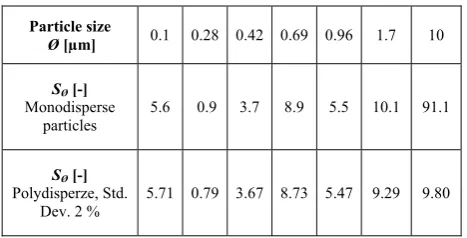
The sensitivity of the optical method to particle size was calculated according to (3) and it is shown in Table 2. The particle size can be changed by dissolving or swelling of particles in water. The change of its size can cause significant error in measurement. For monodisperse particles the sensitivity is again higher for bigger particles. It is caused by its vibrating scattering diagram. In fact the sensitivity is much smaller due to standard deviation in size of the standard supplied particles.

Table 2. Method sensitivity to the size of seeding particles.

Particle size

Ø [μm] 0.1 0.28 0.42 0.69 0.96 1.7 10

SØ [-]

Monodisperse particles

5.6 0.9 3.7 8.9 5.5 10.1 91.1

SØ [-]

Polydisperze, Std.

Dev. 2 % 5.71 0.79 3.67 8.73 5.47 9.29 9.80

4.1.3 Flow rate in the filtration chamber

The optical method works during the wide range of flow rates. In Figure 6 we can see the influence of a relative error of the concentration measurement to the volumetric flow rate. The relative error was calculated according to (5).

Figure 6. Graph of a relative error versus volumetric flow rate.

In the graph there are three curves for three exposition times. The relative error is the highest for the longest exposition time. This is caused by a blurring of an image according to (4). If the volumetric flow rate is high, the velocity of the particles in the filtration channel is high as well and the higher concentration of particles is measured in the blurred picture. The orange curve in the graph increases, though it is obtained during a very low shutter time. This is caused by air bubbles. The air bubbles are new sources of a scattered light and the method measures it as a higher mass concentration. In fact the mass concentration is still the same.

4.1.4 Size of the evaluative area

The graph in Figure 6 shows us the influence of the size of an evaluative area in an image. The variation coefficient was calculated according to (6). We can see high values for bigger particles. This is caused by distinguishability of the seeding particles in an image. In general the variation coefficient is the higher, the evaluative area is smaller.

Figure 7. Graph of the variation coefficient versus size of an evaluative area.

4.2 Parameterization

The Table 3 shows the calibration constants and sensitivities of the optical method according to the used

-5 0 5 10 15 20 25 30 35

0 5 10 15

Relative error

/

%

Volumetric flowrate Qv/ liter per min

te = 20 ms te = 2 ms te = 0.2 ms

0 5 10 15 20 25 30 35 40 45 50

1 10 100

Variation coefficient

Cv

/

%

Size of an evaluative area O_x/ px

polystyrene particles. The sensitivity was calculated according to (7). We can see that the method is the most sensitive for the smallest particles. This is caused by their high number during the same mass concentration.

Table 3. Calibration constants for different particle sizes.

Particle size KT [μg/ dm3_{] S}

Cm [dm3_{/g] Range[μg/dm}3_]

0.28 μm 0.03897 26 0.04 - 2620

0.42 μm 0.06104 17 0.06 - 3932

0.69 μm 0.07484 13 0.08 - 5242

0.96 μm 0.08098 12 0.08 - 5242

1.7 μm 0.10841 10 0.1 - 6553

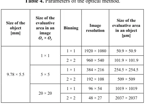
The range of the measured mass concentration varies according to the sensitivity. Therefore the dynamic rage of the camera is still the same. The range of the optical method can be changed by setting of the camera, Table 4. If the binning is activated, the sensitivity is higher, but resolution is lower. If the evaluative area is bigger, the resolution of the method decreases. It is all about compromises and the optical method can be more powerful only in case of a better camera or a higher power of the laser sheet.

Table 4. Parameters of the optical method.

Size of the object [mm]

Size of the evaluative area in an image

Ox × Oy

Binning Image

resolution

Size of the evaluative area

in an object [μm]

9.78 × 5.5

1 × 1

1 × 1 1920 × 1080 50.9 × 50.9

2 × 2 960 × 540 101.9 × 101.9

5 × 5

1 × 1 384 × 216 254.5 × 254.5

2 × 2 192 × 108 509 × 509

20 × 20

1 × 1 96 × 54 1019 × 1019

2 × 2 48 × 27 2037 × 2037

5 Conclusion

The optical method for an evaluation of a filtration process discussed in the article is a strong tool for achievement new information about a filter. The method enables to visualize flow in the vicinity of the filter and characterize the filtration process. It is possible to measure the local filtration efficiency, which is connected to the geometrical structure of a filter. In this article a sensitivity analysis and a parameterization were carried out. Some of the measurements were simplified by a glass tank with the same optical performance as the filtration chamber. The glass tank was used instead of the filtration channel and water inside was seeded by polystyrene monodisperse particles.

The performance of the method is influenced by type of used particles, power of the laser module and settings of the digital camera. In general the method is capable to detect particles in range of 0.1 to 100 μm. The particles bigger than hundred of microns can be detected as well,

but there is no requirement to measure these large particles. Smaller particles are detectable only in case of change of the camera setting to the most sensitivity mode at the expense of lower resolution or higher relative error. The small particles have to be in higher mass concentration as well. The maximum acceptable flow rate can be around 5 litres per minute for the used filtration chamber (5 cm). For higher values the relative error increases significantly because of blurring images and air bubbles occurring in the filtration chamber. The minimum size of an evaluative area in an image can be 10 × 10 pixels. The smaller values cause significant increase of a relative error. The method is very versatile and can measure wide range of particle sizes and their concentrations. However the versatility is limited by dynamic range of the digital camera. It is about compromises, the method can be very sensitive, but only in case of very low resolution and vice versa.

From the sensitivity analysis it ensures that the sensitivity of the optical method to the camera elevation (scattering angle) and size of particles is quite high. The calculations are propping upon Mie theory through the software MiePlot. The result is that the camera elevation against the laser sheet during the calibration has to be the same as during the measurement. To prevent size modification of seeding particles caused by swelling or dissolving, the particles have to be in water for the same time as during the calibration as during the measurement.

Acknowledgments

This work was supported by the Ministry of Education of the Czech Republic within the SGS project no. 21066/115 on the Technical University of Liberec.

References

1. C. Tropea, A. L. Yarin, J. F. Foss, Springer handbook of experimental fluid mechanics, Springer science and business media, p. 1557, ISBN: 978-3-540-25141-5, (2007).

2. J. E. Martin, M. H. García, Combined PIV/PLIF measurements of a steady density current front, Experimental fluids 45, p. 265-276, (2009).

3. D. Jašíková, M. Kotek, P. Šidlof, J. Hrza, M. Komárek, V. Kopecký : Nanofilter evaluation using visualization methods, 1st Nanocon International Conference, Tanger Ltd., pp. 186. (2009).

4. ImageJ. Image analysis software

[online: 22.5.2015].

URL: <http://rsbweb.nih.gov/ij/index.html>.

5. H. G. van de HULST, Light Scattering by Small Particles. Willey, New York, pp. 470, ISBN: 0-486-64228-3, (1957).