ABSTRACT
TETTEH, ISAAC KOW. Three-Dimensional Characterization of Boreal Spring-Summer Climate Variability over West Africa (1948-2006). (Under the direction of Dr. Fredrick H. M. Semazzi).
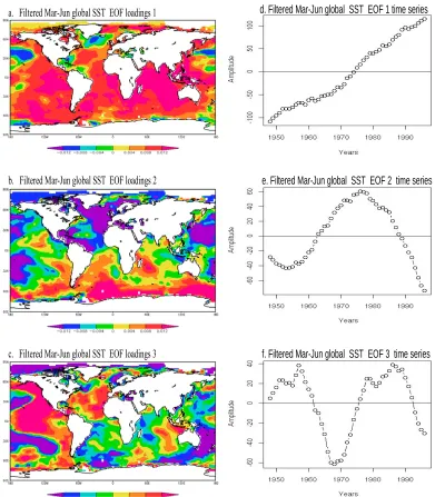
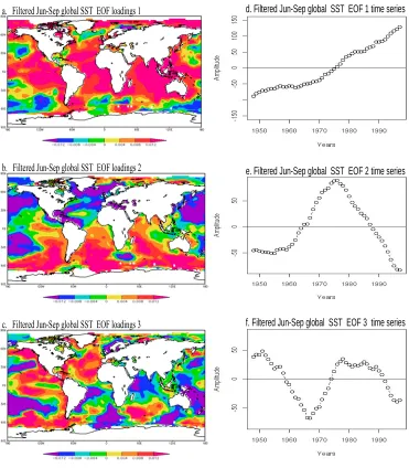
The main scientific interest is to characterize the three-dimensional boreal spring-summer climate anomaly patterns from 1948-2006 using monthly UD terrestrial precipitation, ERSST, and NCEP/NCAR reanalysis data for two major rainfall seasons, March-April-May-June (MAMJ) and June-July-August-September (JJAS) over tropical West Africa. The study is organized into two parts, which entail the use of: (i) unfiltered data for general characterization, and (ii) a 10-year low-pass-filtered data to focus on decadal/low frequency (LF) structures.
Velocity potential (divergence) and streamfunction (rotational) are computed from the horizontal wind fields. The linear regression model is used to evaluate the functional relationship between the net precipitation and net vertically integrated moisture budget (NVIMB) anomalies for the two seasons over West Africa, Sahel, and GOGC, and also, test the sensitivity of the divergent circulations over these climatic zones.
Three-Dimensional Characterization of Boreal Spring-Summer Climate Variability over West Africa (1948-2006)
by
Isaac Kow Tetteh
A thesis submitted to the Graduate Faculty of North Carolina State University
in partial fulfillment of the requirements for the degree of
Master of Science
Marine, Earth, and Atmospheric Sciences
Raleigh, North Carolina 8th July 2009
APPROVED BY:
_______________________________ ______________________________ Dr. Fredrick H. M. Semazzi Dr. Lian Xie
DEDICATION
BIOGRAPHY
Isaac Kow Tetteh, affectionately called Paa Kow, was born in Takorase in the Eastern Region of Ghana, to Mr. Albert Tetteh, of blessed memory, and Madam Faustina Sam. He started his primary education at Urban Council Primary and Middle School, in Winneba, Central Region, and completed his G.C.E Ordinary and Advanced Level education at Winneba Secondary School (WSS). He did his post-secondary school National Service at WSS. In 1985, he gained admission to the University of Cape Coast (UCC), where he obtained his BSc (Hon) Degree in Biological Sciences and a Diploma in Education in 1989. As a professional teacher, he taught Health Science, General Science, Integrated Science, and Biology at Accra Workers’ College, Accra Polytechnic, and Prempeh College, all in Ghana. In 1996, he gained admission to the Kwame University of Science and
Technology (KNUST), Kumasi, Ghana, where he obtained his MSc Degree in Environmental Science. He worked with the Department of Theoretical and Applied Biology, KNUST, until he was awarded Government of Ghana Scholarship to pursue graduate studies in
ACKNOWLEDGMENTS
“The mighty God omniscient one, whose ways we cannot trace. He reckons every good begun and crowns it with His grace. He is here and there and everywhere, in all the ways I have trodden. I have never passed beyond the sphere of the providence of God.” Thank you, God, the creator and sustainer of the universe, in whom all things consist, for bringing me to this stage in my career.
I am also, highly indebted to Dr. F. Semazzi, my advisor, for his guidance and devoting his time to mentor me to produce this piece of work. I will also thank my Thesis Advisory Committee members, Drs. L. Xie and A. Aiyyer, for their guidance and
constructive criticisms. Also, I acknowledge the various forms of assistance I gained from my peers of Climate Modeling Laboratory, especially, Neil Davis, Jared Bowden, Kara Smith, Matthew Norman, Sean Heuser, Robert Mera, and Michael Diaz. I am indeed very grateful for the support I continue to receive from my wife, Antonia, my children (Kweku, Esi, and Araba), my mother and siblings.
TABLE OF CONTENTS
LIST OF TABLES………...ix
LIST OF FIGURES………..x
CHAPTER ONE ………. ....1
1. Introduction ………1
1.1 Problem Identification and Significance of the Research ………...1
1.2 Objective(s) and Structure of the Thesis ………3
1. 2.1 Objective(s) of the Research ………3
1. 2. 2 Structure of the Thesis .………4
1.3 Literature Review ………..4
1.3.1 Techniques for Analyzing Multivariate Data in Climate Research……...4
1.3.2 Significance tests of principal components ……….6
1.3.3 Data Filtering Techniques ………..7
1.3.4 West African Climate variability and atmospheric circulation ………9
CHAPTER TWO ………...13
2. Data and Methods ………...13
2.1 Data Sources and Description ……….13
2.1.1 NCEP-NCAR Reanalysis 1 Data ………13
2.1.3 Sea surface temperature data ……….15
2.1.4 Teleconnection Indices .……….15
2.2 Methods ………...16
2.2.1 Analysis Domain and Time Scales ……….16
2.2.2 Analysis Techniques………16
2.2.2.1 EOF Analysis and Significance Test………...16
2.2.2.2 Construction of IOSSD Index ………...17
2.2.2.3 Correlation Analyses………..18
2.2.2.4 Composite Analyses ………..18
2.2.2.5 Velocity potential and streamfunction anomaly analysis………...19
2.2.2.6 Moisture budget anomaly analysis ………20
2.2.2.6.1 Atmospheric vapor budget anomaly analysis………...20
2.2.2.6.2 Regression model for the analysis of net precipitation and moisture budget anomalies………22
CHAPTER THREE………23
3. Results and Discussion: Generalized (unfiltered) Structures………...23
3.1 EOF Analysis and West African precipitation-global SST covariability………...23
3.1.1 MAMJ and JJAS West African precipitation variability………23
3.1.2 MAMJ and JJAS global SST variability……….30
3.1.3 MAMJ/JJAS West Africa rainfall and MAMJ/JJAS global SST relationships……….34
3.2.1 Unfiltered surface circulation mechanism………...42
3.2.2 Unfiltered atmospheric circulation anomalies at 850 hPa………...48
3.2.3 Unfiltered Atmospheric circulation anomalies at 500 hPa………...48
3.2.4 Unfiltered vertical velocity, velocity potential and divergent anomalies……….52
3.2. 5 Unfiltered geopotential, streamfunction and rotational wind circulation anomalies……….63
3.2.5.1 Unfiltered streamfunction and rotational winds circulation: surface and 850 hPa……….63
3.2.5.2 Unfiltered geopotential height, streamfunction and rotational winds anomalies: 500 hPa………67
3.2.6 Unfiltered net moisture budget and precipitation anomalies………..73
CHAPTER FOUR……….75
4. 0 Results and Discussion: Low Frequency Structures………..75
4.1 EOF analysis of low frequency precipitation and global SSTs………....75
4.1.1 Low frequency West African seasonal precipitations………...75
4.1.2 Low frequency MAMJ/JJAS global seasonal SSTs………. 80
4.1.3 Low frequency WAM precipitation and global SST relationships…………...84
4. 2 Low Frequency Boreal Spring-Summer Tropospheric Circulation over West Africa………..87
4.2.2 Low frequency 500 hPa anomalous circulations………...91
4.2.3 Low frequency vertical velocity, velocity potential and divergent wind anomalies………..94
4.2.4 Low frequency geopotential, streamfunction and rotational wind circulation anomalies………...102
4.2.4.1 Low frequency geopotential height anomalies at 500 hPa………..102
4.2.4.2 Low frequency streamfunction and rotational wind anomalies at the Surface and 850 hPa……….103
4.2.4.3. Low frequency streamfunction and rotational wind anomalies at 500 hPa……….109
4.3 Low frequency anomalous net vertically integrated moisture budget and precipitation relationship………....114
CHAPTER FIVE……….117
5.0 Summary ……….………117
CHAPTER SIX………129
6.0 Conclusions and Recommendations………...129
LIST OF TABLES
CHAPTER THREE
Table 1. The first four dominant eigenvalues of unfiltered MAMJ-JJAS
West African rainfall PCs……….25 Table. 2. The eigenvalues of the dominant unfiltered MAMJ-JJAS global SST
PCs……….31
Table 3. Correlation between unfiltered West African MAMJ precipitation total time coefficients and climate indices………35 Table 4. Correlation between unfiltered West African JJAS precipitation total time coefficients and climate indices………36 Table 5. The eigenvalues of the dominant low frequency West African seasonal precipitation PCs………..76 Table 6. The eigenvalues of the dominant low frequency seasonal global SST PCs….80
Table 7. Correlation between LF MAMJ WAM and LF MAMJ global SST
indices………...84
LIST OF FIGURES
CHAPTER THREE
Figure 1. Percent variance associated with the unfiltered eigenvalues of boreal
Spring-summer West African rainfall………...25 Figure 2. Unfiltered spatial patterns and their corresponding unfiltered time
coefficients of MAMJ rainfall during boreal spring-summer West
African season………..26 Figure 3. Unfiltered spatial patterns and their corresponding unfiltered time
coefficients of JJAS rainfall during boreal spring-summer West
African season………..27 Figure 4. Percent variance associated with the unfiltered eigenvalues of boreal
spring-summer for global SSTs……….30
Figure 5. Unfiltered spatial patterns and their corresponding unfiltered time
coefficients of MAMJ global SSTs………...32 Figure 6. Unfiltered spatial patterns and their corresponding unfiltered time
coefficients of JJAS global SSTs………..33 Figure 7. Simultaneous heterogeneous grid point correlation between unfiltered
MAMJ global SSTAs and West African precipitation total time
Figure 8. Simultaneous heterogeneous grid point correlation between unfiltered
JJAS global SSTAs and West African precipitation total time coefficients…39 Figure 9. Unfiltered tropospheric circulation anomalies associated with
positive (negative) events of MAMJ WAM at the surface level……….44 Figure 10. Unfiltered tropospheric circulation anomalies associated with
positive (negative) events of JJAS WAM at the surface level……….45 Figure 11. Unfiltered tropospheric circulation anomalies associated with
positive (negative) events of MAMJ WAM at 500 hPa………..50 Figure 12. Unfiltered tropospheric circulation anomalies associated with
positive (negative) events of JJAS WAM at 500 hPa………..51 Figure 13. Unfiltered MAMJ positive (negative) events associated with 500 hPa
velocity potential and divergent wind, and precip. anomaly composites…..56 Figure 14. Unfiltered JJAS positive (negative) events associated with 500 hPa velocity potential and divergent wind, and precip. anomaly composites……….57 Figure 15. Unfiltered MAMJ positive (negative) events associated with velocity
potential and divergent wind and precip. anomaly composites at
the surface level………58 Figure 16. Unfiltered JJAS positive (negative) events associated with velocity
potential and divergent wind and precip. anomaly composites at the
Figure 18. Unfiltered JJAS 500 hPa vert. velocity and precip. anomaly composites...61
Figure 19. Unfiltered MAMJ streamfunction and rot. wind and precip. anomaly
composites at the surface level……….64 Figure 20. Unfiltered JJAS streamfunction and rot. wind and precip. anomaly
composites at the surface level……….65 Figure 21. Unfiltered 500 hPa MAMJ geopot., winds, and precip. anomaly
composites……….69 Figure 22. Unfiltered 500 hPa JJAS geopot., winds, and precip. anomaly
composites……….70 Figure 23. Unfiltered 500 hPa MAMJ streamfunction and rot. wind, and precip.
anomaly composites………...71 Figure 24. Unfiltered 500 hPa JJAS streamfunction and rot. wind, and precip.
anomaly composites………...72
Figure 25. Regression of unfiltered net precipitation and vertically integrated moisture budget anomalies……….73 CHAPTER FOUR
Figure 26. Percent variance associated with the LF eigenvalues of boreal
spring-summer West African rainfall……….76
LF MAMJ WAM precipitation……….78
Figure 28. Spatial patterns and their corresponding time coefficients of
LF JJAS WAM precipitation………79 Figure 29. Percent variances associated with the eigenvalues of boreal spring-summer LF MAMJ global SSTs………..80 Figure 30. LF MAMJ global SST loadings and time coefficients………...82
Figure 31. LF JJAS global SST loadings and time coefficients………..83 Figure. 32. Simultaneous heterogeneous grid point correlation between
LF WAM precipitation total time coefficients and LF global
SSTAs for the two seasons……….86 Figure 33. Tropospheric circulation anomalies associated with positive (negative) events of LF MAMJ WAM at the surface level………..89 Figure 34. Tropospheric circulation anomalies associated with positive (negative)
events of LF MAMJ WAM at the surface level………..90 Figure 35. LF MAMJ positive (negative) events associated with 500 hPa tropospheric circulation and WAM precipitation anomalies………92
Figure 36. LF MAMJ positive (negative) events associated with 500 hPa tropospheric circulation and WAM precipitation anomalies………...93
anomaly composites………95
Figure 38. 500 hPa LF JJAS velocity potential, divergent winds, and precip.
anomaly composites………96
Figure 39. LF MAMJ velocity potential, divergent winds, and precip. anomaly
composites at the surface level………...97 Figure 40. LF JJAS velocity potential, divergent winds, and precip. anomaly
composites at the surface level………...98 Figure 41. LF MAMJ 500 hPa vertical velocity and precip. anomaly composites……...99
Figure 42. LF JJAS 500 hPa vertical velocity and precip. anomaly composites……….100 Figure 43. LF MAMJ 500 hPa geopot., winds, and precip. anomaly composites……..105
Figure 44. LF JJAS 500 hPa geopot., winds, and precip. anomaly composites………..106 Figure 45. LF MAMJ streamfunction, rot. winds, and precip. anomaly composites
at the surface level……….107 Figure 46. LF MAMJ streamfunction, rot. winds, and precip. anomaly composites
at the surface level……….108 Figure 47. LF MAMJ 500 hPa streamfunction, rot. winds, and precip.
Figure 48. LF JJAS 500 hPa streamfunction, rot. winds, and precip.
anomaly composites………...111 Figure 49. Regression of LF net precipitation and vertically integrated
moisture budget anomalies………115
CHAPTER ONE
1. Introduction
1.1 Problem Identification and Significance of the Research
The climate of tropical West Africa, a subcontinent whose rural economy thrives on rain-fed agriculture, has received tremendous attention following the persistent and devastating drought that plagued the Sahel in the early1970s (Folland et al., 1991; Lamb and
Peppler, 1992; Nicholson and Palao, 1993; Giannini et al., 2005). Efforts, which have been
made to diagnose this extreme climate variability, hinge on detection and attribution, and possibly, if the causes are anthropogenic, aim at implementation of pragmatic mitigation actions through concerted efforts that could inject new lease of hope to the people of this less-developed subcontinent. Studies show that the African climate system (ACS) is subject to large intraseasonal, inter-annual, inter-decadal, multi-decadal, and millennial variations (Nicholson, 2000; Hulme et al., 2001; Nicholson, 2001). The ACS is known to be
influenced by a broad spectrum of complex interactions, which include among others, wide differences in topography, vegetation, land-sea contrasts, dynamical mechanisms, and influences of different climatic teleconnections (Janowiak, 1988; Nicholson et al., 1988;
Semazzi et al., 1996; Mutai and Ward, 2000; Xoplaki et al., 2003; Delire et al., 2008) and
anthropogenic activities (Charney, 1975; Paeth et al., 2009).
Two major seasons, which characterize the West African monsoon (WAM) are
seasons constitute the Gulf of Guinea Coast (GOGC) and the Sahel precipitation seasons, respectively. The GOGC season strictly falls under boreal spring to early summer, whereas the Sahel season has traditionally been treated as part of boreal summer, even though technically speaking, it roughly extends into the early fall season. There has not been a universal concordance as to which part of the boreal summer the Sahel receives its maximum precipitation. Whereas others argue that the Sahel receives bulk of its precipitation in July-August-September (JAS) season (e.g., Giannini et al., 2005), others too, report that it is JJAS
(e.g., Semazzi et al., 1993; Rowell et al., 1995; Joly et al., 2007). Still others limit their study
strictly to June-July-August (JJA) summer season (e.g., Semazzi et al., 1993; Bell and
Chelliah, 2006) even though our literature search appears that Sahel rainy season studies are dominated by JAS.
An examination of West African seasonal climate variability research shows that it is dominated by boreal summer, which constitutes the Sahel’s major precipitation period. Some of the arguments advanced are that the monsoon system is strong at this time and also, the attempts at understanding and finding lasting solutions to the precarious climate variability over the Sahel. Interestingly, the GOGC and the Sahel seasonal precipitations are known to be governed by different physics (Rowell et al., 1995; Vizy and Cook, 2001; Giannini et al.
2005; Hagos and Cook, 2007; García-Serrano et al., 2008; Polo et al, 2008) even though the
in which Sahel prevails as the dominant mode over GOGC mode during the boreal summer (Giannini et al., 2005).
To date, a comparison of the 3-dimensional (3-D) climate anomaly patterns in association with the dominant precipitation modes of the two seasons (MAMJ vs JJAS) involving June, the transitional month, has not been explored. The paucity of information on this subject matter forms the uniqueness and motivation of the current research. The relevance of this research centers on improving our understanding of climate variability of West Africa, the findings of which may be a vital resource for enhancing decision support system related to efficient allocation of resources, regional planning, economic integration and cooperation in the area of climate-health, climate-agriculture, climate-water resources, climate-energy, and resettlement over the subcontinent. It will be a valuable resource for researchers interested in modeling studies in the tropics. Also, it will be a unique contribution to the atlas of Climate Variability and Predictability (CLIVAR).
1.2 Objective(s) and Structure of the Thesis 1.2.1 Objective(s) of the Research
1.2.2 Structure of the Thesis
The thesis is organized into six chapters: i. Chapter one deals with the introduction
ii. Chapter two relates to data sources, methods and analysis techniques
iii. Chapter three focuses on the 3-D characterization of the general (unfiltered) MAMJ and JJAS tropospheric circulation anomaly patterns
iv. Chapter four is devoted to the 3-D characterization of the LF (decadal) components of the two seasons
v. Chapter five presents summary of the research
vi. Chapter six presents conclusions and recommendations
1. 3 Literature Review
1902), where there is evidence of its substantial applications. However, its utility in Geophysical Sciences such as Atmospheric Sciences is relatively recent. It was used for the first time in the late 1940s by Obukhov (1947), followed by Fukuoka (1951), Lorenz (1956), and Kutzbach (1967). Since then, it has gained popularity as a robust analysis tool in climate and other geophysical studies. PCA types include among others, traditional/standard/regular EOF analysis, extended EOF analysis, combined EOF analysis, functional PCA, Bayesian PCA, rotated EOF analysis, multivariate EOF analysis, cyclostationary EOF analysis, probabilistic PCA, real vector EOF analysis, and complex EOF analysis (Jolliffe, 2002; Branstator, 1987; Wang et al., 1995; Kim and Wu, 1999; Houseago-Stokes and Challenor,
2004). However, they share the basic underlying principles.
EOF/PC analysis is a vector space orthogonal linear transformation that converts a variance-covariance matrix (correlation matrix) dataset of n x p dimensions into a new
coordinate system represented by a few linear combinations that explains or carries a very large proportion of variance contained in the original data. The new components, representative of the original data set with n x p dimensions are known as principal
scores, the dominant modes representing the most important characteristics captured from the original data. The three products represent the variance, spatial loadings/spatial patterns (loadings), and the time series, respectively. EOF analysis has the ability to orthogonalize a matrix of vectors making the variables in the new coordinate system uncorrelated with each other in space. Thus, the multicollinearity problem observed in datasets is solved with this technique since orthonormality is achieved.
1.3.2 Significance tests of principal components
Retaining the appropriate number of PCs, which effectively summarizes the total sample variance in EOF analysis, has been approached using various selection techniques (North et al., 1982; Johnson and Wichern, 2007). The eigenvalues that are arranged in
descending order are truncated at certain level to retain the largest contributors to the total variance. In this study, the truncation was achieved by test of degeneracy, which involved the rule of thumb developed by North et al. (1982), otherwise also known as the delta-test. For
the eigenvalues of two adjacent EOFs to be statistically different, the necessary condition needed to be satisfied is as follows:
λ −λ > λa b a(2 / )N 1/2, where aλ and bλ are the two eigenvalues, and λa >λb and N is
the number of observations. And ∂λ= (2/N)1/2 is the standard error associated with a
particular eigenvalue. In other words, for a and b to be statistically separate, the distance
between λa and b should be greater the standard error associated with a.
λ
λ λ
λ λ
1.3.3 Data Filtering Techniques
Just like other data, geophysical data are also contaminated by noise, which tends to adulterate data quality. Data filtering (smoothing) techniques are implemented to remove noisy signals and extract real trends and patterns from the datasets (Shumway and Stoffer, 2006). Broadly, these techniques can be categorized into two: frequency domain encoded signal and time domain encoded signal filters (Smith, 2006; Shumway and Stoffer, 2007). Generally, frequency domain filters consist of three classes, which are low-pass filters (LPFs), high-pass filters (HPFs), and band-pass filters (BPFs), and all of them have many different types. LPFs (also known as high-cut filters) extract low-frequency signals whereas HPFs (also known as low-cut filter) extract high frequency signals. BPFs are a combination of LPFs and HPFs. The definition and choice of ‘low’ and ‘high’ frequencies, relative to cutoff frequency, are set by the filter designer. For instance, Arguez et al.(2009) employed
97-point Gaussian LPF technique, or 48 consecutive passes of the 1-2-1 filter (von Storch and Zweirs, 1999) to isolate low-frequency components from their extended reconstructed SST (ERSST) anomaly series.
from the input signal to produce each point in the output signal. The general equation for calculating this type of filter, which only utilizes points on one side of the output sample being calculated, is as follows:
1
0
1
[ ]
M[ + ]
j
y i
x i
j
M
−=
=
∑
………… Equation 1.1where
x[ ] = the input signal y[ ] = the output signal
M = the number of points used in the moving average
Alternatively, the group of points from the input signal can be averaged symmetrically around the output point to achieve a two-sided smoothing. In this case, Equation 1.1 is modified to:
( 1)/2
( 1)/2
1
[ ]
M[ + ]
j M
y i
x i
j
M
−=− −
=
∑
……….Equation 1.2The recursive solution uses the outcome of a previously calculated value. In other words, it uses two sources of data to calculate each point in the output (from the input and previously calculated points from the output). This algorithm can be expressed in the form of an equation as follows:
y[i] = y[i-1] + x[i + p]- x[i-q] ...Equation 1.3
where: p= (M-1)/2
In this equation,
x[ ] = the input signal
y[ ] = the output signal
M = the number of points in the moving average
The recursive fashion is more efficient than the former, in terms of computational efficiency. The details of these two algorithms are fully described by Smith (2006).
Applications of moving average filters can be found in Nicholson (1980), Semazzi et al.
(1996), Chelliah and Bell (2004) and Giannini et al.(2005).
1.3.4 West African Climate variability and atmospheric circulation
Numerous studies show that the climate over West Africa has a lot of unique features. The annual rainfall is almost constant along each latitude, but a sharp drop is experienced from the south to the north with a gradient of 1 mm/ km, from about 1500 mm near the coast at 5oN to about 100 mm along the border with the Sahara Desert at about 20o N ( Eltahir and Gong, 1996). The major rainy season occurs in the boreal spring to early summer (MAMJ) for the GOGC, and during the summer (JJAS), for the Sahel zone. Several studies have shown that Western African rainfall (WAR) is driven by tropical Atlantic sea surface temperature anomalies (SSTAs) (Lamb, 1978; Lough, 1986). Interannual variability of WAR especially over the Sahel has been documented very well. (e.g., Nicholson and Palao, 1993; Nicholson et al, 1996). Apart from the role of tropical SST in influencing
Hastenrath, 1990; Moron and Ward, 1998), soil moisture, evaporation, and albedo (Yeh et al.,1984) are known to play significant role in the climate of the subregion.
Climate variability or change over West Africa has provoked a of lot interesting studies since the Sahel experienced drought in the 1970s. Observational and theoretical studies have been used to find answers to the drought issue. Nicholson (1989) has presented a lot of hypotheses and views from diverse literature on the causes of the drought. One of her hypotheses suggests that the drought conditions in West Africa are triggered by anomalous large-scale forcing and then sustained by local feedbacks that involve land surface processes. Other views center on the anomalous large-scale patterns of atmospheric circulation and /or global patterns of SST distribution (e.g., Kidson, 1977; Folland et al., 1986) One of the well
WACS, using modeling studies. Other studies have focused on the effect of soil moisture on the circulation and rainfall, using modeling studies (Walker and Rowntree, 1977).
Attempts have been made using observations of atmospheric variables such as rainfall, temperature, and humidity to suggest that West African climate can be approximated by zonally symmetrical description. The dynamical theories of thermally direct, zonally symmetrical circulations in the tropical atmosphere (Held and Hou, 1980; Lindzen and Hou, 1991; Plumb and Hou, 1992; Emmanuel et al., 1992) have been used to expound our
knowledge of climate variability over West Africa. The thermal wind relation in a zonally symmetrical circulation is described by the following equation:
1 α
u
p f y
∂ ∂
=
∂ ∂ ………..Equation 1.4
where u is the zonal wind, p is the pressure, f is the Coriolis parameter, α is the specific
volume, and y is the distance in the meridional direction. A moist zonally symmetric
atmospheric model coupled with a simple land surface scheme was developed to investigate the role of vegetation in the dynamics of WAMs (Zheng and Eltahir, 1998).
Fontaine et al., 1995). Also, vertical alignments of the AEJ-N and TEJ axes enhance a weak
rainbelt and widespread drought (Nicholson, 2008). Though most studies converge on these points, the role of Hadley circulation (e.g., Kanamitsu and Krishnamurti 1978; Fontaine et al., 1995; Long et al., 2000) and ITCZ (e.g., Lamb, 1978a,b; Nicholson, 1981; Citeau et al.,
1989) in modulating dry years, are conflicting. Also, the specific ways in which such factors as AEJ and TEJ, the ICTZ, and moisture flux influence rainfall variability are not adequately understood, even though probable link to wave activity has been suggested (Grist and Nicholson, 2001). In spite of divergent views on the factors that affect the rainfall variability, the most consistently divider between dry and wet years is related to the strength of the AEJ. The seasonal excursions of the AEJ and TEJ associated with rainfall-atmospheric circulations have been studied (e.g., Grist and Nicholson, 2001; Nicholson and Grist, 2003; Gu and Adler, 2004; Nicholson, 2008). On intraseasonal time scales, the Madden-Julian oscillation (MJO) (Matthews, 2004) and two intraseasonal timescales, 10–25 and 25–60 days (Sultan et al., 2003), have also been found to modulate rainfall and convection over West Africa.
CHAPTER TWO 2. Data and Methods
2.1 Data Sources and Description
The climate state variables used for the present study are specific humidity, geopotential height (GH), sea surface temperature (SST), rainfall, and zonal, meridional, and vertical wind velocities. These, together with most of the teleconnection indices used for the current study, were extracted from different sources.
2.1.1 NCEP-NCAR Reanalysis 1 Data
The specific humidity, GH, zonal, meridional, and vertical (omega) winds used were obtained from National Centers for Environmental Prediction –National Center for
Atmospheric Research (NCEP-NCAR) reanalysis data (Kalnay et al., 1996). The data were
used to show tropospheric circulation anomaly patterns associated with the two major seasons, MAMJ and JJAS over the West Africa. The NCEP/NCAR reanalysis data, which are a combination of obseravtions and model results are generated by reanalyzing historical data using state-of-the-art data assimilation model. The credibility of the data centers on its relative consistency in the provision of atmospheric data, which are based on static data assimilation scheme, the use of many observational data (capturing broad spectrum of spatial patterns), and employment of data analysis tools that are global in extent ( Drobot et al.
Also, data quality has been discussed in numerous studies (Kalnay et al., 1996; Serreze et
al., 1998; Serreze and Hurst, 2000; Serreze et al., 2003).
The data are provided by the NOAA/OAR/ESRL PSD, Boulder, Colorado, USA, and are available at http://www.cdc.noaa.gov/cdc/reanalysis/. The datasets have a spatial coverage of 2.5o latitude x 2.5o longitude global grid (144x73), and ranges from 90N - 90S,
0E -357.5E. The temporal coverage is monthly, spanning January 1948 to present. The GH(Z; m), zonal (u-wind; m/s), and meridional (v-wind; m/s) data are available at 17 pressures levels (hPa)): 1000, 925, 850, 700, 600, 500, 400, 300, 250, 200, 150, 100, 70, 50, 30, 20, 10. However, vertical velocity (Pa/s) and specific humidity (g/kg) are available at 12 (1000-100 hPa) and eight (1000-300 hPa) pressure levels, respectively.
2.1.2 Precipitation data
The University of Delaware (UD) global monthly total gridded terrestrial
2.1.3 Sea surface temperature data
Improved extended reconstructed sea surface temperature (ERSST) (Smith and Reynolds, 2004) data were used. The data are provided by the United States National Oceanic and Atmospheric Administration (NOAA)/OAR/ESRL PSD, Boulder, Colorado, USA, and are available at http://www.cdc.noaa.gov/. The ERSST dataset was constructed using the most recently available International Comprehensive Ocean-Atmosphere Data Set (ICOADS) data and improved statistical methods that allow stable reconstruction using sparse data. The temporal resolution of the data is monthly and spans January 1854 to present, whereas the spatial resolution is 2.0 o latitude x 2.0 o longitude global grid (89 x 180) and covers 88.0N - 88.0S, 0.0E - 358.0E. The data are measured in oC.
2.1. 4 Teleconnection Indices
2.2 Methods
2.2.1 Analysis Domain and Time Scales
Even though the NCEP-NCAR reanalysis data are available from 1948 to present, the current study focuses on 1948-2006 yielding 59 years of continuous data for the two seasons (MAMJ and JJAS) of interest, since the UD precipitation has not been updated beyond 2006. Precipitation over the continent was confined to 20o W-20o E, 4o N and 20oN, which roughly circumscribes the subcontinental boundaries of West Africa. The spatial domain for the other variables utilizes global datasets, which were subset where necessary, and tailored to address specific objectives. Inclusion of global datasets hinges on improving our understanding on the role of teleconnection on the global environmental change or variability over West Africa.
2.2.2 Analysis Techniques
The approach adopted in this section is two-fold: i. the first involves analysis and 3-D general (unfiltered) characterization of climate anomaly patterns of MAMJ and JJAS seasons, and ii. isolation, analysis and characterization of decadal (LF) modes from the raw data of the two seasons.
2.2.2.1 EOF Analysis and Significance Test
EOF analysis (Wilks 2006; Hannachi et al., 2007; Johnson and Wichern, 2007) was
coherent patterns together with their time coefficients and variances. North et al.’s(1982)
delta-test was applied to the observational data consisting of 708 months (59 years), to retain the eigenvalues that were statistically nondegenerate. The anomalies for all the data were also generated by subtracting the monthly climatology over the entire period from each grid point value to be used for composite and grid point correlation analyses.
A 10-year low-pass moving average filter algorithm scheme was implemented on all anomaly fields to remove the influence of interannual variability due to ENSO and the tropical western Pacific to emphasize certain informational components contained in LF (decadal) component (Giannini et al., 2005). This yielded 50 years of filtered /smoothed data
(1948-1997), with a loss of 9 years information, the price paid for filtering the data. The low-pass filtered precipitation and global SST anomalies were similarly submitted to the EOF rountine (Arguez et al.2009) and the nondegenerate eigenvalues were retained. Both the
unfiltered and filtered statistically separate global SST EOF PC time series were used as teleconnection indices. Where relevant, the leading PC time series of both the filtered and ufiltered were detrended using regression techniques (Shumway and Stoffer, 2006).
2.2.2.2 Construction of IOSSD Index
The Indian Ocean Dipole (IOD) mode, based on the traditional definition, which is the difference of SST anomaly (SSTA) between the Western Tropical Indian Ocean (WTIO; 50 E - 70 E, 10 S - 10 N) and Southeastern Tropical Indian Ocean (SETIO; 90E - 110 E, 10 S - Equator) (Saji et al., 1999), was applied to generate similar indices separately for MAMJ
Mathematically, IOD = WTIO - SETIO… ………Equation 2.1 The SSTs over these two domains were submitted to EOF analysis routine. The first PC of the WTIO and SETIO in MAMJ season accounted for 86.49% and 88.16% of the unfiltered total variances, respectively. Their corresponding variances in JJAS were 80.07% and 81.86%, respectively. On this basis, the first PCs were used for the construction of the IOSSD for the two seasons.
2.2.2.3 Correlation Analyses
The linear relationships between the total dominant unfiltered rainfall PC time coefficients and the teleconnection indices were computed (Rowell et al.,1995; Ward, 1998;
Giannini et al., 2005). The correlational findings were complemented by partial/semi-partial
correlation analysis (Ward, 1998; Helsel and Hirsch, 1992; Sheskin, 2004), where necessary, to isolate the most important climatic indices from a pool of competing indices that are linked to the precipitation modes. Heterogeneous grid point correlations between global SST anomaly (SSTA) fields and the total rainfall EOF time coefficients were also computed (Semazzi et al., 1996; Ward, 1998; García-Serrano et al., 2008; Polo et al., 2008) to capture
local and remote spatial teleconnectivity. Similar analyses were done for the LF components using the LF global SST and precipitation EOF indices.
2.2.2.4 Composite Analyses
two seasons, composite analysis was applied using the projection method (Arguez et al.,
2009). The precipitation total PC time series of the unfiltered (filtered) were decomposed into positive and negative components at thresholds greater and less than ±1.0 standard deviation from the mean for the positive and negative phases, respectively. This was done to increase the sensitivity of the analysis. The enhanced EOF time coefficients were composited with the SST, horizontal/vertical winds and GH anomaly fields, projected on the monsoon layer (at surface and 850 hPa) and the middle layer (at 500 hPa) pressure levels. The composite analyses were limited to the domain bordered by 50oW-90oE, and 40oS-40oN, which captures the entire African continent and tropical Atlantic and Indian Oceans. However, the composites with vertical velocity (omega) were limited to the West African region.
2.2.2.5 Velocity potential and streamfunction anomaly analysis
From the horizontal winds and precipitation composites, the velocity potential and streamfunction and their associated anomaly wind fields namely, divergent (irrotational) and non-divergent (rotational) (Mancuso, 1967; Krishnamurti, 1971) were computed using the following equation:
V= Vψ + VФ = k x ∇
ψ
+
∇Ф ………Equation 2.2where, , , Ф , , and ∇ represent the vertical unit direction vector, streamfunction, velocity potential, curl and del (divergence) operators, respectively. The computation was similarly confined to 50oW-90oE and 40oS-40oN for the two seasons, at the three levels, for
the filtered and unfiltered events.
2.2.2.6 Moisture budget anomaly analysis
2.2.2.6 .1 Atmospheric vapor budget anomaly analysis The atmospheric vapor budget (AVB) equation ((Peixoto and Oort, 1992) can be written as:
W t ∂
∂ = -D( ) + E-P ……….. Equation 2.3 Q JG
where,
W t
∂ =
∂ time rate of change of total precipitable water in column W
D( ) = ∇QJG
.
( ), flux divergence QJGE = evaporation, P= precipitation
The vertically integrated horizontal water vapor flux is also given by:
Q = ∫JG ps pt 1 Vqdp g JG ………..Equation 2.4, where,
QJG= horizontal water vapor flux (vector) obtained from zonal and meridional fluxes ps= surface pressure (Nm-2)
V
JG
= horizontal velocity vector (ms-1)
q = mass mixing ratio of water vapor/specific humidity (gKg-1 )
dp = pressure difference between the surface and top layer (Nm-2)
The equations for zonal and meridional fluxes and their transient eddies are given in Peixoto
and Oort (1992) and Long et al.( 2000). Over long term, W
t ∂
∂ is negligible, and therefore, Equation 2.3 becomes:
D( ) = E-P or -D(QJG Q ) = P- E…………...Equation 2.5, JG which is a direct estimate of the (P, E) budget.
To compute the vertically integrated moisture budget anomalies on the basis of the positive (negative) precipitation events, specific humidity and horizontal wind anomalies from the 1000-500 hPa, which constitute six isobaric surfaces, were first composited with the enhanced positive (negative) precipitation time coefficients. Equation 2.5 was then applied for the computation of the moisture budget anomalies over three distinct spatial domains indicated as follows:
i. West Africa : 20o W-25oE, 4oN-20oN
ii. Sahel: 20o W-25oE, 10oN-20oN
2.2.2.6.2 Regression model for the analysis of net precipitation and moisture budget anomalies
The precipitation and vertically integrated moisture budget anomalies over the three domains were summed up separately for each of these anomalies over all the grid boxes for the positive (negative) events to generate net/cumulative totals representative of each of the dominant modes over the three domains. A simple regression model was then formulated to analyze net precipitation anomalies as a function of net vertically integrated moisture budget (NVIMB) anomalies over each domain for the two seasons. The model was also used to test the sensitivity of their divergent fields.
CHAPTER THREE
3.0 Results and Discussion: Generalized (unfiltered) Structures
This chapter presents a detailed description of the 3-D characterization of the general (unfiltered) MAMJ and JJAS climate anomaly patterns over West Africa. It will focus specifically on results and discussion of EOF analysis of West African precipitation and global SSTs, and correlation, composite, velocity potential, streamfunction, and moisture budget analyses and their climatic teleconnectivity over the monsoon and middle layer.
3.1 EOF Analysis and West African precipitation-global SST covariability
EOF analysis was performed on the unfiltered precipitation and SST fields to put emphasis on spatially coherent patterns of variability and their associated temporal properties (coefficient time series) as well as their eigenvalues (variances) attributed to the eigenvectors. Linear/partial (semi-partial) and grid point correlations were computed to isolate important climatic modes that link to West African precipitation.
3.1.1 MAMJ and JJAS West African precipitation variability
by the leading four PCs of MAMJ and JJAS seasons are 45.22% and 54.70%, respectively, and the contributions of the individual PCs are shown in Table 1. Four departure patterns are characteristic of each of the two seasons. Isolation of distinct spatial patterns over West Africa has been found to differ from a number of authors. This is partly due to differences in analysis techniques applied, the use of seasonal or annual data, definitions of rainy seasons, data sources, domain of interest, etc (Rowell et al., 1995). Different rainfall departure
patterns over the continent of Africa using different techniques have well been documented (e.g., Nicholson, 1980; Nicholson, 1986; Janowiak, 1988). It is therefore not unusual to discover four anomaly patterns in association with boreal spring-summer rainfall in the tropical West Africa in the current study.
The spatial characters of the precipitation anomalies of the two seasons and their
(a) Unfiltered Mar-Junprecipitation PCs (b) Unfiltered Jun-Sep precipitationPCs
Figure 1. Percent variance associated with the unfiltered eigenvalues of boreal spring-summer West African precipitation.
Table 1. The first four dominant unfiltered MAMJ/JJAS West African rainfall PCs
Seasons PC1 PC2 PC3 PC4 % Total
MAMJ 26.1 8.31 5.82 4.68 45.22
JJAS 36.0 9.56 5.45 3.65 54.7
analysis. The June precipitation, a striking over feature over the Sahel during the GOGC MAMJ season, is a manifestation of intraseasonal latitudinal monsoon shift (monsoon jump) from 5oN to 10oN (Hagos and Cook, 2007), signifying the onset of the Sahelian rainy season.
b. Unfiltered Mar-Jun precipitation EOF loadings 2
c. Unfiltered Mar-Jun precipitation EOF loadings 3
e. Unfiltered Mar-Jun precipitation EOF 1 time series
f. Unfiltered Mar-Jun precipitation EOF 2 time series
g. Unfiltered Mar-Jun precipitation EOF 3 time series
h. Unfiltered Mar-Jun precipitation EOF 4 time series
d. Unfiltered Mar-Jun precipitation EOF loadings 4 a. Unfiltered Mar-Jun precipitation EOF loadings 1
Figure
c. Unfiltered Jun-Sep precipitation EOF loadings 3 g. Unfiltered Jun-Sep precipitation EOF 3 time series f. Unfiltered Jun-Sep precipitation EOF 2 time series b. Unfiltered Jun-Sep precipitation EOF loadings 2
e. Unfiltered Jun-Sep precipitation EOF 1 time series a. Unfiltered Jun-Sep precipitation EOF loadings 1
d. Unfiltered Jun-Sep precipitation EOF loadings 4 h. Unfiltered Jun-Sep precipitation EOF 4 time series
in response to evolution of SSTA patterns.
The MAMJ EOF 3 spatial mode is characterized by three departure patterns: the centers of actions are located over central part of West Africa, in which negative anomalies are flanked by positive anomalies centered over Western Sahel and eastern part of West Africa (Fig. 2c). The time coefficients (Fig. 2g) associated by this mode demonstrate interannual variability. The MAMJ EOF 4 spatial mode (Fig. 2d) also displays the three basic anomaly patterns just like the EOF 3 (Fig. 2c), with more positively weighted anomalies centered over the Western Sahel and a dipolar structure over eastern part of West Africa. On the basis of the spatial coverage, the Western Sahel anomaly patterns (Figs. 2c and d) are herein classified as Western Sahel Anomaly Type1 (smaller) and Anomaly Type 2 (bigger), respectively. The time coefficients of the EOF 4 mode are also characterized by interannual variability. The time coefficients of the four MAMJ precipitation modes correlated poorly with the Senegal rainfall index constructed by Fall et al.(2006). It was also noticed that the
anomaly patterns of boreal spring, March-April-May (MAM) were distinct from the MAMJ season, suggesting that the transitional month (June) plays a critical role in GOGC major precipitation season.
In contrast, the JJAS precipitation EOF 1 spatial pattern (Fig. 3a) is the well-known Sahel mode/continental mode (SM/CM; Ward, 1998; Giannini et al., 2005; Polo et al., 2008),
2007; Polo et al., 2008) and JAS (Rowell et al., 1995; Ward, 1998; Giannini et al., 2005)
over tropical West Africa, there is an indication of strong harmony between the JJAS and JAS seasons. To substantiate this for the UD precipitation data, EOF analysis was performed for JAS season too. The results reveal a perfect harmony between JJAS and JAS precipitation structures. All these analyses highlight the well-known Sahel decadal/interdecadal precipitation trends, which portray above-normal precipitation in the 1950s to late 1960s, followed by below-normal precipitation in the early 1970s, reaching its epoch in mid-1980s, culminating in the persistent and precarious drought (Folland et al., 1991; Lamb and Peppler,
1992; Nicholson and Palao, 1993; Giannini et al., 2005), which has seen some sign of
recovery recently. The JJAS EOF 2 spatial mode (Fig. 3b) depicts the spatial structure characteristic of the GOGCM during the JAS season when this humid zone receives relatively low precipitation (Giannini et al., 2005). Its temporal structures show interannual
of the Western Sahel anomalies (Fig. 3c, d), they are also herein distinguished as Anomaly Type 3 and Anomaly 4, respectively, even though they are very similar in spatial coverage. Types 3 and 4 are in opposition to Types 1 and 2 of MAMJ anomaly patterns described earlier on. Linear/partial correlation analysis pinpoints a strong connectivity between Fall et al.’s (2006) Senegal rainfall index and the first two leading JJAS UD West African
precipitation EOF modes. Even though Fall et al. (2006) have documented that the Senegal
rainfall index is rather connected to CMAP West Africa EOF 2, relegating the traditional and leading West African EOF 1 policy index, their assertion is further investigated in our elaborate 3-D anomalous circulation features depicted in section 3.2.
3.1.2 MAMJ and JJAS global SST variability
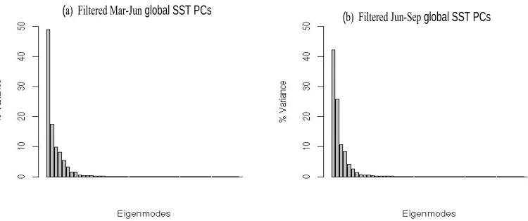
The percent variances explained by the PCs of the MAMJ and JJAS global SSTs are shown in Fig. 4. On the basis of North et al’s.(1982) delta-test, seven and four PCs for
MAMJ and JJAS, respectively, were statistically separate. These accounted for
(a) Unfiltered Mar-Junglobal SST PCs (b) Unfiltered Jun-Sep globalPCs
Table 2. As in Table 1, except for global SST PCs.
Seasons PC1 PC 2 PC 3 PC4 PC5 PC6 % Total
MAMJ 20.73 11.02 7.79 6.25 5.10 3.85 54.74
JJAS 17.08 10.85 7.33 4.42 - - 39.68
54.74% and 39.68%, respectively, of the unfiltered total variances. The contributions of the individual PCs are displayed in Table 2. To match the precipitation modes in order to facilitate comparison of the two seasons, the seven degenerate MAMJ global SST PCs were deliberately truncated to retain the first four, which explained 45.79% of the unfiltered total variance.
The eigenvectors (EOFs) and their time coefficients associated with the two seasons are presented in Figs. 5 and 6. The EOF 1 eigenvectors of MAMJ and JJAS, which explained 20.73% and 17.08% of their respective unfiltered total variances, are characterized by high positive weights over the global oceans, with the former season more pronounced than the latter (Figs. 5a and 6a). Their time coefficients, which show upward linear trends, are indicative of global warming signature (Ward, 1998; Folland et al., 1991). The eigenvectors
of MAMJ global SST EOF 2, which accounted for 11.02 % of the unfiltered total variance, depict the well-known ENSO mode (Fig. 5b,f) with its characteristic interannual oscillations (Folland et al., 1991; Ward, 1998). The global SST eigenvectors of JJAS EOF 2 explained
a. Unfiltered Mar-Jun globalSST EOF loadings 1 e. Unfiltered Mar-Jun global SST EOF 1 time series
b. Unfiltered Mar-Jun global SST EOF loadings 2
c. Unfiltered Mar-Jun global SST EOF loadings 3
f. Unfiltered Mar-Jun global SST EOF 2 time series
g. Unfiltered Mar-Jun global SST EOF 3 time series
d. Unfiltered Mar-Jun global SST EOF loadings 4 h. Unfiltered Mar-Jun global SST EOF 4 time series
a. Unfiltered Jun-Sep global SST EOF loadings 1
b. Unfiltered Jun-Sep global SST EOF loadings 2
c. Unfiltered Jun-Sep global SST EOF loadings 3
d. Unfiltered Jun-Sep global SST EOF loadings 4
e. Unfiltered Jun-Sep global SST EOF 1 time series
f. Unfiltered Jun-Sep global SST EOF 2 time series
g. Unfiltered Jun-Sep global SST EOF 3 time series
h. Unfiltered Jun-Sep global SST EOF 4 time series
The MAMJ and JJAS global SST EOF 3 eigenvectors (Figs. 5c and 6c) explained 7.79% and 7.33%, respectively, of their unfiltered total variances, and their time coefficients are dominated by interannual/decadal-like oscillations. In the case of global SST EOF 4, the unfiltered percent variances attributed to the eigenvectors of the MAMJ and JJAS seasons are 6.25% and 4.42%, respectively. The maximum centers of action of their anomaly patterns are depicted by high positive weights located over the tropical Atlantic and North Atlantic Oceans, eastern and western Pacific Oceans, which are in opposition to the negative weights over the south Pacific (Figs. 5d and 6d). Their time coefficients display decadal-like oscillations. Both the eigenvectors of these two modes of the two seasons show coherent patterns, which are reminiscent of the interhemispheric SST asymmetry found in previous studies (e.g., Lough, 1986; Folland et al., 1991; Ward, 1998).
3.1.3 MAMJ/JJAS West Africa rainfall and MAMJ/JJAS global SST relationships The associations between local/remote oceanic anomalies and tropical African rainfall variability on different time scales have been investigated by different authors (e.g., Lamb 1978a,b; Lough, 1986; Folland et al., 1986; Semazzi et al., 1996; Polo et al, 2008 ). Here, the
Table 3. Correlation between unfiltered West African MAMJ precipitation total time coefficients and climate indices. Bold-faced figures indicate statistical significance at 95 % confidence level. Numbers in parenthesis are correlations with detrended SST EOF 1 time coefficients.
Indices Precip. EOF 1 Precip. EOF 2 Precip. EOF 3 Precip. EOF 4
Nino 4 0.20 -0.18 -0.02 -0.25
Nino 3.4 0.09 -0.17 -0.04 -0.13
Nino 3 -0.08 -0.24 -0.07 -0.03
Nino 1+2 -0.12 -0.26 -0.04 0.02
ONI 0.16 -0.28 -0.10 -0.16
MEI 0.03 -0.28 -0.05 -0.13
BEST 0.14 -0.24 -0.14 -0.06
TNA 0.18 0.00 0.19 -0.09
TSA -0.24 -0.33 0.11 -0.20
TADM 0.31 0.23 0.07 0.07
AMO 0.22 -0.07 0.15 0.06
SOI -0.10 0.26 0.12 0.04
AT SST EOF 1 0.27 -0.08 0.25 0.08
AMM 0.28 0.17 0.14 0.02
IOSSDMAMJ -0.13 -0.51 0.05 -0.20
Global SST EOF 1 -0.19 (-0.10) -0.55 (0.16) 0.13 (-0.08) -0.15 (0.10)
Global SST EOF 2 0.10 0.03 -0.28 -0.08
Global SST EOF 3 -0.33 -0.12 -0.18 0.03
Global SST EOF 4 0.25 -0.02 0.04 0.14
Table 4. As in Table 3, except for JJAS. Indices Precip.
EOF 1 Precip. EOF 2 Precip. EOF 3 Precip. EOF 4
Nino 4 -0.31 -0.32 0.10 -0.04
Nino 3.4 -0.31 -0.25 0.02 -0.07
Nino 3 -0.34 -0.24 0.02 -0.09
Nino 1+2 -0.27 -0.21 -0.05 0.05
ONI -0.37 -0.09 0.08 -0.27
MEI -0.47 -0.33 0.16 -0.01
BEST -0.38 -0.20 0.09 -0.08
TNA 0.11 -0.18 0.13 -0.02
TSA -0.27 0.33 0.45 -0.08
TADM 0.28 -0.37 -0.26 0.05
AMO 0.35 -0.02 0.23 -0.14
SOI 0.28 0.21 0.15 0.17
AT SST EOF 1 0.26 -0.13 0.23 -0.12
AMM 0.34 -0.11 -0.12 0.03
IOSSDJJAS -0.46 -0.32 0.34 0.03
Global SST EOF 1 -0.35 (0.15) -0.33 (-0.03) 0.49 ( 0.22) -0.17(-0.21)
Global SST EOF 2 0.38 0.26 0.02 -0.22
Global SST EOF 3 -0.44 -0.07 0.05 0.33
Global SST EOF 4 0.12 0.09 0.00 -0.03
Atlantic Oceans, in modulating West African precipitation has been documented (Lamb, 1978; Folland et al., 1986; Xie et al., 2005). The positive (negative) events of the TADM
are usually accompanied by precipitation enhancement (suppression) over West Africa (Lamb, 1978; Folland et al., 1986). The warm phase of the TADM is inversely related to
total precipitation time coefficients (Fig. 7a) shows that the precipitation mode 1 is
associated to a large extent with cold (warm) SSTAs of the Equatorial mode (EM)/ Atlantic Nino and southwestern Atlantic mode, and warm (cold) SSTAs of the North Atlantic Ocean. The primary and secondary candidates connected to the MAMJ precipitation EOF 2 mode are the global SST EOF 1 index (r=-0.51) and IOSSD (r= -0.55)(Table 3), respectively, which suggest that their cooling (warming) events coincide with above (below) average precipitation over West Africa. The grid point correlation (Fig. 7b) captures the basin-wide SSTA patterns in this regard. In the case of MAMJ precipitation EOF 3, it seen from Table 3 to be connected to global SST EOF 2 (r= -0.28), which reflects an ENSO mode (Fig. 5b). The cooling (warming) ENSO events, which are closely related to reduced (increased)
vertical wind shear, coincide with precipitation surplus (deficit) over the region. On the other hand, the grid point correlation links the precipitation mode to the warming (cooling) events of TNA mode (Fig. 7c). Even though the MAMJ precipitation EOF 4 time coefficients do not appear to be connected to any of the indices (Table 3), the grid point correlation captures the EM/southeastern Atlantic and northwestern Pacific modes, where cooling (warming) events lead to above (below) normal precipitation. As a whole, the detrended global SST EOF 1 time coefficients exhibited poor association with MAMJ West African precipitation EOF modes (Table 3).
a. Correlation between unfiltered WA Mar-Jun precip. EOF 1 time series and unfiltered Mar-Jun global SST anomalies
b. Correlation between unfiltered WA Mar-Jun precip. EOF 2 time series and unfiltered Mar-Jun global SST anomalies
d. Correlation between unfiltered WA Mar-Jun precip. EOF 4 time series and unfiltered Mar-Jun global SST anomalies
c. Correlation between unfiltered WA Mar-Jun precip. EOF 3 time series and unfiltered Mar-Jun global SST anomalies
a. Correlation between unfiltered WA Jun-Sep precip. EOF 1 time series and unfiltered Jun-Sep global SST anomalies
b. Correlation between unfiltered WA Jun-Sep precip. EOF 2 time series and unfiltered Jun-Sep global SST anomalies
c. Correlation between unfiltered WA Jun-Sep precip. EOF 3 time series and unfiltered Jun-Sep global SST anomalies
d. Correlation between unfiltered WA Jun-Sep precip. EOF 4 time series and global SST anomalies
SST EOF 3 index, which are associated with the SM/CM. These three climatic indices,
well represented in the grid point correlation (Fig. 8a), suggest that cooling (warming)
of the tropical western Pacific, tropical Atlantic (eastern, southwestern and southeastern), and Indian Ocean leads to above (below) normal precipitation over the Sahel (Ward, 1998; Semazzi et al. 1988;Giannini et al, 2005; Polo et al., 2008, García-Serrano et al., 2008). On
the contrary, as seen in Fig. 8a, warming (cooling) of the Mediterranean Sea enhances (suppresses) precipitation over Sahel, which corroborates the findings of previous studies (Folland et al., 1996;Ward, 1998; Polo et al., 2008, García-Serrano et al., 2008). These
authors pinpoint the role of moisture advection from the warm Mediterranean Sea SSTAs into the Sahelian zone in enhancing pluviogenesis. The JJAS precipitation spatial mode 2 (GOGCM), which is reminiscent of the JAS GOGCM of Ward (1998) and Giannini et al.(2005), anticorrelated with TADM (r= -0.37 ) (Table 4). This negative correlation
coefficient signifies the importance and presence of the equatorial cold tongue complex (CTC) during JJAS Sahelian rainy season that is associated with precipitation minimum over the humid GOGC (Vizy and Cook, 2001, Gu and Alder, 2004; Giannini et al.,2005). This
the region, which is reflected in the grid point correlation (Fig. 8c). Finally, the JJAS precipitation EOF 4 is seen to be connected to global SST EOF 3 index (r =0.33), whose spatial structure is characterized by interhemispheric asymmetry in SST pattern of opposite signs, which is well represented in Fig. 8d. Here, positive (negative) phase is associated with enhanced (suppressed) precipitation over the eastern part of West Africa and the opposite effect over Western Sahel (Fig. 3d). As in the case of the MAMJ season, weak correlations were observed between the detrended global SST time coefficients and the precipitation modes (Table 4).
3.2 Boreal Spring-Summer Tropospheric Circulation over West Africa
This section focuses on the generalized (unfiltered) 3-D anomalous circulation patterns associated with the monsoon and middle layers during boreal spring-summer WAM represented by three isobaric surfaces, namely, the surface (1000 hPa), 850 hPa, and 500 hPa, where atmospheric moisture is relatively abundant as compared with other higher levels. In order to understand the physical relationships between WAM and SSTA patterns, composite analysis was applied to provide an insight for a description of the circulation regimes on the basis of the positive (negative) events associated with the precipitation modes. The description of the tropospheric circulation will be confined to the domain circumscribed by 50oW-90oE (lon), 40oS-40oN (lat), which captures the whole of African continent, the Indian Ocean and most parts of the tropical Atlantic.
3.2.1 Unfiltered surface circulation mechanism
The climate anomaly patterns of the two seasons computed are presented in Figs. 9 and 10. For the sake of convenience, all the positive (negative) events associated with the WAM circulation of the MAMJ and JJAS seasons, will hereafter be donated by the suffices pos# and neg#, where “#” denotes the precipitation time coefficients e.g.,1, 2, 3, etc.
The key anomalous circulation features associated with MAMJ pos1 (Fig.9a) may be described as the involvement of moisture supply created by contrasting SSTA patterns in the tropical Atlantic Ocean and the Mediterranean Sea, large-scale low-level cross-equatorial moisture flux convergence, and low-level cyclonic flows. Specifically, the mechanism leading to the ubiquitous positive rainfall anomalies over West Africa entails the interactions between anomalously strong surface winds driven by southwesterly basic-state flows, TNA meridional SST gradient, TADM, moderately warm Mediterranean Sea SSTAs, a moderately developed CTC in the tropical eastern Atlantic, whose evolution (formation, development and damping) is ascribed to the Angola/Benguela upwelling region located in the southeastern Atlantic Ocean (Folland et al., 1996;Ward, 1998; Polo et al. 2008) and
low-level cyclonic flow over West Africa, generated by diabatic heating, culminating in enhanced convection over West African region ( Vizy and Cook, 2001; Gu and Alder, 2004; Xie et al.,
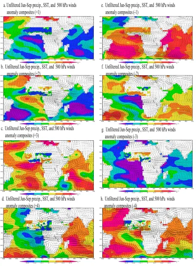
2005; Polo et al., 2008). The key circulation features of the JJAS pos1 events (Fig. 10a) are
moisture advection from warmer Mediterranean SSTAs, a weakening of the meridional tropical North Atlantic (TNA) SST gradient, and more intense surface winds, which consist of southerwesterlies and westerlies, depriving the humid GOGC of substantial precipitation (Giannini et al.,2005). The wetness of the Sahel during the JJAS season is also found to
coincide with colder Indian Ocean SSTAs, which corroborates the grid point correlation analysis (Fig. 8a), and previous studies ((Folland et al., 1996; Semazzi and Sud, 1996; Ward,
1998; Polo et al. 2008). The MAMJ neg1 and JJAS neg1 (Figs. 9e and 10e) events are the
antitheses of their respective positive events. The precipitation deficits in both cases are characterized by obliteration of the CTC, negative moisture advection and momentum transport from land into the Atlantic Ocean, warmer Indian Ocean SSTAs, reversal of surface winds and anticyclonic flows.
The salient anomalous circulation features of the MAMJ pos2 events (Fig. 9b) are depicted by an absence or a weak form of CTC in the Gulf of Guinea (GOG) accompanied by high evaporation, and strong low-level southwesterlies from the Atlantic accompanied by horizontal moisture advection over the GOGC, culminating in its anomalous wetness.
The above-normal GOGC precipitation is also found to have coincided with low-level cyclonic perturbations generated from anomalous West African heat lows, a well-developed CTC in the southern Atlantic and Indian Oceans. On the other hand, the JJAS pos2 events, which are typically the GOGM during the Sahelian rainy season (Giannini et al., 2005), is
a. Unfiltered Mar-Jun precip., SST, and sfc winds anomaly composites (+1)
b. Unfiltered Mar-Jun precip., SST, and sfc winds anomaly composites (+2)
c. Unfiltered Mar-Jun precip., SST, and sfc winds anomaly composites (+3)
anomaly composites (-1)
e. Unfiltered Mar-Jun precip., SST, and sfc winds
f. Unfiltered Mar-Jun precip., SST, and sfc winds anomaly composites (-2)
g. Unfiltered Mar-Jun precip., SST, and sfc winds anomaly composites (-3)
d. Unfiltered Mar_Jun precip., SST, and sfc winds anomaly composites (+4)
h. Unfiltered Mar_Jun precip., SST, and sfc winds anomaly composites (-4)
a. Unfiltered Jun-Sep precip., SST, and sfc winds anomaly composites (+1)
e. Unfiltered Jun-Sep precip., SST, and sfc winds anomaly composites (-1)
b. Unfiltered Jun-Sep precip., SST, and sfc winds anomaly composites (+2)
f. Unfiltered Jun-Sep precip., SST, and sfc winds anomaly composites (-2)
c. Unfiltered Jun-Sep precip., SST, and sfc winds
anomaly composites (+3) g. Unfiltered Jun_Sep precip., SST, and sfc windsanomaly composites (-3)
d. Unfiltered Jun-Sep precip., SST, and sfc winds anomaly composites (+4)
h. Unfiltered Jun-Sep precip., SST, and sfc winds anomaly composites (-4)
a. Unfiltered Jun-Sep precip., SST, and sfc winds anomaly composites (+1)
e. Unfiltered Jun-Sep precip., SST, and sfc winds anomaly composites (-1)
b. Unfiltered Jun-Sep precip., SST, and sfc winds f. Unfiltered Jun-Sep precip., SST, and sfc winds anomaly composites (+2) anomaly composites (-2)
c. Unfiltered Jun-Sep precip., SST, and sfc winds
anomaly composites (+3) g. Unfiltered Jun_Sep precip., SST, and sfc windsanomaly composites (-3)
d. Unfiltered Jun-Sep precip., SST, and sfc winds anomaly composites (+4)
h. Unfiltered Jun-Sep precip., SST, and sfc winds anomaly composites (-4)