THE RATE OF DECREASE OF HETEROZYGOSITY IN A POPULATION OCCUPYING A CIRCULAR OR A LINEAR HABITAT

(1)

THE RATE O F DECREASE OF HETEROZYGOSITY IN A

POPULATION OCCUPYING A CIRCULAR OR A LINEAR HABITAT*

TAKE0 MARUYAMA

National Institute of Genetics, Mishima, Japan Received July IO, 1970

rate at which a finite population approaches homozygosity is an impor- 'Eft subject in population genetics. This problem was first investigated by

FISHER (1922, 1930) and by WRIGHT (1931).

WRIGHT

found the general result that the rate in a randomly mating population of N diploid individuals is equal to 1/(2N). Thus asymptotically the probability of a population being monomorphic is proportional to (1 -1/2N) t . This information plays a very important

role in the evolutionary theories advanced by

WRIGHT

(1931 and later) and by KIMURA (1968, 1969). ROBERTSON (1964) clarified the effect of nonrandom mating on this rate. Letting c and c* be, respectively, the probabilities that two homologous genes taken at random in a population are identical by descent, and, that two homologous genes taken one from each of the two individuals actually mated together are identical by descent, he showed

1 - C*&1 4N(1 - c t )

A = - -

where -A is the rate at which heterozygosity declines from generations t-1 to generation t. WRIGHT (1965) also considered a similar problem using his F

statistics and showed that in a circular mating system, the strong local differenti- ation interferes with the progress of fixation in the whole population.

I n this paper, we consider populations occupying a circular habitat or a linear habitat of finite length. Although a habitat need not be actually circular or linear, it is one-dimensional and of finite length. Assuming that mutation or migration is zero or negligibly small, and considering one locus, the rate a t which the whole population approaches homozygosity (becomes monomorphic) will be investigated. For both circular and linear habitats, we denote the length of a habitat by L and the population density by p. We assume that the organism under consideration is monoecious and diploid, and furthermore that individuals are distributed uniformly in the habitat. Therefore there are altogether pL diploid individuals in the whole population.

2. ANALYSIS FOR CIRCULAR HABITATS

Consider a circular habitat of length L. Let f ( t , x ) be the probability that two * Contribution No. 770 from the National Institute of Genetics, Mishima, Shizuoka-ken, Japan. Aided in part by a Grant-in-Aid from the Ministry of Education, Japan.

(2)

438 T. MARUYAMA

homologous genes which are a distance z apart at time t are identical by descent. Throughout this paper we assume that generation time is continuous, but the measure of the time is so adjusted that unit time corresponds to one generation. Now extend the probability function f ( t , x ) onto the whole interval (-m,m)

as a periodic function of period L, i.e., f ( t , z ) = f ( t , y ) if y = k L

+

x

for

k

= 0, AI, ‘2,

.

. . .

Let m ( ~ t , x ) be the probability density that a gene moves distance

z in time interval At. Positive z means going one direction, say to the right, and negative x means the opposite direction, in this case to the left. Throughout this paper, we assume (i) that migration function m(At,z) is continuous in z for all At, (ii) that it is symmetric for all At, i.e., m(At,s) = m(At,-x), and (iii) the variance of m ( ~ t , z ) for unit time is finite and we denote it by U . These assumptions are not strict for most biological situations. Now let

r(At,z> =

JYm

m(At,x--z)m(At,z)d-z. (2-1) r ( A t , x ) is the convolution of m(At,z) with itself, and in a circular habitat this function is the probability density that the distance between two genes changes by z in the time interval At. The movement is assumed to be stochastic.

By the assumption of no mutation nor migration from outside the population,

f ( t , z ) approaches unity as time increases. If we define h (t,z) = 1

-

f (t,z)

,

then h(t,z) converges to zero asymptotically. We are interested in the rate at which h(t,z) decreases with time, i.e., ah(t,z)/at for large t . Concerning h(t,z) we have the following equation:

AtS

(z-Z)

h ( t + ~ t , z ) = r at,^) [ h (t,x--z) - h ( t , ~ - ~ ) ] d ~

+

o ( A t ) (2-2)

2P

where 6 (.) is Dirac’s delta function. This equation is analogous to equation (2-9) in

MALBCOT

(1967). From (2-2), we have a partial differential equation

(For a derivation of (2-3) from (2-2), see APPENDIX.)

Now our interest is to determine the dominant eigenvalue and its associated eigenfunction of the right side of (2-3). For a fixed value of density p, if we let

L be large, h(t,O) = h(t,L) 0 asymptotically, because homozygosity proceeds locally much faster than that in the whole habitat when L is large and/or U is small. In such a circumstance we have on the right side of (2-3), the operator,

a 2

ax2 U-

to which we seek the eigenvalue, and the boundary condition to be imposed is

4

(0) =

4

( L ) = 0. Therefore the dominant eigenvalue is U T 2

L2

’

A = - - _(2-4)

(3)

MIGRATION A N D GENETIC VARIANCE 439

(see TITCHMARSH 1962, Ch. I ) .

This means that for a large value of L, or equivalently for a small value of U , the asymptotic form of h ( t , x ) is proportional to +(x) of ( 2 - 5 ) and it decreases at the rate ur2/L2. In other words, if the habitat is large, or the migration distance is small, asymptotically h ( t , x ) cc e-(o+/L2)t sin

-

.

It

is important that this rate is independent of the total number of individuals in the population but proportional to the variance of migration distance divided by the square of the length of habitat. I t is also worthwhile to note that, as long as the assumptions

(i) - (iii) hold, the decreasing rate and the form of h ( t , x ) are independent of the pattern of the migration.

From the foregoing analysis it follows that the effective size of a population can become arbitrarily large without the population actually having a large number of individuals and such a population may maintain a larger amount of genetic variation than a panmictic population of the same actual size (for the effective size of a population see KIMURA and CROW 1963). It is also important to note that such a population has a slower rate of random drift in gene fre- quencies, and therefore the time required for gene substitutions may be much longer than in a panmictic population (see KIMURA and OHTA 1969).

On the other hand, for fixed L, if we assume p = 00, we have a situation where

the whole population is of infinite size and the rate of decrease in genetic variability is zero. Now consider a real situation with a finite value of p as a perturbation of the above hypothetical case with p = w . Then we can apply pertur-

bation theory to estimate the eigenvalues of the right side of ( 2 - 3 ) . The first- order perturbation to the dominant eigenvalue of ( 2 - 3 ) is given by

T X

L

1

A ” - - -

2LP

.

(For a derivation and for a higher-order approximation see APPENDIX.) Notice that for the first-order approximation, the dominant eigenvalue is equal to that of the panmictic population of size Lp. The second- o r higher-order terms in ( 2 - 6 ) are more difficult to compute. But biologically, it is more important to know the range of p for which the approximation formula ( 2 - 6 ) is valid because it tells us whether a particular population can be considered as a panmictic population or not. According to the perturbation theory, approximation (2-6) is valid, if 1/2Lp is less than ar2/L2. Therefore if 1/2Lp

<

uT2/L2, the situation can be considered approximately as a panmictic population of size Lp. For such cases, we can also determine the eigenfunction by the perturbation method. If

(4)

440 T . M A R U Y A M A

a constant function. (For a higher-order approximation see APPENDIX.) It will be shown in section 4 that when 1/2Lp

>

urr2/L2, the dominant eigenvalue is

approximated by u2/L2.

3. ANALYSIS FOR L I N E A R HABITATS

Let us now consider a one-dimensional habitat with two end points. W e assume the length of the habitat is finite and denote it by L. Unlike the situations treated in the previous section, the space is not homogeneous, so the probability of being identical by descent cannot be specified as a function of distance between genes alone; we need to specify the location of each of two genes. Therefore let f ( t , x , y ) be the probability that two homologous genes, one at location x and the other at location y at time t, are identical by descent, where 0 5 x,

y

i

L. Although the actual habitat consists of line segment [O,L] and although the probability function f ( t , x , y ) with respect to x and y is defined on the rectangle [O,L]X[O,L], we can extend f ( t , x , y ) onto the whole plane. First we extend f(t,z,y) onto the rectangle [-L,L]X [-L,L] by f ( t , - x , y ) f ( t , x , y ) , f(t,x,-y) =f(t,z,y), and f ( t , - x , - y ) = f ( t , x , y ) for 0 5 x, y 5 L. Then we extend this f ( t , x , y ) defined on -L

i

x, y 5 L, onto the whole plane as a doubly periodic function of period 2L, where the fundamental period-parallelogram is x =

*

L and y = *L.

Let m(At,z) be the migration function defined in section 2. With this setup, we have

h (t+at,x,y) =

JIm

m(at,z) m (at,w) h (t,x--z,y-w) dzdw

And analogous to (2-3),

Our interest is to determine the dominant eigenvalue and its associated eigenfunction for the right side of (3-2). For a fixed value of p, if we let L get indefi- nitely large, h(t,x,x) N 0 for the same reason as in the previous section. Thus when L is large and/or U is small, the boundary condition to be imposed on the eigenfunction is

( 3 - 3 )

With this boundary condition the second term on the right side of (3-2) vanishes, and the operator for which we want to determine eigenvalues becomes

+(x,y)

= 0 for y = + x

*

k L ,

k =

0 , 1, 2,

. . .

.

(3-4)

with the boundary condition ( 3 - 3 ) .

x and y into new variables z and w as follows:

(5)

MIGRATION A N D GENETIC VARIANCE 4 4 1

Then (3-4) is changed to

(3-5)

and the boundary condition is changed to

(3-6)

This is a well-known equation (see

TITCHMARSH

1958, Ch.

XI).

With this boundary condition, the dominant eigenvalue which we seek is

+(w,z)

= O

for z,w=O, ‘1, ‘ 2 ,

. . . .

(3-7)

(3-8)

Therefore when the habitat is large or the migration distance is small, the genetic variation in a population decreases asymptotically at the rate u 2/2L2 ,

which is half of the rate for the case where the habitat is circular.

Let us next consider the other extreme situation, namely p = W . As in the previous section, applying the perturbation method for a finite value of p , we have the first-order approximation

which is valid if 1/2Lp

<

,r2/2L2. Similary the first-order perturbation of the associated eigenfunction is

(3-10)

a constant function. (For higher-order approximations see APPENDIX.) There- fore, we have arrived at a conclusion similar to that of the previous section. Thus when 1/2Lp

<

,2/2L2, the population can be considered as a panmictic population of size pL, as far as the decrease in the genetic variability or approach to homozygosity is concerned. On the other hand, when the inequality is reversed, the rate is approximately equal to ur2/2L2.

4. TRANSITION F R O M H I G H DENSITY TO LOW DENSITY

In sections 2 and 3 it was shown that for a large habitat or small V, the asymp-

(6)

442 T. MARUYAMA

density the rate for either habitat is approximately 1/2Lp, which is the rate in a panmictic population of size Lp. It is important to note that the approximations series (2-6) and (3-9) are valid in the range 1/2Lp

<

ur2/L2 (circular habitat) and 1/2Lp

<

m2/2LZ (linear habitat). Thus it is reasonable to conjecture that the values of the parameters for which

U 2

- - -

1 - (circular habitat)

2Lp L2

m 2

1 - (linear habitat)

2Lp 2L2

are turning points at which one approximation formula breaks down and the other formula becomes valid. Namely, the rate is most closely approximated by

m2/L2 (circular) and ur2/2L2 (linear) if the value on the left side of (4-1) is smaller than that on the right side, and it is most closely approximated by 1/2Lp

if the inequality is reversed. This conjecture is supported by numerical evidences given in the next section.

5. SOME NUMERICAL CALCULATIONS

In order to check the validity of the preceding analyses,

I

have performed some numerical calculation based on the following scheme derived from (2-2) and

(3-1). Letting At = 1,

ht(x)

= h ( t , x ) ,

ht(x,y)

= h(t,x,y), (2-2) and (3-1) are changed to

and

respectively, where m (2) = m ( A t , x ) and

m

Since L and U are relative, in this section we fix L = 1 without loss of generality.

It is easy to carry out these iterations numerically for a given migration function m ( x ) . The functions used as a migration function are normal,

exponential,

(7)

MIGRATION AND GENETIC VARIANCE

and uniform distribution

443

(5-5)

For given values of the parameters and migration function, the iteration is started with the initial functions

h o ( z )

= 1 for (5-1) and h,(x,y) = 1 for (5-2).

After each iteration the functions are normalized according to the norm m ( s ) = 0 otherwise.

or

depending on the number of variables. Iteration is continued until the ratios of the norms of functions in consecutive iterations become constant, i.e.,

Of course this equality cannot be attained unless we start the iteration with an eigenfunction. The iteration is therefore stopped when

When this inequality is attained, the ratio

11

ht+l

11 /

11

ht

11

is the dominant eigenvalue of the transformations

(5-1)

or

(5-2).

Therefore this ratio minus unity is the corresponding value to that given in (2-4), (2-6), (3-7), or (3-9).

There is good agreement between the values obtained by the theoretical formulas and those obtained by the numerical iteration. A few examples of the comparisons are presented in Tables 1 and 2. There is also good agreement between the associated eigenfunctions determined theoretically by (2-5), (2-7)

,

(3-8), or (3-IO), and those obtained numerically by the iterations. Some comparisons are presented in Tables 3-6.

Transitional behavior of the dominant eigenvalues from ax2/L2 (circular) or

ur2/2L2 (linear) to 1/2Lp is shown in Figures 14. In all the figures the vertical axis stands for the dominant eigenvalue. Since there are two parameters, p and

U, we fix the value for one parameter and let the other vary. First we consider

examples where we fix p and let U vary from to IC1. In these cases the values

from the approximation formula 1/2Lp remain constant, since it is independent of U; whereas the values from the approximation formulas ur2/L2 and m2/2L2

change as U varies. In Figures 1 and 2 the horizontal axis stands for U, the

(8)

444 T. MARUYAMA

al

c -4 b

m

>

E -

O m

l c i l

- 4 m

c - 3

.-

C - 0 1 a m X ' w 4 - a m E l M m 0 - z X - O r - M I a m a- 4

E-

O m W I

4 VI

(9)

MIGRATION A N D GENETIC VARIANCE

E -

OU, W I

--I Kl c -

3

c -

O *

a1

X K l w -

rl

& I 1 O W z -

g;

x

0 - u m a l a m A - E &I-

O U , W I

.-I U,

c - 3

c -

O *

a l

X U , w - d - m m E l &!U, 0- z X - o w

(10)

446

T. MARUYAMA

TABLE 3

Comparison of the eigenjunction giuen by ( 2 - 5 ) with the eigenfunctions obtained by the numerical iteration (5-1)

The parameters are U = 0.001 and 2pL = 30.

Approx. Normal Expon. Uniform

( 2 - 5 ) ( 5 - 3 ) ( 5 - 4 ) ( 5 - 5 )

x \

0

0 . 0 4

0.08

0.12

0.16

0 . 2 4

0 . 3 2

0 . 4 0

0 . 4 8

0

0.0267

0 . 0 5 2 9

0 . 0 7 8 3

0 . 1 0 2 5

0 . 1 4 5 6

0 . 1 7 9 6

0 . 2 0 2 3

0 . 2 1 2 3

0 . 0 0 3 0

0 . 0 1 9 2

0 . 0 4 4 6

0 . 0 7 1 8

0 . 0 9 6 5

0 . 1 4 5 8

0 . 1 8 5 0

0 . 2 1 1 3

0 . 2 2 3 0

0 . 0 0 3 6

0 . 0 2 0 5

0.0465

0 . 0 7 5 3

0 . 0 9 9 2

0 . 1 4 5 8

0 . 1 8 2 6

0 . 2 0 7 3

0 . 2 1 8 2

0 . 0 0 3 4

0 . 0 1 8 7

0 . 0 4 4 6

0 . 0 7 1 5

0 . 0 9 6 3

0 . 1 4 5 8

0 . 1 8 5 1

0 . 2 1 1 4

0 . 2 2 3 1

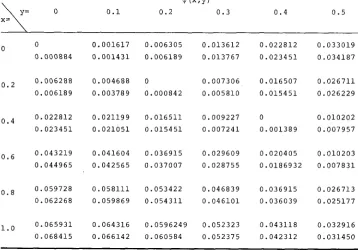
TABLE 4

Comparison of the eigenfunction giuen by (3-8), upper figure, with the eigenjunction obtained

by the iteration (5-2), lower figure, using uniform migration function (5-5) with U = 0.001 and 2pL = I O .

@ (XnY)

0 0 . 1 0 . 2 0 . 3 0.4 0 . 5

X= \=

0

0 . 0 0 0 8 8 4

0

o.2 0 . 0 0 6 2 8 8 0 . 0 0 6 1 8 9

0 . 0 2 2 8 1 2

0 . 0 2 3 4 5 1 0.4

o . 6 0 . 0 4 3 2 1 9 0 . 0 4 4 9 6 5

o.8 0 . 0 5 9 7 2 8 0 . 0 6 2 2 6 8

0 . 0 6 5 9 3 1

0 . 0 6 8 4 1 5

1.0

0 . 0 0 1 6 1 7 0 . 0 0 6 3 0 5 0 . 0 1 3 6 1 2

0 . 0 0 1 4 3 1 0 . 0 0 6 1 8 9 0 . 0 1 3 7 6 7

0 . 0 0 4 6 8 8 0 0 . 0 0 7 3 0 6

0 . 0 0 3 7 8 9 0 . 0 0 0 8 4 2 0 . 0 0 5 8 1 0

0 . 0 2 1 1 9 9 0 . 0 1 6 5 1 1 0 . 0 0 9 2 2 7

0 . 0 2 1 0 5 1 0 . 0 1 5 4 5 1 0 . 0 0 7 2 4 1

0 . 0 4 1 6 0 4 0 . 0 3 6 9 1 5 0 . 0 2 9 6 0 9

0 . 0 4 2 5 6 5 0 . 0 3 7 0 0 7 0 . 0 2 8 7 5 5

0 . 0 5 8 1 1 1 0 . 0 5 3 4 2 2 0 . 0 4 6 8 3 9

0 . 0 5 9 8 6 9 0 . 0 5 4 3 1 1 0 . 0 4 6 1 0 1

0 . 0 6 4 3 1 6 0 . 0 5 9 6 2 4 9 0 . 0 5 2 3 2 3

0 . 0 6 6 1 4 2 0 . 0 6 0 5 8 4 0 . 0 5 2 3 7 5

0 . 0 2 2 8 1 2 0 . 0 3 3 0 1 9

0 . 0 2 3 4 5 1 0 . 0 3 4 1 8 7

0 . 0 1 6 5 0 7 0 . 0 2 6 7 1 1

0 . 0 1 5 4 5 1 0 . 0 2 6 2 2 9

0 0 . 0 1 0 2 0 2

0 . 0 0 1 3 8 9 0 . 0 0 7 9 5 7

0 . 0 2 0 4 0 5 0 . 0 1 0 2 0 3

0 . 0 1 8 6 9 3 2 0 . 0 0 7 8 3 1

0 . 0 3 6 9 1 5 0 . 0 2 6 7 1 3

0 . 0 3 6 0 3 9 0 . 0 2 5 1 7 7

0 . 0 4 3 1 1 8 0 . 0 3 2 9 1 6

(11)

MIGRATION A N D GENETIC VARIANCE 4 4 7

TABLE 5

Comparison of the eigenfunction given b y (2-7) with the eigenfunctions obtained b y the numerical iteration (5-1).

The parameters are U = 0.1 and 2pL z 100.

Approx. Normal Expon

.

Uniform

(2-7) (5-3) (5-4) ( 5 - 5 )

0 0.04 0.08 0.12 0.16 0.24 0.32 0.40 0.48 0.1111 0.1111 0.1111 0.1111 0.1111 0.1111 0.1111 0.1111 0.1111 0.1052 0.1071 0.1075 0.1094 0.1107 0.1131 0.1148 0.1159 0.1163 0.0099 0.1050 0.1076 0.1101 0.1120

0 . U 4 4

0.1162 0.1174 0.11785 0.1057 0.1058 0.1074 0.1090 0.1106 0.1132 0.1151 0.1163 0.1169

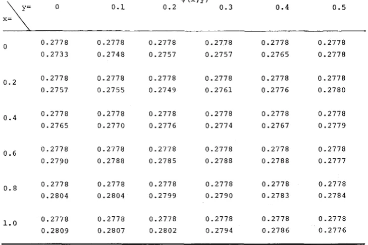
TABLE 6

Comparison of the eigenfunction given b y (3-IO), upper figure, with the eigenfunction obtained b y the iteration ( 5 - 2 ) , lower figure, using normal migration function (5-3)

with U = 0.1 and 2pL = 100.

0 k , Y )

0 0.1 0.2 0.3 0.4 0.5

0.2778

0.2733 0

o.2 0.2778

0.2757

o . 4 0.2778

0.2765

o.6 0.2778

0.2790

o.8 0.2778

0.2804 0.2778 0.2809 1.0 0.2778 0.2748 0.2778 0.2755 0.2778 0.2770 0.2778 0.2788 0.2778 0.2804 0.2778 0.2807 0.2778 0.2757 0.2778 0.2749 0.2778 0.2776 0.2778 0.2785 0.2778 0.2799 0.2778 0.2802

0. 27.7 8

(12)

448 T . MARUYAMA

small values of U ; and at the neighborhood of the point where the two lines

meet, they turn and follow the line given by 1/2p. In Figures 3 and

4,

we fix the values of U and let p vary from 10 to lo4. Thus in these figures, approximation

formulas ur2/L2 and ur2/2L2 assume constant values, but the value of formula 1/2p changes as p varies. From this numerical evidence, together with analysis developed in sections 2 and 3, we may conclude that approximation formulas (2-4) and (2-5) or (3-7) and (3-8) are valid f o r situations where ur2/L2

<

1/2Lp or ur2/2L2

<

1/2Lp holds; while approximation formulas (2-6) and (2-7) o r (3-9) and (3-10) are valid for situations where

m2/L2

>

1/2Lp or ur2/2L2

>

1/2Lp. A set of parameters for which ur2/L2 = 1/2Lp or ur2/2L2 = 1/2Lp holds

Linear Habitat

io4 I I I I

I 6' I 6' I IO2 16'

d

FIGURES 1 and 2.-The vertical axis stands for the largest eigenvalue (-A) of (2-2) or (3-1). The horizontal axis stands for the variance of migration distance (U). L is the length of the

(13)

MIGRATION AND GENETIC VARIANCE

lfj2

x

I

1 6 ~

I fj4

449

dlr2/L*

I

\

-

1 I I

3 t

lo4

x

I 0"

6-0.001

Linear Habltat

l o ' ,

3

10

Id

io3 I$

2 f L

FIGURES 3 and %--The same as Figures 1 and 2, except that the horizontal axes stand for the population size (2pL).

represents a turning point, in that the validity of one approximation formula breaks down at this point and the other formula becomes more valid from this point on. All the numerical examples seem to indicate that transition behavior

of the eigenvalues in the sense discussed above takes place rapidly, at least in the region of biological interest. This implies that the approximation formulas given in this report cover most of the biologically significant cases.

(14)

450 T. MARUYAMA

SUMMARY

The asymptotic rate a t which a population occupying a circular or linear habitat approaches homozygosity was investigated. If L is the length of the habitat, p the population density, and U the variance of the migration distance

in one generation, the rate is approximately equal to

when the inequality

(circular),

U T 2 1

L2 2Lp

-<-

(circular),

U T 2

2L2

- (linear)

f J - 2 1

2L2 2Lp

-<-

(linear)

holds. Thus for these cases the rate is proportional to the migration distance divided by the square of the length of the habitat, but it is independent of the population size (number of individuals in a population). When the inequality is reversed, the rate is approximately equal to 1/(2Lp).

Thus it is equal to the rate in a panmictic population of size Lp, which implies that the effect of geographical structure of the population disappears as far as the rate of decrease in the genetic variability in the whole population is concerned.-Approximation formulas for the eigenfunctions associated with the dominant eigenvalues were also obtained.-The validity of the analyses were checked by numerical calculations.

LITERATURE CITED

FISHER, R. A., 1922 On the dominance ratio. Proc. Roy. Soc. Edinburgh B: 42: 321-341. The distribution of gene ratio for rare mutations. Proc. Roy. S o c . Edinburgh B:

Diffusion Processes and their Sample Paths. Springer-

-,

50: 205-220.

Verlag, New York. 1930

ITO, K. and H. P. MCKEAN, JR., 1965

KATO, T., 1966 Perturbation Theory for Linear Operators. Springer-Verlag, New York.

KIMURA, M., 1968 Evolutionary rate at the molecular level. Nature 217: 624426. -, 1969 The rate of molecular evolution considered from the standpoint of population genetics.

Proc. Nad. Acad. Sci. U.S.63: 1181-1188.

KIMURA, M. and J. F. CROW, 1963 The measurement of effective population number. Evolution

KIMURA, M. and T. OHTA, 1969 The average number of generations until fixation of a mutant gene in a finite population. Genetics 61 : 763-771.

MAL~COT, G., 1967 Identical loci and relationship. Proc. 5th Berkeley Symp. Math. Statis. Prob. 4: 317-332.

ROBERTSON, A., 1964 The effect of nonrandom mating within inbred lines on the rate of inbreeding. Genet. Res. 5 : 164-167.

TITCHMARSH, E. C., Eigenfunction Expansions Associated with Second-Order Differential Equa- tions. Part one, second edition, 1962. Part two, 1958. Clarendon Press, Oxford.

WRIGHT, S., 1931 Evolution in Mendelian populations. Genetics 16: 97-159. ---, 1965 The interpretation of population structure by F-statistics with special regard to systems of mating. Evolution 19: 395-420.

(15)

45

1

Appendix

D e r i v a t i o n o f ( 2 - 3 ) f r o m ( 2 - 2 )

Assumption ( i ) o f s e c t i o n 2 i m p l i e s t h a t f o r any

g i v e n E > 0

see I t o a n d McKean ( 1 9 6 5 ) f o r a p r o o f . Then ( A . 1 ) and

a s s u m p t i o n (iii) i m p l y t h a t t h e f o l l o w i n g l i m i t i s

i n d e p e n d e n t o f E > 0 a n d

Expand h ( t , x - z ) of ( 2 - 2 ) i n t o T a y l o r s e r i e s

Then f o r any g i v e n E > 0 , l e t 6 b e s u c h t h a t

D i v i d e t h e i n t e g r a l on t h e r i g h t s i d e of ( 2 - 2 ) i n t o t w o

(16)

452 T. MARUYAMA

At, we have

1

L{

h(t+At,x)

-

At

-

1

r(At,z)h(t,x-z)dz

- -

a h

1

zr(At,z)dz r (At,z) h (t ,x)dz

1 2 1 < 6

IzI<6 ax at

1z1>6 At

+ - - - 1 a2h 1

2 ax2 At z 2 r(At,z)dz

+

- -

1

z2r(At,z)R(t,x,z)dz

I

z 1 < 6

2 At 1z1<6

Since r(At,z) + 6(x) Dirac's delta function, as At + 0,

the left side of (A.4) converges to

at

ah and I -1

5 to -6 2P (x)h(t,x), as At + 0. By (A.1) and boundedness of h(t,x) I + 0,

1

by assumption (ii) of section 2 I = 0, by (A.2) 2

a

Lh

2

+ U

-

,

and by (A.2) and ( A . 3 ) [ I 4 [ < €0 in which

ax

E can be made arbitrary small. Therefore we obtain ( 2 - 3 )

from (2-2). Similary we can also derive (3-2) from ( 3 - 1 ) .

Approximation by perturbation method

(17)

becomes

453 a'

u - ₂

ax

(2-3) w i t h a f i n i t e v a l u e o f p c a n b e t h e n c o n s i d e r e d a s

a p e r t u r b e d form o f ( A . 5 ) . I t i s e a s y t o o b t a i n t h e c o m p l e t e

s p e c t r a l a n a l y s i s f o r ( A . 5 ) . They a r e

1

Q ( x ) =

-

J L

0

2vnx

On(x) =

E

c o s

-

L n = 1, 2 , 3 , a - .

and t h e a s s o c i a t e d e i g e n v a l u e s a r e

A p p l y i n g t h e p e r t u r b a t i o n t h e o r y , t h e dominant e i g e n v a l u e

(18)

454

T . MARUYAMA

and t h e a s s o c i a t e d e i g e n f u n c t i o n

@ ( X I

c a n b e a l s o expanded a s

The p e r t u r b a t i o n s e r i e s ( A . 6 ) and (A.7) a r e c o n v e r g e n t 2

'

2"

.

The s e r i e s e x p a n s i o n of t h e d o m i n a n t

1

i f - < - 2PL L

e i g e n v a l u e € o r t h e case of a l i n e a r h a b i t a t i s

2

I T 0

.

See Kat0 (1966) f o r which i s c o n v e r g e n t i f

-

1 <

-

2 p L 2L