ABSTRACT
MOORE, CHRISTOPHER CLAYTON. Using Empirical Benefit Estimates in a Bioeconomic Model of Invasive Species Control. (Under the Direction of Daniel J. Phaneuf and Walter N. Thurman.)
The hemlock woolly adelgid (HWA) is a destructive invasive insect that is threatening hemlock forests in the eastern United States. This research combines results from a US Forest Service effort to value hemlock decline in the southern Appalachian Mountains with a dynamic model of ecosystem services to evaluate a mitigation strategy that has been proposed for three federal lands in western North Carolina. Resource managers plan to use chemical insecticide and introduce nonnative predators of HWA to a network of treatment sites in Great Smoky Mountain National Park, Pisgah National Forest, and Nantahala National Forest. The bioeconomic model developed here estimates a net present value for the proposed strategy and suggests a more efficient allocation of limited conservation resources.
Using Empirical Benefit Estimates in a Bioeconomic Model of Invasive Species Control
by
Christopher C. Moore
A dissertation submitted to the Graduate Faculty of North Carolina State University
in partial fulfillment of the requirements for the Degree of
Doctor of Philosophy
Economics
Raleigh, North Carolina 2008
APPROVED BY:
__________________________ __________________________
Daniel J. Phaneuf Walter N. Thurman
(Co-Chair of Advisory Committee) (Co-Chair of Advisory Committee)
__________________________ __________________________
Martin D. Smith Thomas P. Holmes
DEDICATION
To my wife Stephanie for her endless support and patience
BIOGRAPHY
Christopher Clayton Moore spent his childhood in Princeton, New Jersey with parents Richard and Linda and sister Michele. After earning a Bachelor’s degree from Elon University in North Carolina he began his career in environmental economics, joining Triangle Economic Research as an Associate Economist. After two years with the environmental economics consulting firm and a brief stint as a bar tender, Christopher accepted a National Needs Research Fellowship to pursue a doctorate in economics at North Carolina State University.
Christopher continues his research at the Environmental Protection Agency’s National Center for Environmental Economics. He now resides in the
ACKOWLEDGEMENTS
I would like to acknowledge the gentlemen of my dissertation committee for their guidance and support. In particular, Dan Phanaeuf served as my co-chair and a shining example of a family man and economist. Wally Thurman is a tremendous resource, no matter the subject. Marty Smith deserves my thanks for introducing me to the fascinating area of bioeconomics and, as a pillar of the field, was an invaluable member of my committee. Tom Holmes brought me onto the
Hemlock Project and took me seriously when he had no reason to. Ray Palmquist was my first graduate school professor and the first person to shake my hand after my defense, thank you.
It has been a pleasure working with Kathleen Bell on the Hemlock Project and I look forward to continuing our collaboration. During my brief visit to UNR Klaus Moeltner shared Bayesian insight and valuable lines of code, both of which shaped this analysis. Jake Brimlow and Alex Marten, two of my colleagues at NC State, have been generous with feedback, advice, and Matlab code.
I thank my parents, Richard and Linda, for their constant encouragement. Not just in this, my latest endeavor, but in all my efforts that have contributed to my character.
TABLE OF CONTENTS Page List of Tables……….………...
List of Figures……….………..
1. Introduction………..………..
2. Hemlock Woolly Adelgid ……….……….
I. Infestation History……….
II. Biology………...
III. Hemlock Resources………...…………
IV. Control Options……….…………
V. Study Area………...
3. Survey Design and Administration……… I. Valuing Hemlock Decline..……….………..
II. The Valuation Question……….…………
(A) The Good Being Valued……….……..
(B) Valuation Approach……….
(C) Response Format………..……
(D) Multiple Valuation Questions on a Single Survey………
(E) Information Section………..
(F) Follow-Up Questions………
III. Survey Administration………..
4. Benefits Estimation……….
I. Estimation Approach……….………
II. Modeling Assumptions………..………
(A) The Data Generating Process……… (B) The Likelihood Function………..……… (C) Form of the Willingness-to-Pay Function………
III. Single-Equation Models………
(A) Ordinary Least Squares Estimation of Interval Response Data…… (B) Maximum Likelihood Estimation of Interval Response Data…..… IV. Bayesian Estimation of the Multiple-Equation Model…………..……… (A) Derivation of the Joint Posterior………..………… (B) Drawing from the Full Conditional Distributions………
(C) Gibbs Sampler Results……….……
(D) Specification Analysis………..……… V. Allocating Mitigation Resources………...
VI. Discussion………....………...
5. The Bioeconomic Model………
I. Dynamic Policy Analysis………..………
II. The Dynamic Population Model……… (A) Defining the State and Control Variables……….……… (B) Specifying a Dynamic Population Model………….……… (C) Parameterizing the Dynamic Model……….………
(i) Hemlock Carrying Capacity and Sustenance Parameters… (ii) One-Species Simulations: Intrinsic Growth Parameters..… (iii) Two-Species Simulations: Predation Parameters…….…… (iv) Chemical Insecticide Decay Parameter……… III. Specifying the Instantaneous Net Benefit Function…………..………… IV. Policy Simulation and Evaluation……….……… (A) Defining Policy Parameters for Simulation……….………… (B) Computer Simulation of Proposed Policy……….………...
V. Bayesian Policy Analysis………...………
VI. Discussion ……….………..…..
6. Key Findings and Research Extensions……….……… I. Contributions to Several Areas of Scholarship………. II. Nonmarket Valuation Survey Design and Administration………
III. Applied Econometrics………
IV. Bioeconomic Model………..
References………..………..
Appendix: Southern Appalachian Forest Management Survey……… 108 110
112 113 113 115 117
119
LIST OF TABLES
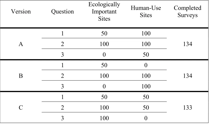
Table 3.1 Combinations of Ecological and Human-Use Sites Used in
Valuation Questions... 25
Table 3.2 Summary of Responses to Certainty Follow-Up Question... 29
Table 3.3 Summary of Responses to Zero-Bid Follow-Up Question…... 31
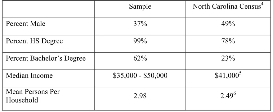
Table 3.4 Demographic Comparison Between Sample and Population... 33
Table 4.1 Summary of Sample Demographic Data……….... 41
Table 4.2 Response Intervals and Midpoints Used in OLS Estimation... 45
Table 4.3 OLS Results for the Linear and Semi-Log Functional Forms... 46
Table 4.4 MLE Results for the Linear and Semi-Log Functional Forms... 48
Table 4.5 Gibbs Sampler Results for the Linear Functional Form... 56
Table 4.6 Gibbs Sampler Results for the Semi-Log Functional Form... 57
Table 4.7 Gibbs Sampler Results for the Unique Elements of Σ... 63
Table 5.1 Candidate Intrinsic Growth Parameters for HWA... 85
Table 5.3 Candidate Values for the HWA-Hemlock Predation
Parameter... 89 Table 5.4 Reduction in HWA Infestation after Five Months of
Simulated Biological Control... 92 Table 5.5 Candidate Insecticide Decay Parameters and Years to 10%
Effectiveness... 93 Table 5.6 Biological Parameter Values... 94
Table 5.7 Gibbs Sampler Results for Multiple-Equation Semi-Log
Model... 96 Table 5.8 Net Present Value of Utility Losses... 103
Table 5.9 Summary of Posterior Distribution of the NPV of the Proposed
LIST OF FIGURES
Figure 2.1 Map of Documented Hemlock Woolly Adelgid Infestations... 10
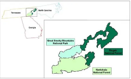
Figure 2.2 Map of the Study Area... 15
Figure 4.1 Points Where Marginal WTP for Ecological Protection is Positive... 60
Figure 4.2 Points Where Marginal WTP for Human-Use Protection is Positive... 60
Figure 4.3 Posterior Distribution of Expected WTP for Protecting 50 Ecological Sites and 75 Human Use Sites... 62
Figure 4.4 Postpredictive Specification Analysis Using Exact Intervals... 65
Figure 4.5 Postpredictive Specification Analysis Using Exact and Adjacent Intervals... 67
Figure 4.6 Marginal Willingness-to-Pay Surfaces... 70
Figure 4.7 Expansion Path for Optimal Control Network and Budget Constraint... 71
Figure 5.1 Hemlock Health and HWA Infestation in the Two-Species Simulation... 91
Figure 5.2 Simulated Baseline Conditions in the Treatment Network... 105
Figure 5.3 Ecological Site State Variable Values under Mitigation... 107
Figure 5.4 Human-Use Site State Variable Values under Mitigation... 107
CHAPTER 1
The tightening of public funds and the growing list of natural resource damages in the
United States and elsewhere highlight the need for efficient allocation of conservation
resources. The standard model for evaluating conservation projects in the US favors
strategies that maximize the number of protected units within the allocated budget.
Government conservation efforts such as the Environmental Quality Incentive Program
(EQIP), the Conservation Reserve Program (CRP), and the Wildlife Habitat Incentive
Program (WHIP) use the number of acres enrolled or the number of endangered species
represented to evaluate individual projects. Wu and Boggess (1999) show that using such
resource conservation criteria rather than maximizing economic benefits can lead to
highly inefficient allocations of conservation funds. In fact, maximizing the number of
protected units subject to a budget constraint assumes that benefits are linearly increasing
in these units. In reality, benefit functions can be highly nonlinear and may even reach a
maximum before the budget constraint becomes binding. Consider a predator
reintroduction program; without citing empirical evidence, I can safely say that the
marginal benefit of introducing grizzly bears or gray wolves becomes negative as their
populations conflict with human activities.
The reason resource conservation is a more popular means of program evaluation
is that economic benefits from ecosystem services can be difficult and costly to estimate.
Rarely do ecosystems provide strictly market-valued goods and services. Even with data
from a nonmarket valuation study to estimate benefits from ecosystem services, a static
impact on ecosystem services in future periods, thus affecting their marginal value and
changing the optimal policy response. To accurately evaluate environmental policy, a
dynamic model of the affected ecosystem may be required. Massey et al. (2006) combine
a dynamic population model and a recreation demand model to value changes in water
quality for the Atlantic Coast summer flounder fishery. There are very few examples of
studies that combine the empirical estimation of nonmarket benefits with a dynamic
model of environmental policy. I suspect this void is related to the difficulty of linking
the environmental good valued by the study to the policy outcome. For example, the
recreation demand study referenced by Massey et al. provides a marginal value for
increasing angler catch rates. The dynamic policy model only provides changes in fish
population. Linking the number of fish caught to the number of fish in the water is a
difficult task. Massey et al. address this with a third statistical model of angler catch to
link the recreation demand model and the dynamic policy model. What is unique about
the current work is that the nonmarket valuation project and bioeconomic model were
developed simultaneously. The result is a model that requires only a few reasonable
assumptions to link the empirically estimated benefit function to the dynamic model of
environmental policy.
Dynamic policy analyses such as Massey et al. can be used to allocate funds
among competing conservation projects but funding must also be allocated within a
project. In the current work I address both decisions. I develop a bioeconomic model to
damages caused by a destructive invasive insect on three federal lands in western North
Carolina. In addition to the dichotomous decision of whether or not to fund the project, I
address the issue of how the proposed policy allocates funds to protect two types of
forested sites with two different control media. The forest service has designated a
network of treatment sites over the 1.9 million acres of Great Smoky Mountains National
Park, Pisgah National Forest and Nantahala National Forest. Treatment sites were chosen
because they provide either ecological or human-use services. Each site will receive
chemical treatments, releases of a biological control agent, or both. The bioeconomic
model allows me to reallocate conservation resources and observe the effect on the net
present value (NPV) of the modified policy. While the current work does not solve for
an optimal mitigation strategy, this is the most immediate extension for this line of
research and the models presented here are developed to facilitate a dynamic optimization
routine.
The hemlock woolly adelgid (HWA) is an invasive insect that is quickly killing
hemlock trees in the northeastern United States. Chapter 2 provides background on the
introduction of the pest, the extent of the damages, and what types of control measures
are available to resource managers. This particular project is primarily concerned with
mitigating damages to public lands. Other studies have estimated the effects of HWA
infestations to private land values (Holmes et al, 2005); however, the policy examined
To estimate benefits from various mitigation strategies I have worked with US
Forest Service researchers to design and administer a contingent valuation (CV) survey.
The survey asks each respondent three valuation questions using a payment card response
format. This particular design produces data with latent willingness to pay (WTP) values
and a covariance structure in which an individual’s three valuation responses may be
correlated. I have developed a Bayesian estimation routine that explicitly addresses the
latency and covariance structure associated with this data generating process. Chapter 3
estimates a benefit function via ordinary least squares (OLS), maximum likelihood
estimation (MLE), and Gibbs sampling with data augmentation. The form of the benefit
function allows me to isolate the contributions of ecological and human use services as
well as their interaction to total benefits. This becomes an important feature of the policy
analysis.
The intertemporal properties of hemlock ecosystems, HWA infestations, and the
control media must be accounted for in the evaluation of the proposed mitigation
strategy. Chapter 5 combines the empirically estimated benefit function, actual costs of
control, and a dynamic biological model to form a bioeconomic model of mitigation
effort. The foundation of the biological model is a three-species predator-prey model
representing the interaction among forest health, the invasive species, and the biological
control agents. A fourth differential equation and state variable are added to the system
to represent the lasting effect of chemical control. A considerable challenge in specifying
biological variables interact. In most cases actual observations from the field are used to
find values for these parameters. Another task in specifying a dynamic model of
environmental policy is to determine how policy parameters enter the state equations and
what values they will take over the planning horizon. Forest Service and Park Service
documents provide the information necessary to characterize the proposed policy in terms
of the model. A computer simulation of the bioeconomic model finds that the proposed
policy has a positive NPV and is thus worthy of funding. Having addressed the
dichotomous question of whether or not to fund this particular policy the model can be
used to test if changes to the strategy, such as shifting resources from some treatment
sites to others or altering the mix of chemical and biological control, have a positive
impact on NPV.
Chapter 6 concludes with key findings and possibilities for future research. The
findings presented in this document offer contributions to several areas of environmental
and natural resource economics. The CV valuation survey addresses several emerging
design issues. The Bayesian estimation routine developed here is a rigorous approach to
a data structure that is fairly common in CV studies. Using empirical benefit estimates
for nonmarket environmental goods in a bioeconomic model is a recent development in
the literature and adding to the few studies that exist reveals new results and areas for
future research. One of those areas is dynamic optimization of the bioeconomic model.
The bioeconomic model developed here for policy simulation and evaluation can also be
optimal policy. I have made considerable progress in this direction, though no results are
CHAPTER 2
I. Infestation History
The hemlock woolly adelgid (HWA) is an insect native to Asia where it is a common but
largely harmless parasite of several hemlock species. In the early twentieth century
HWA was accidentally introduced to the western United States where it infested western
hemlock (Tsuga heterophylla). Like the Asian species, western hemlocks are mostly
unaffected by HWA infestations. However, by 1950 HWA had been introduced to
hemlock forests in the eastern United States. Hemlock species found in eastern forests
are more susceptible to HWA infestations. Since the discovery of HWA in Richmond,
Virginia the lack of natural predators has allowed infestations to spread rapidly.
Infestations have now been found in 15 eastern states. It can take as few as four years for
HWA to kill a mature hemlock, though some have survived infestation for a decade or
more (McClure et al, 2003). In the absence of an aggressive mitigation strategy we can
expect a 90% loss of hemlock resources in the eastern United States over the next 20
years (Jacobs, 2005).
Eastern hemlocks (Tsuga canadensis) are slow-growing, long-lived evergreens
that reach 60 to 70 feet in height and may live for 800 years or more. The geographical
range of eastern hemlock includes parts of Canada, extends from the east coast of the
United States westward to the Great Lakes region and as far south as Georgia. The
Carolina hemlock (Tsuga caroliniana) is a rare species that can only be found on the
HWA. Figure 2.1 shows the native range of eastern and Carolina hemlocks and counties
where infestations have been recorded1.
Figure 2.1 Map of Documented Hemlock Woolly Adelgid Infestations
II. Biology
Hemlock woolly adelgid have a complex life cycle that produces three generations per
year (McClure et al, 2003). One generation is capable of flight but is not able to
reproduce in North America for lack of a suitable spruce species they require for egg
deposit. The two generations that make up the reproducing population of HWA in North
America spread by “hitchhiking” and are carried by wind, birds, deer, and humans.
Twice each year they produce a single white cottony ovisac containing up to 300 eggs.
The ovisacs are very apparent and are the easiest way to identify an infestation.
After hatching, HWA settle at the intersection of a hemlock needle and its stem
and insert a long mouthpart through which they draw nutrients from reserves in the plant
tissue. Feeding by the HWA causes defoliation of infested branches, usually within a few
months. Dieback of major limbs can occur in a few years and progresses from the
bottom of the tree upward. Many trees die within four years while some are able to
survive longer with sparse foliage at the top of the crown. Very few weakened trees
recover and the factors that contribute to recovery are not well understood (McClure et
al, 2003).
III. Hemlock Resources
Historically, eastern hemlocks were found in about 20% of upland forest ecosystems in
their geographic range but this has been reduced to less than 6% by harvesting practices
and land use over the past century (McClure et al, 2003). Despite no longer being an
abundant component of eastern forest ecosystems, the eastern hemlock occupies an
Brook trout, an important game species, are found more commonly in streams
bordered by hemlocks where the shade of their dense foliage keeps water temperatures
cooler and their root systems prevent erosion of steep banks (Jacobs, 2005). Studies from
the Delaware Water Gap Recreation Area found that brook trout are three times as likely
to occur in streams bordered by hemlock than hardwood bordered streams (Ross et al,
2003). The implication is that a widespread loss of hemlocks could result in the loss of
ecologically and recreationally important species such as the brook trout.
A more immediate impact and one that affects a larger human population is that
which hemlock destruction has on aesthetic values and recreation experiences. Hemlocks
are an exceptional component of the natural scenery in mountain ranges along the east
coast. In addition to providing a scenic background at outdoor recreation areas and along
roads they provide shade at picnic areas, camp sites, and along hiking trails. It is
important to remember that areas affected by HWA infestation will not simply lose
hemlocks but that healthy hemlock stands will be replaced with standing dead trees for a
number of years. This will significantly reduce aesthetic values, increase the risk of
forest fires, and cause some recreation areas to close temporarily while dead trees are
IV. Control Options
The Forest Service and Park Service are currently using three methods of control on
federal lands to mitigate the impacts of HWA infestation and slow its movement to
non-infested areas. Insecticidal soaps and horticultural oils can be sprayed on hemlocks when
the objective is immediate knockdown of an insect pest. The soaps and oils act by
smothering all invertebrates on the tree at the time of treatment but there is no lasting
effect so trees can be reinfested immediately. Spraying requires large pieces of
equipment that are typically mounted on a truck, so this method is not practical for trees
more than 50 feet from a road. As such, this form of control is not a viable option for the
vast majority of hemlocks on public lands.
A second form of control is the use of a systemic insecticide. This is a chemical
that is injected into the soil at the base of the tree where the root system draws the
insecticide into the plant tissue of the stems and branches where the HWA feed. This
form of control will only kill organisms that are feeding on the tree and will prevent
reinfestation for three to five years after application.
The Forest Service and Park Service are also using a biological agent to control
HWA. A number of predatory beetles found in the native range of HWA have been
collected and observed in laboratory settings to assess their potential for biocontrol. Of
the many species that were collected a few exhibit the potential to be effective control
found to be a very effective predator of HWA (Cheah et al, 2004). Field studies have
shown that S. tsugae can reproduce after release, disperse locally, survive heat waves,
overwinter, and establish in a variety of different hemlock habitats (Cheah and McClure
2000). It responds well to laboratory mass rearing on HWA-infested foliage collected
from the field between fall and mid-summer. Field releases of S. tsugae began in
Connecticut in 1995 and elsewhere in 1999. Since 1995, over one-million S. tsugae have
been released on more than 100 sites in 15 eastern states, from South Carolina to Maine.
V. The Study Area
The purpose of this study is to estimate benefits from hemlock services and evaluate
proposed mitigation plans on three federal lands in western North Carolina and eastern
Tennessee. The three lands, shown in Figure 2.2, are Pisgah National Forest, Nantahala
National Forest, and Great Smoky Mountains National Park.
Great Smoky Mountains National Park straddles the North Carolina-Tennessee
border and covers nearly 521,100 acres. It is by far the most visited national park with
over 9 million visits in 2006, more than doubling the number of visits to the second most
visited park, the Grand Canyon. The Park hosts nearly one half-million camper-nights
and 400,000 hikers annually, many of whom hike part of the 70 miles of the Appalachian
Trail that runs through the park (National Park Service). Pisgah and Nantahala National
received approximately 6 million visits in 2006 (US Forest Servicea). Out of the nearly 2
million acres of the combined study area 32,000 are hemlock-dominated forest with
6,200 acres being old-growth hemlock stands.
Figure 2.2 Map of the Study Area
Infestations have been recorded throughout the study area and extensive damage
is already apparent at many popular recreation sites. At the time of writing, a mitigation
strategy is being implemented on all three lands in the study area. While it is not possible
to save all or even most of the hemlocks in the study area, a network of high-priority sites
has been identified and is receiving chemical, biological, or a combination of both
value or high human-use value. Ecologically important sites were identified from either
the North Carolina Natural Heritage Database or the Southern Appalachian Vegetation
Database (Jacobs, 2005). Sites that include native brook trout waters, provide habitat for
rare species, and are viable in the long term received preference in designating the
treatment network. Sites of high human-use value typically have a long history of
CHAPTER 3
I. Valuation of Hemlock Decline
The US Forest Service is conducting a study that will provide guidance to public forest
managers regarding the value of ecosystem services supplied by hemlock forests on the
land that they manage. The project, titled Valuation of Hemlock Decline on Public
Forests in the Southern Appalachian Mountains, will include a nonmarket valuation
(NMV) study of hemlock services in Pisgah National Forest, Nantahala National Forest,
and Great Smoky Mountains National Park. The data analyzed in the current work were
collected during a second pretest of the NMV survey that is being developed by Tom
Holmes2, Kathleen Bell3, and me. Four-hundred and one North Carolina residents
completed the survey. At the time of writing, the pretest results are guiding the
development of the full-scale survey. The full-scale survey will sample 1,500 people
within a 500 mile radius of Asheville, North Carolina and will differ in some respects
from the pretest phase of the survey. This chapter will deal primarily with the design of
the pretest version of the survey as it is these data that are analyzed in subsequent
chapters.
II. The Valuation Question
Survey respondents answered questions about their outdoor recreating behavior,
attitude toward the available control methods, and the importance of protecting hemlocks
in different areas before they reach the valuation questions. However, since the chapters
that follow are primarily concerned with estimating and applying a benefit function for
hemlock services, this chapter will focus on the development of the valuation questions.
It should also be noted that Kevin Boyle’s chapter in A Primer on Nonmarket Valuation
(2003), titled “Contingent Valuation in Practice,” was a valuable resource in designing
the survey though that may not be apparent from individual citations.
(A) The Good Being Valued
In designing a NMV survey intended to inform policy action, the first order of business is
to define the good that will be provided by the referenced policy. Thus far I have only
referred to ‘valuing a decline in hemlock health.’ A more specific, policy-relevant
definition is required for valuation. In particular, the proposed policy will maintain a
higher level of hemlock ecosystem services relative to a scenario in which no mitigation
action is taken. The baseline loss of hemlock services in the study area is severe. The
Environmental Assessment for Suppression of Hemlock Woolly Adelgid Infestations
(Jacobs [2005], henceforth ‘the Environmental Assessment’) estimates a 90% loss of
eastern hemlock resources and virtual extinction of Carolina hemlocks in the study area
over the next two decades. The mitigation strategy proposed by the Forest Service will
lessen the impact of HWA infestations relative to this baseline. The good being valued is
the difference between the loss of hemlock services under baseline conditions and that
which is lost once the mitigation strategy is in place.
Polasky et al. (2001) modeled heterogeneity in land prices when developing a
efficiency of limited conservation resources. I allow for heterogeneity of benefits over
the treatment network to examine the site selection problem in a similar way. The
mitigation strategy described in the Environmental Assessment specifies a network of
125-acre sites that will receive direct treatment for HWA infestation, to the exclusion of
all other hemlock stands in the study area. Each site is designated as either ecologically
important or culturally important. Throughout this document culturally important sites
are alternatively referred to as human-use sites. The specific characteristics of each type
of site are explained in Chapter 2, Section V. Resource managers will have to make
decisions regarding the allocation of conservation resources across sites. The relative
value of an additional ecological site as opposed to an additional human-use site can
guide efficient allocation of conservation resources over a treatment network.
Maintaining the distinction between the two types of hemlock services in the valuation
allows me to estimate a benefit function that isolates the marginal value of each type of
site.
(B) Valuation Approach
Given the severity of damage to hemlock resources and one of the affected areas being
the nation’s most popular national park, nonuse values are likely to be a substantial
fraction of total willingness to pay (WTP) to mitigate damages. It is difficult, and in
many cases impossible, to estimate nonuse values using revealed preference methods of
nonmarket valuation. The complementary relation between observable market behavior
revealed preference methods may not be sufficiently met to allow their application
(Brown, 2003). So we are left to choose an appropriate stated preference method to
estimate the value of hemlock decline.
Choice experiment approaches to stated preference, such as conjoint analysis, ask
a respondent to choose among a number of alternatives each with its own set of attributes.
To value improved hemlock health at various combinations of ecological and human-use
sites, respondents may be asked to choose between two different treatment networks,
each with its own cost, and a third choice that provides no treatment and would cost them
nothing. Choosing levels of the attributes across treatment networks is simple enough;
the Environmental Assessment provides ample information to design realistic choices.
The challenge in designing a choice experiment in this phase of the survey is that we
have little sense of what people are willing to pay for various mitigation programs. A
poor choice of prices for our choice sets combined with a fairly small sample could result
in little information.
A contingent valuation (CV) approach may be better suited for the pretest sample
and does not necessarily require even general knowledge about people’s WTP for the
environmental good. A CV survey can provide data sufficient to estimate a benefit
function for policy analysis and guide the design of an attribute-based survey in the
full-scale implementation of the study. The merits and limitations of CV are well covered in
complete review). However, certain issues are relevant to the design of this particular
survey and will be discussed as necessary in the sections that follow.
(C) Response Format
To choose a contingent valuation response format is to choose a balance between
efficiency and precision. Response formats that yield the most information are more
often found to elicit biased responses while those that are touted as incentive compatible
provide far less information given the same sample size. Representing one side of this
spectrum is the open ended format which has been all but abandoned due to a number of
problems in implementation. First, respondents are faced with an unfamiliar choice.
Rather than responding to a given price for a particular good, as they would face in a
market setting, they are asked to state the maximum price they would be willing to pay
for a good that is also unfamiliar. There is also a tendency for respondents to provide
strategic bids by bidding unreasonably high for policies they support or bidding zero
when they object to the policy but not necessarily the good being valued.
On the other side of the spectrum is the single-bounded dichotomous choice
format. When combined with a referendum provision mechanism Carson et al. (2000)
show this format to be incentive compatible and to produce the most truthful responses.
This is not a uniformly supported view. Brown et al. (1996) found that both dichotomous
choice and open ended responses overstate WTP when compared to actual donations with
the dichotomous choice format producing the highest estimates. The finding that
over several studies (Boyle et al. [1996], Ready et al. [1996]). In addition to producing
inflated WTP estimates dichotomous choice provides relatively little information
compared to other response formats. A ‘yes’ or ‘no’ response to a single bid amount
provides the researcher with an interval for WTP that is bounded on one side only. Given
that we are working with a fairly small sample size (401 respondents) dichotomous
choice is not a practical format.
Response formats such as multiple-bounded dichotomous choice and payment
card offer some middle ground in the choice between efficiency and precision. These are
discrete choice methods that can provide smaller, bounded intervals for WTP.
Multiple-bounded dichotomous choice can be subject to anchoring bias. Respondents appear to
take the first amount as a signal to the good’s value and their bids are therefore
influenced by it. Alberini, Boyle, and Welsh (2003) demonstrated this tendency by
presenting some bids in ascending order and others in descending order. Respondents
presented with ascending bids had lower estimated WTP than did those presented with
descending bids. The payment card response format has many of the same characteristics
as multiple-bounded dichotomous choice but is not subject to anchoring bias because
respondents view all of the bids at once. One may expect the range and distribution of
amounts on a payment card to influence responses; however Rowe et al. (1996) found no
evidence of this as long as the distribution of payment card amounts was not truncated
literature regarding contingent valuation response formats we opted for a payment card
response.
(D) Multiple Valuation Questions on a Single Survey
Another way to address small sample size is to ask each respondent more than one
valuation question. It is possible to double or triple the number of data points available
for estimation without unduly increasing the burden placed on the respondent. This will
raise some econometric issues and these are covered in the next chapter. For now we
concern ourselves only with the effect multiple solicitations may have on the valuation
responses.
The primary concern with multiple solicitations is ordering effects. Several
studies have found that WTP distributions have a tendency to change from one valuation
question to the next, particularly for respondents who are less familiar with the good
being valued (Bateman and Langford [1997], Halvorsen [1996]). Boyle et al. (1993)
found no evidence of ordering effects among experienced whitewater rafters when
valuing trips to the Grand Canyon but WTP estimates for inexperienced respondents are
influenced by question order. This finding highlights the importance of a well designed
information section that familiarizes the respondent with the good being valued. So
again, we are faced with the tradeoff between efficiency and precision. It is possible to
improve model variance by asking multiple valuation questions of each respondent but
ordering effects may bias the results. In this case we chose to include three questions on
the information section and valuation questions themselves. Three versions of the survey
were administered giving us nine different valuation questions. The combinations of
ecological and human-use sites used on each survey are reported in Table 3.1.
Table 3.1 Combinations of Ecological and Human-Use Sites Used in Valuation Questions Version Question Ecologically Important Sites Human-Use Sites Completed Surveys A
1 50 100 134 2 100 100 3 0 50
B
1 50 0 134 2 100 100 3 0 100
C
1 50 50 133 2 100 50 3 100 0
(E) Information Section
The information component of a survey can be used to address several potential
weaknesses of contingent valuation studies and minimize the associated biases (Carson et
al, 2001). One criticism of contingent valuation is that respondents are sometimes asked
to value goods with which they are unfamiliar. An argument can be made that people
make market decisions based on similar amounts of information every day, but
being valued will add credibility to the study. We have designed the survey so that
respondents have read several pages of information and answered qualitative questions
about hemlock protection before they reach the contingent valuation section of the
survey. The CV section has its own page of information preceding the questions to
further familiarize the reader with the resource and the policy scenarios they will be
valuing.
Respondents should also believe the good can be provided as stated in the
question and that their responses will be used in the decision making process.
Throughout the survey respondents learn about the proposed mitigation strategy that is
referenced in the CV questions and are told that their responses will help guide forest
management decisions. In hindsight specific language to this effect should have been
included in the information section immediately preceding the CV questions. This
should be one of the improvements made to the full-scale survey. The reader can find the
one-page information section on page 17 of the survey which is included as an appendix.
The information section also prepares the reader for multiple valuation questions
and provides the payment vehicle. Respondents are told that it is not possible to protect
all of the hemlocks in the study area and only hemlocks in designated treatment sites will
receive protection. Respondents read about the two types of sites that are being
considered for treatment and that they will be presented with three different plans that
protect varying numbers of ecological and human-use sites. The mitigation program will
we would like to know how much they would be willing to pay to support each of the
three proposed programs. Having familiarized the respondent with the good being
valued, assured them that it will be provided as described, and that their responses will
guide management decisions we feel we have addressed the main CV criticisms. A more
specific description of exactly how participants’ responses will influence future decisions
should be included in the information section of the full-scale survey.
(F) Follow-Up Questions
Several contingent valuation surveys have asked participants to express how certain they
are about their responses. Champ et al. (1997) follow a dichotomous choice contingent
donation question by asking respondents to rate on a scale of one to ten how likely they
are to actually donate the amount they indicated. There was close correspondence
between the characteristics of those who were quite certain about their response to the
contingent donation question and the characteristics of those who actually did donate.
They also found that mean WTP for the most certain responses are not statistically
different from the mean amount of actual donations.
Welsh and Poe (1998) use a payment card response format and ask respondents to
choose from five levels of certainty, ranging from ‘definitely no’ to ‘definitely yes’, for
each bid amount. The resulting response format is a two-dimensional matrix with one
dimension representing WTP amounts and the other indicating the likelihood that the
respondent would pay the corresponding amount. They estimate three different models
sure’ as the payment threshold and compare the results with estimates from dichotomous
choice and payment card surveys. Their results support previous studies that find
dichotomous choice to produce the highest estimates - slightly higher than the ‘not sure’
model. This suggests that when faced with an amount respondents are not sure they
would be willing to pay in a dichotomous choice setting, they will respond in the
affirmative. As one might expect, the ‘definitely yes’ model produced the lowest
estimates.
We chose to include a single certainty follow-up question to our payment card
valuation question. Our goal was to take advantage of the payment card response format
and allow respondents to express uncertainty but reduce the burden placed on the
respondent relative to the Welsh and Poe study. This question format raises the issue of
estimation. Champ et al. (1997) estimate a typical dichotomous choice model but change
‘yes’ responses to ‘no’ if the level of certainty falls below a level chosen by the
researcher. Welsh and Poe (1998) estimate typical interval response models but change
the response interval according to the level of certainty they wish to allow. Neither of
these estimation approaches can be used for the data collected with payment card
response and single follow-up question. In fact, responses to the certainty follow-up
questions are not used at all in the estimation routine discussed in the next chapter.
However, a number of possibilities could be explored. One can simply discard
observations for which respondents indicated a level of certainty below some chosen
sample size is small to begin with. Alternatively, we can develop weighted maximum
likelihood estimation routine in which each observation’s contribution to the likelihood
function is assigned a weight that corresponds to the level of certainty expressed. These
and other approaches will be explored and used to determine if a single certainty
follow-up to a payment card valuation question is practical. A tabulation of certainty responses
for positive valuations are reported in Table 3.2.
Table 3.2 Summary of Responses to Certainty Follow-Up Question
Extremely Certain Somewhat Certain Not Certain
5 4 3 2 1
525 298 121 22 16
We also included a follow-up question to identify protest bids. Only people who
indicated they were not willing to pay any of the amounts on the payment card were
asked this question. The lowest amount on the payment card is $2 so a refusal to pay this
amount in increased annual taxes is interpreted as a zero-bid. The zero-bid follow-up
question is reproduced below.
You said you were not willing to pay any of the amounts listed above, please circle the response below that best describes the reason for this response. (Circle one response)
1 $0 IS WHAT IT WOULD BE WORTH TO ME
3 I CANNOT AFFORD TO PAY TO PROTECT FOREST QUALITY
4 I OBJECT TO THE QUESTION
5 NO NEW TAXES
6 OTHER: (please specify):_________________________
Only responses 1, 3, and in some cases 6 are considered legitimate zero-bids. Out
of 1203 responses 221 indicated they would not be willing to pay any of the listed
amounts to support the referenced mitigation plan. Table 3.3 tabulates the responses to
the zero-bid follow-up question. A disproportionate number of zero-bids were given in
response to questions in which one type of site received no treatment. On 268 of the
1203 valuation questions administered (about 22%) either ecologically important sites or
human-use sites received no treatment in the referenced mitigation strategy. But these
questions account for 91 of the 221 zero-bids (about 41%). Responses to the follow-up
question for which people chose ‘Other’ and provided their own reason support the
notion that many people reject strategies that exclude one type of site. The most common
open-ended response is that they will not support a plan that excludes one type of site
Table 3.3 Summary of Responses to Zero-Bid Follow-Up Question
$0 is what it would be worth to me
People should not have to pay
to protect forest quality I cannot afford to pay to protect forest quality
I object to the question
No new
taxes Other
18 33 58 15 39 58
III. Survey Administration
Consumer Insights Research, a marketing research firm based in Asheville, North
Carolina, was hired to administer the survey. This included a focus group pretest,
adapting a paper version of the survey to a web-based version, recruiting a sample for the
second pretest, and delivering the resulting data set. Consumer Insights Research
recruited fourteen adults to participate in one of two focus groups. Individuals were
screened and placed into the ‘environmentalist’ group or the ‘property rights’ group.
Separate focus groups were conducted to detect bias in the survey. The focus group
sessions were conducted in Asheville, North Carolina on October 12, 2005. Results of
the focus group were favorable. Only minor changes to language and formatting were
made and neither group detected any bias in the survey.
Web-based survey instruments have a number of practical advantages over other
survey modes. Once a sample is recruited there is virtually zero marginal cost to
collecting data. Marginal costs from administering paper or in-person surveys and then
cleaned and delivered almost immediately without the risk of human error associated
with data entry. A web based instrument ensures that respondents view components of
the survey in the order intended. It is also possible to collect information on how long the
respondent took to complete the survey or how much time they spent on individual
questions.
The obvious limitation of typical web-based surveys is that they are not
representative of the population. People without internet access are precluded from the
sample. In our case only 67 out of 4,144 people contacted (1.6%) could not participate
because they did not have internet access. It is likely that people who were excluded
from the sample for other reasons lacked internet access as well, but we do not have these
data. Table 3.4 compares the demographic profile of our sample with North Carolina
census data.
Females are overrepresented in our sample and respondents tend to have higher
education than the sample frame population. The survey only collected data on income
ranges but the median income in North Carolina falls within the median range reported
for the sample. Three-hundred and nineteen of the 401 survey respondents were recruited
over the phone. The balance of the sample received an email recruiting them to the
survey. The number emails sent is not available so it is not possible to calculate a
response rate for that portion of the survey. However, 4,144 people were contacted by
phone and deemed eligible for the survey, making the response rate for that portion of the
Table 3.4 Demographic Comparison Between Sample and Population
Sample North Carolina Census4
Percent Male 37% 49%
Percent HS Degree 99% 78%
Percent Bachelor’s Degree 62% 23%
Median Income $35,000 - $50,000 $41,0005
Mean Persons Per
Household 2.98 2.496
contacted over the phone actually completed the survey online. The low response rate
and lack of representativeness calls into question the web-based survey mode. The
full-scale survey will likely be administered using a more traditional survey mode that has
shown to produce better sampling results.
4 Census data refer to 2006 values unless otherwise noted 5 2004 census data
CHAPTER 4
I. Estimation Approach
This chapter develops a Bayesian estimation routine for interval response data that allows
for correlation among responses. The survey described in Chapter 3 produces a dataset
with two structural characteristics that must be addressed in estimation. The first is the
latent willingness-to-pay (WTP) values that result from the payment card response
format. When a contingent valuation survey employs a payment card response format,
the researcher will not observe point-values for WTP but rather intervals that contain the
respondents’ WTP. The highest amount to which the respondent answered in the
affirmative and the lowest amount the respondent refused provide bounds on WTP.
A number of estimation approaches have been used to address the interval nature
of payment card responses. Cameron and Huppert (1989) estimate payment card data via
ordinary least squares (OLS) and maximum likelihood (MLE) and show that the OLS
approach produces parameter estimates that are biased toward zero. The effect on
expected WTP is ambiguous because parameters with a negative sign are biased upward
while positive parameters are biased downward. I follow the approach taken by Cameron
and Huppert, estimating the model using both OLS and MLE and find strong evidence
for dampening bias in the OLS parameter estimates.
Fernandez et al. (2004) estimate interval contingent valuation data using a
Bayesian approach. The Bayesian estimation routine utilizes a data augmentation step to
data are then used as conditioning factors in a Gibbs sampler to characterize the joint
posterior distribution for the parameters of interest.
In addition to the interval nature of the responses, the survey’s multiple
solicitation design introduces the possibility of correlated responses. With 401 completed
surveys and three valuation responses on each survey the data contains 1203 observations
with which to estimate a model. However, it is likely that an individual’s responses are
correlated in which case the assumption of a strictly diagonal error covariance matrix
would not hold. Estimating the model as if all 1203 responses are independent would
result in inefficient parameter estimates and bias the standard errors. A multiple equation
model that estimates each survey participant’s set of responses as a system can
adequately address the covariance structure. The bias of OLS estimates and the
numerical difficulties associated with estimating a multiple-equation model via maximum
likelihood make the Bayesian approach an attractive choice for estimation. The model
developed by Fernandaz et al. is a single-equation model and is appropriate if responses
satisfy the independence assumption. Huang’s (2001) Bayesian SUR Tobit model of
censored consumption data establishes a multiple-equation framework that can
accommodate a general error structure. In this chapter Huang’s multiple-equation
approach is used to generalize Fernandez’s Bayesian estimation of interval data to
II. Modeling Assumptions
Consider a respondent who bids above the conditional mean on one of the three valuation
questions. We may classify this person as a “high bidder” and expect them to bid above
the conditional mean on the other two valuation questions as well. So a “high bidder”
will have a three-vector of errors for which every element is positive. Likewise there
may be “low bidders” in the sample for which all three elements of their error vector are
negative. The single equation models ignore this type of correlation and consequently
produce inefficient parameter estimates and biased variance estimates (Kennedy, 1992).
A multiple equation model that allows for correlation among an individual’s
responses but assumes independence across individuals will include one equation for
each of the three questions on a survey. The unknown parameters in the model are the
vector of coefficients in the regression equation and the covariance matrix that describes
how a respondent’s WTP responses are related to each other. The multiple-equation
model estimates this covariance matrix revealing the nature and magnitude of the
correlation among responses.
(A) The Data Generating Process
I assume that the data generating process behind the valuation responses is linear in
parameters so that,
where is the realization of the latent WTP value or some transformation thereof, is a
row-vector of coefficients, is a vector of values for the explanatory variables, is a
normally distributed error, i indexes individuals, and j indexes the questions on a survey.
Because the three responses from each individual may be correlated, the errors are best
described as a set of N three-vectors, each with a zero mean vector and three-by-three
covariance matrix Σ, so that ~ 0, Σ .
(B) The Likelihood Function
Assuming errors are distributed trivariate normal the likelihood function is expressed as
, Σ|X 1
2π ⁄ |Σ| /
exp 1
2 y x β Σ y x β dy dy dy ,
(4.2)
where X is the stacked data matrix, and denote the lower and upper bounds on
individual i’s stated WTP for the jth question, is a three-by-K matrix of data, and is a
realization of the latent three-by-one WTP vector for the three questions answered by
individual i. The likelihood functions used in both the maximum likelihood approach of
Cameron and Huppert (1989) and the Bayesian estimation used by Fernandez et al.
(2004) are products of one-dimensional integrals of conditional probability distribution
probability of a respondent choosing that interval conditional on the data. Taking the
product of these individual probabilities to arrive at a likelihood function assumes
independence across responses. When each person provides multiple responses this is no
longer a reasonable assumption. However, it is reasonable to assume that one
respondent’s set of answers are independent from that of another respondent. So the
appropriate likelihood function when each respondent is providing three answers will be
a product of three-dimensional integrals. Each three-dimensional integral represents the
probability of observing an individual’s set of three responses given the data. Taking the
product of these three-dimensional integrals over all N respondents provides a likelihood
function that allows for correlation within an individual’s responses but assumes
independence among individuals.
Estimation of this model via maximum likelihood requires evaluating the
three-dimensional integral in (4.2) for each iteration in an optimization routine. Computational
approaches such as quadrature can be used to approximate (4.2) but are subject to a
number of computational difficulties. One can ignore the correlation in an individual’s
set of responses and estimate a single equation model that assumes independence among
all responses. Two such models are estimated in Section III. Least-squares and
maximum likelihood estimation of the single equation model provide first
approximations and means for comparison with the multiple equation model. Another
Bayesian estimation via Gibbs sampling. Section IV presents the Bayesian estimation of
the multiple equation model.
(C) Form of the Willingness-to-Pay Function
The contingent valuation questions ask respondents what they are willing to pay to avoid
a reduction in environmental services. This characterization is consistent with the
Hicksian concept of compensating variation (Flores, 2003). Using that definition it is
possible to derive a WTP function from a utility function with desirable properties.
However, as is often the case in CV studies this exercise is constrained by data
availability (Cameron and Huppert, 1989) and, in this particular case, the focus on
dynamic policy analysis that will be covered in Chapter 5. The form of the WTP
function was chosen to answer the policy questions of interest, allow for testing of
bidding behavior that is consistent with economic theory, and facilitate the analytical
derivations required for dynamic analysis.
The WTP function used in the OLS, MLE, and Bayesian models is
·
2 5
(4.3)
Ecoij and Useij are the number of ecologically important sites and human-use sites
included in the treatment network for the jth question answered by individual i. WNC is a
dummy variable used to identify respondents that are residents of western North
five income categories the ith respondent indicated. Parameters on the income dummies
should be interpreted as intercept shifts relative to the lowest income category, which has
been omitted.
The natural occurrence of hemlocks in North Carolina, with very few exceptions,
is restricted to the western part of the state where elevation of the southern Appalachian
mountains keeps average temperatures lower. The dummy variable WNC is included in
the WTP function to capture an intercept shift for respondents who live closer to the
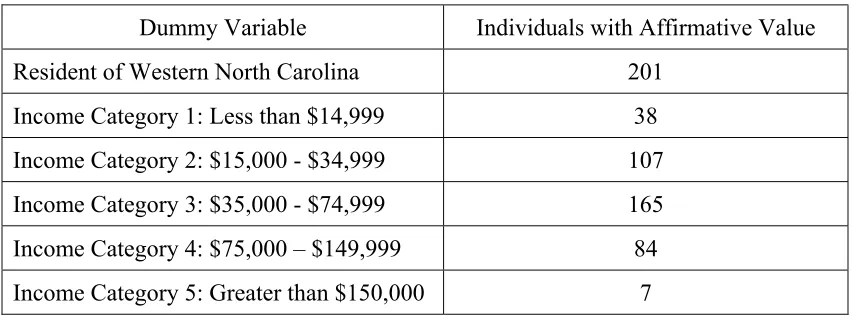
resource. Table 4.1 shows the number of sampled individuals who reside in western
North Carolina and those that indicated each of the five income categories.
Table 4.1 Summary of Sample Demographic Data
Dummy Variable Individuals with Affirmative Value
Resident of Western North Carolina 201
Income Category 1: Less than $14,999 38
Income Category 2: $15,000 - $34,999 107
Income Category 3: $35,000 - $74,999 165
Income Category 4: $75,000 – $149,999 84
Income Category 5: Greater than $150,000 7
The form of the WTP function allows a number of validity tests to assess the
survey design and the degree to which responses are consistent with economic theory.
One common test of validity is a scope test which, according to the NOAA Panel on
to the scope of provision (Arrow et al., 1993). Most applications of the scope test
consider a WTP function that is increasing in provision to exhibit adequate
responsiveness to provision (see Smith and Osborne [1996], Rollins and Lyke [1998],
Carson et al. [2001] for examples). A WTP function that is quadratic in the provision
variables allows a researcher to test for positive but diminishing marginal WTP - a scope
test of the second order. This would require the first partial derivatives with respect to
Eco and Use to be positive and the second partial derivatives to be negative. These
conditions are summarized by expressions (4.4) through (4.7).
2 0 (4.4)
2 0 (4.5)
2 0 (4.6)
2 0 (4.7)
for Eco and Use ,where the sets E and U represent the range of values for ecologically important and human-use sites referenced in the survey. A second test of
validity examines the relationship between expected WTP and income. A WTP function
0 . (4.8)
Two functional forms are estimated and compared. In the strictly linear
functional form, of equation (4.1) refers to the untransformed realization of the latent
WTP values. A semi-log functional form is also estimated in which the natural log of
WTP is regressed on a linear function of explanatory variables. The semi-log functional
form assumes a lognormal distribution for WTP and is commonly used in CV studies
because it imposes non-negativity on WTP and better fits the frequently skewed
distributions of CV responses (Cameron and Huppert, 1989).
III. Single-Equation Models
Reasons for estimating the less sophisticated single-equation models are severalfold.
First, the straightforward and widely understood mechanics of least-squares estimation
make the OLS estimates useful in establishing expectations of the maximum likelihood
and Bayesian estimates, which can be subject to computational difficulties such as failure
to converge and sensitivity to starting values. Second, using the OLS estimates as
starting values in the maximum likelihood and Gibbs sampling algorithms improves their
computational efficiency. Finally, the relative merits of each estimation approach can be
measured and weighed against the increased complexity of more sophisticated routines.
(A) Ordinary Least Squares Estimation of Interval Response Data
Estimating an interval response model using OLS requires choosing a point value to
distributed within the intervals any choice will be arbitrary. Cameron and Huppert
(1989) use the midpoint of each interval and that approach is maintained in this analysis.
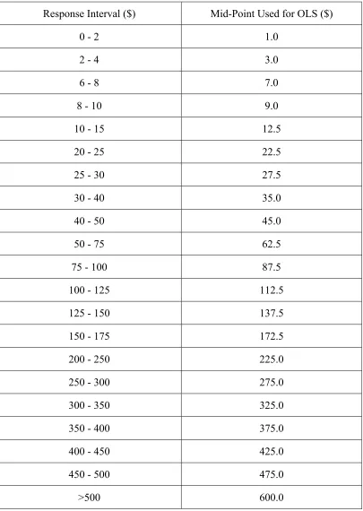
Table 4.2 shows the response intervals and corresponding midpoints used for estimating
the linear functional form. The semi-log functional form is estimated by taking the
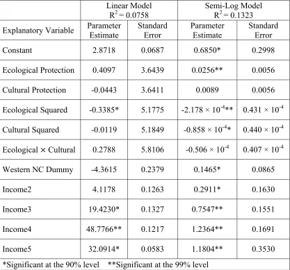
natural log of these midpoints and conducting OLS in the usual way. Table 4.3 reports
the results of OLS estimation. Least squares estimation of the data favors the semi-log
functional form. In contrast with the linear specification all parameter estimates have the
expected sign and the higher R-square measure indicates a lower model variance for the
semi-log model. Economic interpretation of individual parameter estimates is reserved
for discussion of the Bayesian results since the maintained assumption is that a
Table 4.2 Response Intervals and Midpoints Used in OLS Estimation
Response Interval ($) Mid-Point Used for OLS ($)
0 - 2 1.0
2 - 4 3.0
6 - 8 7.0
8 - 10 9.0
10 - 15 12.5
20 - 25 22.5
25 - 30 27.5
30 - 40 35.0
40 - 50 45.0
50 - 75 62.5
75 - 100 87.5
100 - 125 112.5
125 - 150 137.5
150 - 175 172.5
200 - 250 225.0
250 - 300 275.0
300 - 350 325.0
350 - 400 375.0
400 - 450 425.0
450 - 500 475.0
Table 4.3 OLS Results for the Linear and Semi-Log Functional Forms
Linear Model R2 = 0.0758
Semi-Log Model R2 = 0.1323 Explanatory Variable Parameter
Estimate
Standard Error
Parameter Estimate
Standard Error
Constant 2.8718 0.0687 0.6850* 0.2998
Ecological Protection 0.4097 3.6439 0.0256** 0.0056
Cultural Protection -0.0443 3.6411 0.0089 0.0056
Ecological Squared -0.3385* 5.1775 -2.178 × 10⁻⁴** 0.431 × 10⁻⁴
Cultural Squared -0.0119 5.1849 -0.858 × 10-4* 0.440 × 10-4
Ecological Cultural 0.2788 5.8106 -0.506 × 10⁻⁴ 0.407 × 10⁻⁴
Western NC Dummy -4.3615 0.2379 0.1465* 0.0865
Income2 4.1178 0.1263 0.2911* 0.1630
Income3 19.4230* 0.1327 0.7547** 0.1551
Income4 48.7766** 0.1217 1.2364** 0.1691
Income5 32.0914* 0.0583 1.1804** 0.3530
(B) Maximum Likelihood Estimation of Interval Response Data
Assuming all errors are independent and identically distributed implies Σ from equation (4.2) will be a strictly diagonal matrix with identical elements along the diagonal. This
reduces the three dimensional integral in (4.2) to a product of three one-dimensional
integrals. Thus the likelihood function becomes
, Σ|X 1
√2 exp 2 , (4.9)
for i = 1…N, j = 1…3. Furthermore, we can appeal to the First Fundamental Theorem of
Calculus to express the integral over the normal probability density function as a
difference between two normal cumulative distribution functions
, Σ|X Φ Φ . (4.10)
Using this form of the likelihood function in an optimization routine reduces the
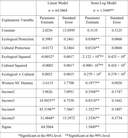
computational burden relative to evaluating (4.9). Maximum likelihood results for the
single-equation model are presented in Table 4.4.
The likelihood function (4.10) can be used to estimate the linear and semi-log
functional forms. To estimate the semi-log model the bounds on the intervals are logged
and the likelihood function is maximized in the same way. As in least squares estimation
Table 4.4 MLE Results for the Linear and Semi-Log Functional Forms
Linear Model
64.5064
Semi-Log Model
1.5449**
Explanatory Variable Parameter Estimate Standard Error Parameter Estimate Standard Error
Constant 2.0256 13.0595 0.3135 0.3125
Ecological Protection 0.3985 0.2461 0.0308** 0.0060
Cultural Protection -0.0172 0.2464 0.0124** 0.0060
Ecological Squared -0.0032* 0.0017 -2.122 × 10⁴** 0.425 × 10⁴
Cultural Squared -0.0002 0.0017 -0.900× 10⁴** 0.424 × 10⁴
Ecological Cultural 0.0025 0.0015 0.279 × 10⁴ 0.379 × 10⁴
Western NC Dummy -3.6115 3.7708 0.1977** 0.0920
Income2 3.9626 7.0951 0.3568** 0.1747
Income3 18.9435** 6.7538 0.8318** 0.1662
Income4 45.3196** 7.3667 1.3527** 0.1807
Income5 31.4848* 15.3972 1.3536** 0.3734
Sigma 64.5064 1.5449**
*Significant at the 90% level **Significant at the 99% level
from the semi-log model are statistically significant and their algebraic signs are
consistent with expectations. Specifically, protection of human-use sites and being a