The Smart Agent-based Model in Urban Growth Problems.

(1)

ABSTRACT

ZHANG, QIANG. The Smart Agent-based Model in Urban Growth Problems. (Under the direction of Dr. Raju Vatsavai).

As per United Nations (UN) projections, it is expected that another 2.5 billion will be

added to the urban populations by 2050. Urban growth models were widely employed to

study urban expansion. In this study, we present a framework for the integration of an

agent-based model (ABM) with the popular cellular automata (CA) based FUTure

Urban-Regional Environment (FUTURES) model. This thesis addresses one of the key challenges

in urban growth modeling, which is to capture the communication and behavior of agents

in order to infer the agent’s intent to develop a land parcel. With the interaction between

agent-based model and urban growth model, we simulated the decision-making process

of landowners when dealing with the urban development.

Many existing agent-based model frameworks were implemented using traditional

shared and distributed memory programming models. On the other hand, recent Apache

Spark is becoming a popular platform for distributed big data in-memory analytic. This

thesis presents an implementation of agent-based sub-model in Apache Spark framework.

With the in-memory computation, Spark implementation outperforms the traditional

distributed memory implementation using MPI. This report provides (i) an overview of

our framework capable of running urban growth simulations at a fine resolution of

30-meter grid cells, (ii) a scalable approach using Apache Spark to implement an agent-based

model for simulating human decisions, and (iii) the comparative analysis of performance

(2)

(3)

The Smart Agent-based Model in Urban Growth Problems

by Qiang Zhang

A thesis submitted to the Graduate Faculty of North Carolina State University

in partial fulfillment of the requirements for the Degree of

Master of Science

Computer Science

Raleigh, North Carolina

2019

APPROVED BY:

Dr. Munindar P. Singh Dr. Steffen Heber

(4)

DEDICATION

This is dedicated to my grandparents, Shuxiang Jiang and Jinyi Kang, who believe in me

and inspire me, who love me and have supported me every step of the way.

"Cross the Bridge when you get to it, in the end things will mend." Without their comfort, I

(5)

BIOGRAPHY

Qiang Zhang received his bachelor’s degree in telecom engineering in University of Science

and Technology Beijing. After graduation, he joined a mobile security company and had

been working as malware analyst for 3 years. He attended North Carolina State University

in 2013, joining STAC Lab under the advice and Dr. Raju.

His thesis projects were focused on Agent-based model and high performance

(6)

ACKNOWLEDGEMENTS

I would like to express my sincere, heartfelt thanks to my supervisor, Dr. Raju Vatsavai, for

introducing me to the fantastic world of Geospatial Sciences, continually guiding me and

giving me his invaluable advice, constant encouragement and precise modification on this

road.

Besides my advisor, I would like to thank Center of Geospatial Analytics, for their

in-sightful help and guidance of this work.

And also, my sincere appreciation to all of my friends, especially Ziqi Diao, M.J Mu and

Binyuan Wu whom friendly encourage me in writing the thesis. When time gets tough, I

(7)

LIST OF TABLES

Table 2.1 Model Comparison . . . 7

Table 2.2 Comparison of median value of land (per sqrt feet) value distribution before and after the interpolation . . . 19

Table 2.3 Neighborhood Influence for multi-label approach . . . 24

Table 2.4 Logistic Regression result . . . 28

Table 2.5 CART result . . . 28

Table 2.6 SVM result . . . 29

Table 2.7 Bayesian Network result . . . 29

Table 2.8 Random Forest result . . . 30

Table 2.9 Simulation Result without Neighborhood Influence . . . 31

Table 2.10 Simulation Result with Neighborhood Influence . . . 31

Table 2.11 Simulation Result with Neighborhood Influence and Bargain . . . 32

Table 3.1 Computation Time for Different Core Number with the FLAME Frame-work . . . 54

(10)

LIST OF FIGURES

Figure 2.1 Cabarrus County, NC, USA . . . 10

Figure 2.2 The communication between ABM and CA in each time step . . . 12

Figure 2.3 The FUTURES land change modeling framework[Mee13] . . . 14

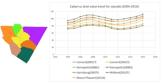
Figure 2.4 Cabarrus land value trend for zip code (2004-2006) . . . 19

Figure 2.5 Agent-based model conceptualization . . . 22

Figure 2.6 Allocation agreement illustration . . . 26

Figure 2.7 Willingness agreement illustration . . . 27

Figure 2.8 Prediction accuracy with land value increase rate change . . . 30

Figure 2.9 Error propagation observation . . . 33

Figure 3.1 Example of landscape cell, landscape parcel and parcel neighborhood 36 Figure 3.2 Communication between Urban Growth Simulator and Human In-volvement Simulator for Rounds . . . 37

Figure 3.3 Human involvement module communicates with urban growth model 38 Figure 3.4 Working flow of urban growth model and human involvement simu-lating module for one-time step . . . 40

Figure 3.5 The logic flow of the FLAME . . . 49

Figure 3.6 Flow illustration when implementing with the FLAME . . . 50

(11)

CHAPTER

1 INTRODUCTION

In recent years, some UGMs have simulated the urban growth tendency. However, some of

the work focuses on only one driver of urbanization[PF08] [Rom99] [KC03]. We believe that a realistic model of urban growth needs multiple driving factors and a means of modeling

interactions between individual stakeholders in order to address the social factors involved

in urbanization.

To achieve this goal of simulating urban growth to predict the area of urban

develop-ment, agent-based models (ABM) could provide such advantages to present and model the

urbanization growth with the multiple factors as economic status, individual

(12)

bottom up where all the individual computational elements are designated as an agent.

The behavior of the system can be integrated from micro-level interactions of the agents.

ABMs are widely used in various application domains, including but not limited to, biology,

economy, psychology and crowd behavior studies. Simulations with ABM can obtain not

only the result of the whole simulating system but also the snapshot of each agent in the

system, which could help us understand the underlying relationships of the system further.

An agent-based model seeks to simulate the complex global behaviors via the most

atomic units: individual, autonomous decision makers known as agents. The micro-level

decisions involved in modeling agents manifest themselves globally in the aggregate

be-havior of the individual agents. We view this perspective as a natural way of modeling both

the individual development decisions and the social factors involved. Besides, simulations

involving ABMs allow aggregate behavior to be understood at any level of granularity since

the underlying drivers are happening at the lowest level and not from the "top down."

However, with the explosive growth of data involved in the simulation, more and more

computational resources are required, especially in the geospatial application domain. In

this paper, we build an ABM to simulate the decision-making procedure of the landowners

in urban growth problems.

Our central goal in this work is to develop a discrete time-stepped intelligent agent model

that couples urban growth with individual stakeholder decisions and takes demographic,

economic and geographic information into account as driving factors. In addition, we

also seek to demonstrate the application of machine learning algorithms in the modeling

process. In our ABM design, we fully consider and conceptualize the possible principal

elements that may affect the landowners’ decisions in urban development. For a more

accurate simulation, we use not merely the landowner’s properties as computation input,

(13)

into account as well. All the core characters are shaped into heterogeneous agents. In order

to compare the computation performance, our module is built with both Apache Spark and

a generic agent-based modeling platform, the FLAME, which supports message passing

interface (MPI) and can be executed on multiple hardware and software platforms.

We make the following specific contributions:

• We implemented an ABM based on Apache Spark, which dramatically accelerates

the simulation speed compared to the prevailing ABM framework the FLAME.

• We couple an ABM with a cellular automata (CA) model (FUTURES). The interaction

between the two modules facilitates the ability of stakeholders to detect and analyze

the change of the conditions. By doing this, we reduce the error propagation with

better initial predictions.

• We implement an ABM to simulate the decision-making process in the urban growth

process. Also, each agent in the system is given the ability to make an intelligent and

more accurate decision by analyzing and understanding the historical urban growth

patterns from the data over time.

• We specify a multi-level decision hierarchy instead of outputting yes/no decision for the stakeholders. Such design enhances the ability of stakeholders to make more

flexible and intelligent decisions.

• We add a bargaining process in the urban development process between

landown-ers and developlandown-ers. Our results indicate that this strategy could better capture the

stakeholders’ behavior and conduct a more realistic simulation.

This thesis is mainly divided into two parts. In the first parts, we integrate the smart

(14)

improve the model with more accurate prediction. And the second part covers an approach

to make the urban growth simulation model execute faster by implementing Agent-based

(15)

CHAPTER

2 SAMRT AGENTS IN URBAN GROWTH

SIMULATION

2.1 Related Work

CA models are used to represent the urban and regional growth along with many other

technologies.[Ars13]proposed a hybrid model consisting logistic regression model, Markov chain (MC) and Cellular automaton (CA) to enhance the performance of traditional urban

(16)

urban growth trend of various land use classes. And[Fen16]also came up with a refined CA model which integrated partial least square regression (PLS-CA) and geographical

informa-tion systems (GIS). The introducinforma-tion of new algorithms and technologies could improve the

accuracy of the urban growth prediction, but in some circumstances, people would like to

understand the process of urbanization in a micro-level simulation. The urban growth and

neighborhood influence were estimated through calibrated parameters, which reflect only

the landscape features implicitly[CG98] [Cla97] [Cou97] [Bat07]. As a bottom-up model, CA cannot represent well macro-scale political, economic and cultural driving forces that

influence urban growth[War00] [MS00]and[CH89]argued that the local economy has a significant impact on the urban growth, specifically mentioned the house price and land

market.

Some existing CA models could be used to predict urban growth. While there are many

similarities among the models, each still differs in its modeling framework and assumptions,

as well as specific algorithms used to determine urban growth. So broadly these models

can be categorized into deterministic and stochastic. GEOMOD[Hal95] [PJ01]is a relatively simple deterministic model, it needs the input as spatial data representing observed land

cover, a site suitability surface, and an estimation of the quantity of cells to be developed.

Here the site suitability is calculated through a regression function with the parameter

of a pile of different layers of data. GEOMOD uses the optimization algorithm to select

the most suitable location. SLEUTH[Cla97]is a much more complex deterministic model, and it is widely used through the United States, the input it requires are historical urban

growth, road construction and slope along with an exclusion layer that acclaims what

cells cannot be developed. LCM (Land Change Modeler)[Eas09]is a stochastic model, it has three modules: change analysis module to determine the quantity of cells to be

(17)

site suitability surface for new development, and change predictions that allocate new cells

based on the site suitability surface. And FUTURES (FUTure Urban-Regional Environment

Simulation) has three core components as Site Suitability, Per capita demand and Patch

growth algorithm (PGA), And we use FUTURES as our CA model in our study, we will

introduce more in later sections.

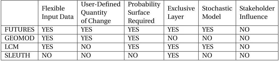
We did a comparison with these four models in Table 2.1.

Table 2.1Model Comparison

Flexible Input Data User-Defined Quantity of Change Probability Surface Required Exclusive Layer Stochastic Model Stakeholder Influence

FUTURES YES YES YES YES YES NO

GEOMOD YES YES YES NO NO NO

LCM YES NO YES YES YES NO

SLEUTH NO NO NO YES NO NO

We can see that the common limitation is that the ignorance of stakeholder activity in

the urbanization process.

Some researchers concern that human is the major determinant controlling factor. The

work of [Ars13]and[LL07], they conceptualized three types of agents as the residence, developer, and governor. Each role of the agent has a corresponding social responsibility in

the decision-making. Residence and developers and their interactions are the main force

in the creation of a new urban area, and governors are the final decision maker. Similarly,

[PF08]) and[Fil09]also conceptualized agents in LUCC problems, mostly from a perspective of economy. These researches addressed the interactions between supply and demand sides

(18)

can be converted into the urban growth process when dealing with farmlands. In such cases,

the representation of the economy in urban growth is crucial, and we can also decompose

the problem with the analogue demand and supply measurements. Some CA models take

account of the effect of the economy on the urban growth problem, but primarily focusing

on the demand side of the process[Wat08] [SC02].

Applications of ABMs to study urban dynamics have increased steadily over the last

twenty years, and researchers have studied the different models with different applied

scenarios. Human decision-making procedure has also been taken into consideration with

the agent-based model. The main advantage is an agent-based model can represent and

observe the decision-making procedure from a bottom-up approach[Hua14]. Most of the study only comes with a study with the prediction precision[Mag11] [Mat07] [dâ ˘A02], however, with the increasing number of data and requirement of computation speed, the

computational performance should be taken into consideration.

With the advent of Big Data, more and more application domains are trying to exploit

and extract knowledge from this big data, ranging from global economy to society

adminis-tration, and from scientific researches to national security[CZ14]. Some research shows the work of creating intelligent agents for making smart decisions in various application fields.

(19)

2.2 Methods

We use a loosely-coupling framework to integrate the CA and ABM modules. Briefly, CA

and ABM have its corresponding functions in the simulation, and they also communicate

with each other to fulfill the goal.

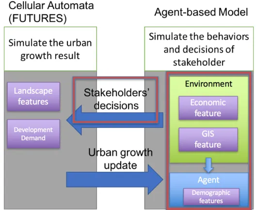
ABM simulates stakeholders’ behaviors and passes the final decisions of the stakeholders

to FUTURES. Then FUTURES synthesizes the decisions along with landscape features to

generate the urban growth simulation results and pass the growth update back to ABM. In

our work, we define the interface between FUTURES and ABM in each time step and the

logic flow of discrete time-stepped simulation.

In this section, we first introduce our study area and explain the data we collected. And

then we present the methodology of the framework implementation.

2.2.1 Study Area

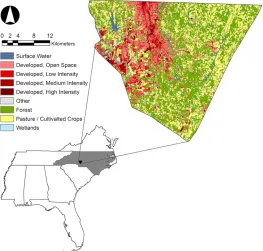
Cabarrus County is a region located in the north-east of Charlotte, North Carolina, USA,

as shown in Figure 2.1. Since the late 19th century, Cabarrus has been an area of cotton

cultivation and industrialization through cotton mills. Due to the economic development

of the Charlotte metropolitan area, Cabarrus County has significant urban growth in recent

decades. Despite the competitive advantage as being close to Charlotte, Cabarrus County

has a limited size of large-scale manufacturing and agriculture is still leading a dominant

role in its economy.

With the fact of mixed land use of agriculture and urban, Cabarrus County is an ideal

(20)

(21)

2.2.2 Data Description

To build an empirical model to simulate the urban growth in Cabarrus County, we collected

the demographic data, GIS data, and land market transaction data for the ABM module.

We use the census age and salary data of the residence to represent the social and

biologic status of the landowners. From the census data, we obtain the age and salary

distribution of Cabarrus County and interpolate the data for each landowner from the

distribution. Besides the census data, we also retrieved the land market transaction data of

Cabarrus County from 2004 to 2016. The transaction data contains the land transaction

history of the residential land use, farm land use, and commercial land use. We mainly

focus on the residential and farm land use in the data.

Besides the demographic and economic parameters, we use GIS measurement to

calcu-late the distance between each parcel to its closest green area and the highway. Distance to

park could reflect the living comfort degree, the closer the green area is, the more leisure the

residence could have, the fresher the air is. And the distance to the highway could present

the travel convenience levels. Since there’s no subway or many public transportation

op-tions in Cabarrus, the highway is the main transportation alternative. Therefore, we take

but not limited to the distance to green area (Dist2GA) and distance to highway (Dist2HW)

as the measurements of living comfort index.

We also collected the school rating scores of the primary, middle and high schools in

Cabarrus County. According to the school district division, we assign each household a

(22)

2.2.3 Framework Structure

We design an urban growth simulation framework that integrates an agent-based model to

simulate the stakeholder involvement. In addition to the cellular automata urban growth

simulation model, ABM plays an important role to simulate the behavior of stakeholders in

the urbanization problem.

Figure 2.2The communication between ABM and CA in each time step

As shown in the structure diagram in Figure 2.2, The framework is composed of CA and

ABM, we use FUTURES as our CA model. As the initialization requirement of FUTURES, we

initialize it with development demand and landscape features, such as slope, the distance

to city center, and etc. Once acquiring all the initializing data, FUTURES generates the

development potential DevPt of each landscape cell. Later FUTURES will use development

(23)

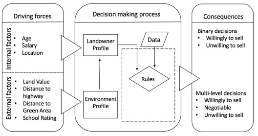
On the other side, ABM has two separate parts, they are environment and agent

sub-modules. Environment sub-module is responsible for collecting the data of the environment

where all the agents live in. In our design, we collect two kinds of data in the environment

sub-module, one is economic data such as land value, and the other one is GIS data such

as the distance to green area. And agent sub-module is the main reactor of ABM, it has the

ability to acquire the data from environment module and synthesizes its own demographic

data, also it could respond to the development request with landowner’s decision. All the

data we collected in our simulation can be considered as the drivers to the urbanization

process.

This design enhances the power of the framework to simulate a more empirical

simula-tion. The selection of the drivers reflects the understanding of the problem modeling, and

the implementation of each driver has a significant influence on the ultimate result of the

simulation. In our study, we have age and salary drivers to assign age and salary for each

landowner on the study area. And we also implement a land price estimator for each land

parcel in the study area. We apply GIS tools to calculate the distance between each parcel

to the nearest green area and highway.

Next, I will introduce more about the CA model in our framework, FUTURES.

2.3 FUTURES

FUTURES is a multilevel modeling framework for simulating changing regional urban-rural

divide based on observed land change patterns[Mee13]. It is a useful tool for researchers of urban systems to study the effect of changing landscape patterns with urbanization.

FUTURES considers a variety of environmental, infrastructural, socioeconomic and

(24)

Figure 2.3The FUTURES land change modeling framework[Mee13]

land growth patterns. These inputs are non-stationary drivers of land change influencing

the spatial structure of new growth regions and known to vary with time. Also, FUTURES

also considers simulated land conversion events in a feedback loop to predict new land

change patterns. To incorporate the different drivers of land change, the spatial structure

of land change events and their influence on further conversions, the FUTURES framework

couples three interacting components: a DEMAND sub-model that projects the estimated

demand for land in a region, a POTENTIAL sub-model that quantifies the site suitability of

land in a region and, a patch growing algorithm (PGA) that produces projections of regional

landscape patterns based on outputs from the DEMAND and POTENTIAL sub-models.

Figure 2.3 provides an overview of the FUTURES simulation framework and its

interact-ing components, namely, (i) DEMAND sub-model, (ii) POTENTIAL sub-model and, (iii)

Patch Growing algorithm (PGA)[Sha16].

The POTENTIAL sub-model implements a site suitability modeling technique that

(25)

infrastruc-tural, and socioeconomic changes over time in a region. The model considers a number

of predictor variables as input to a multilevel logistic regression model. Each predictor

variable accounts for a spatial or temporal aspect of land cover change and is used to define

a suitability score for a site in a region. Finally, the output from the POTENTIAL model is

normalized to produce a map of development probability values for all sites in a region.

The probability that an undeveloped cell becomes developed is defined as:

pi=

esi

1+esi

whereSi is the composite development potential for a celli. The development potentialSi

is defined as a function of environmental, infrastructural, and socioeconomic predictor

variables of site suitability as following:

Si=aj i+ n

X

h=1

βj i h∗xi j+βj i h∗p_i0

where, for theit_h_{undeveloped cell and varying across}_j _{groups (i.e., the level),}_a

j iis the

intercept,βj i is the regression coefficient,h is a predictor variable representing conditions

at the start of a chosen simulation year,n is the number of predictor variables,xi h is the

value ofh ati, andp0_{is the dynamic development pressure variable due to neighboring}

developed sites.

p_i0=

ni

X

k=1

S t a t ek

d_{i k}γ

whereS t a t ek is the current state (0/1) of thekthneighbor of celli,dis its distance from

thekth neighbor in its list of n neighbors andγis a coefficient that controls the influence

(26)

The DEMAND sub-model establishes the relationship between historical land

con-sumption and population growth under different development scenarios. This relationship

is established using an ordinary least squares regression technique. The regression model

considers two parameters in estimating future land use for urbanization: (i) population

growth and (ii) land consumption over time. The generated per capita demand projections

from the model drive the PGA in the FUTURES UGM.

The Patch Growing Algorithm implements the mechanism to simulate historically

observed urbanization patterns based on the above two sub-models. Patch growth is

de-fined as a 3-step process: (i) Monte Carlo based seed selection using the site development

probability, (ii) patch size selection from a library of patch sizes, a weighted distribution

of historically observed patch sizes, and (iii) patch growth through a neighbor discovery

process.

A neighborhood configuration specified at the start of the simulation defines the

neigh-bor discovery process. Further, a site suitability metric for newly discovered cells determines

the most suitable cells that go towards patch growth.

si=si0∗d

−α

wheres0_{is the underlying development potential of cell}_i_,_d _{is the distance of cell}_i

to seed andαis a patch compactness factor. The PGA continues the neighbor discovery

process by using the newly added neighbors as potential seed cells. Thus, the patch growing

algorithm continues till the value of patch size is met or else terminates when no more

(27)

2.4 Model Drivers

The initialization of the framework requires empirical input, this section introduces the

data preparation.

2.4.1 Demographic Data

For this study, we collected the Cabarrus County demographic data like age and income of

the household. According to the census data, we built distribution samplers for age and

salary. We use a normal distribution for each age group of the landowners. The census data

provides the number of people in each age group within each street block. We assume the

age of people falls into the normal distribution. Based on the age range and percentage

of each age group, we assign the landowner an age, and the age increased by one with the

simulation continues over years. We also simulate the death of a landowner. We assume

that after the age of 79 (US average Life expectancy), the landowner has a chance to survive,

otherwise, we replace a new landowner based on the age and salary distribution.

And we use a skewed distribution, chi-square distribution, to describe the salary

distri-bution over the landowners. As the feature of chi-square distridistri-bution, we use the median

value of the salary of each age group within each street block to obtain the degree freedom,

as the equation below.

m e d i a n=k(1₋ 2 9∗k)

3

Here,k is the degree freedom of the distribution, and according to the survey conducted

by Society for Human Resource Management, the average annual salary raise is about 3.1%

(28)

increase by a fixed rate every year.

The landowner could be replaced as a result of two reasons, one is the death of a

landowner, and the other is the land trade transaction. Either of the above occurs, a new

landowner will replace the old one. And a new landowner will occur when a new parcel is

developed.

2.4.2 Land Market

The land market is a crucial factor in our study, the prediction of the land price could affect

the demand and decision-making of the stakeholders. We built a land price estimator based

on the historical land price to estimate the land value over years for every parcel on the

map.

While some researches have focused on factors that may affect the land value of a region,

such as the human density and the distance to central business district; however, the data

we obtained is too scarce to implemented any existing complex land value prediction model

[McM96]. Therefore, we selected a straightforward method to estimate the land value based on the available data, and test the approach with the statistics data, which compare the

median value of the predicted land values with the actual land values distribution.

Obviously, not all the parcels were sold in the past years, limited to the scope of the

transaction data of the land trade, we need to interpolate the data for every parcel. We use

the K-nearest-neighbor algorithm to interpolate the land price for each year. For example, if

we want to know the land value of a parcel for a certain year, we locate the nearest neighbors

(geographical distance) which had been sold in the same year and calculate the average

value of its neighbors for the demand parcel. With this method, we calculated the land

(29)

Table 2.2Comparison of median value of land (per sqrt feet) value distribution before and after the interpolation

zipcode County 2013BM 2013AM 2014BM 2014AM 2015BM 2015AM 2016BM 2016AM

28027 Concord 86.41 82.32 90.67 89.77 95 92.23 100.67 96.7

28025 Concord 81.83 80.78 85.25 83.78 89.17 89.67 94.58 92.3

28081 Kannapolis 73.42 70.45 76.17 76.23 79.83 80.89 85 82.67

28083 Kannapolis 70.5 71.67 72.5 70.73 75.25 72.23 80.42 76.8

28075 Harrisburg 93.5 87.23 97.5 98.67 101.75 103.5 106.92 110.21

28107 Midland 99.33 95.45 102.3 98.98 106.17 104.56 112.08 105.4

28124 Mount Pleasant 93.41 93.56 97.75 94.4 100.17 100.4 104.33 102.7

BM is the median value of the land value distribution before interpolation, and AM

is the median value of the land value distribution after interpolation. From Table 2.2, we

can see the tendency of the land value for each zip-code in Cabarrus County. With the

development of economy and urbanization, the land value is increasing by years. And

we can also observe that the land value declines with the distance to Charlotte (in the

South-western of Cabarrus County).

Figure 2.4Cabarrus land value trend for zip code (2004-2006)

From Figure 2.4, we can clearly observe the tendency of the land value on Cabarrus

County, and the tendency of different zip-code area follow almost the same pattern. In

(30)

predict the land value based on the historical values. By interpolation and prediction of

the land value, we considered both spatial and temporal change of the land value, and the

historical land value could be well interpolated across the map.

2.4.3 GIS Data

GIS data is also widely used in the urbanization problem[CG98] [Bat07] [LY00] [Sud04], and the application of GIS in urban growth prediction propel the implementation of the models.

We use multi-layer data, GIS is applied as a data integrator. Although the data is already

existing, we created new maps to fit the grid resolutions and projections.

And the other purpose of using GIS is visualization. This is the weak component for

urban growth, GIS can just enhance the model. The role of GIS in for visualization is taking

the intermediate result and generate the visible map for the comparison of different maps.

The model we built requires the DIST2GA and DIST2HW as inputs to ABM, we projected

the shapefile of Cabarrus County transportation and Cabarrus County green land onto the

Cabarrus County land parcel, generating the raster file of the distance from each parcel to

its nearest highway and green area. With the same method, we also mapped each parcel

to corresponding schools (primary, middle and high schools), and calculate the average

school rating score for each parcel.

Up to this point, we prepared the initial data to train and test ABM, as listed as (i)

landowner age, (ii) landowner salary, (ii) land parcel distance to green area, (iii) land parcel

distance to highway, (iv) land parcel value, (v) land parcel school rating. With the above

data, we designed our discrete-time agent-based model to simulate the decision-making

(31)

2.5 Agent-based Model

To interact with urban growth model, the human involvement simulation should be

capa-ble of responding with the landowners’ decisions while retrieving sufficient information

for both the internal(landowner) and the external(environment) properties. With more

information considered, a simulating module could always generate better predictions. In

our design of the agent-based model, we fully considered the heterogeneity of the model,

each agent on the map is an autonomous individual[Zha16]. The system level behaviors emerge from the micro-level interactions of the agents. Therefore, it could depict the whole

simulation procedure with the details of different levels, specifically reasoning how and

when a decision is made by the landowners. Also, ABM aggregates all the information of its

constituent elements and measure the outcomes in the system level over time.

2.5.1 Agents Conceptualization

We conceptualize the model obeying ODD protocol[Gri10]. The ODD protocol is a standard format proposed to describe the individual and agent-based model.

The ABM is designed with two-layers, one is landowner layer, and the other is

environ-ment layer. As illustrated in Figure 2.5, available parcels (Not all the parcels are legitimate

for developing, such as roads) and all the landowners on the layers are conceptualized

as agents, which maintains the information passed by the model drivers. With the model

driver updating the values, the agents update its memory.

When the simulation starts, the landowner retrieves the land parcel information where

(32)

data. In our experiment, we tried various kinds of machine learning algorithms to test their

performance in this framework.

The key outcome of the model is the decision map, indicating if the landowner is willing

to sell some certain landscape cell to develop. And the FUTURES is seeking the objective

that the landowner is willing to sell this parcel based on the decision map generated by

ABM, and in return, the newly developed parcels trigger ABM generate new landowner

agents.

Figure 2.5Agent-based model conceptualization

The outcome of ABM synthesizes not only the landowners’ condition but also their

neighbors’ impact on them. Besides the agents internal updating, we also modeled the

influence of external agents of the experiments. In the experiment, we also tried different

mechanisms for different scenarios.

2.5.2 Agents Decision Rules

Traditionally, the decision of the landowner is simply yes or no, such implementation

(33)

make a decision based on the decision rules, and there’s also a development demand for

each year, this problem happens when the number of the willing landowner is less than the

demand. To solve this problem, we proposed a new decision hierarchy to replace the binary

yes/no. In our design, the decision is 3 categories as willingly, negotiable and unwillingly. When there are not enough â ˘AIJwillinglyâ ˘A˙I landowners, we will convert some negotiable

landowners into â ˘AIJwillinglyâ ˘A˙I ones by the process of bargaining. And the simulation

could continue with enough cells to develop.

We conclude the decision rules with some machine learning algorithms. For binary

de-cisions, we use the historical land transaction data to train our model. From the transaction

record, we can tell which cell is sold in which year, combining with other features which we

have initialized for each year, we can try to find the decision-making pattern. With logistic

regression algorithm, we can obtain the function with the parameter of age, salary, distance

to green area, distance to highway, land value and development potential.

When it comes to multi-level decisions, we cannot get such label from the historical

transaction record directly. We use the time interval between two transactions of the same

cell to determine the decision labels. When a piece of land is sold within a certain threshold,

we can infer that when a person with certain characteristics owns a piece of land, he is more

likely to sell it. The threshold we use is the average moving time of US residence, it is 5 years.

So we define that when the interval is less than 4 years, the stakeholder is more willing to

move, and longer than 6 years is unwilling to move. Any other time between 4 and 6 years,

which contains 5 is negotiable to move. We test different classification algorithms to train

(34)

2.5.3 Agents Neighbor Influence

We consider the neighborhood influence among agents. And For a different decision setting,

we have different influence calculation methods. For binary decision, since we are using

logistic regression, we find a way to aggregate itself value and its neighbors. For multi-level

decisions, we define a cross-reference table for neighborhood influence as shown in Table

2.3. In the neighborhood, we apply majority voting, selecting the most popular decision

and consider both the local and neighbor decision, according to the table, we have the final

decision.

Table 2.3Neighborhood Influence for multi-label approach

Willingly Negotiable Unwillingly Willingly Willingly Willingly Negotiable Negotiable Willingly Negotiable Unwillingly Unwillingly Negotiable Unwillingly Unwillingly

2.5.4 Agent’s Bargain Process

We implement multi-level decision because of insufficient cells to develop in the

urban-ization process. And in an empirical study, developers would like to negotiate with the

landowners or providing them a higher bid[PF08]. When adopting the multi-level deci-sion, we need to consider converting negotiable landowners into willingly ones, and in the

meantime, the land value should increase by a certain percentage. The increasing rate is

(35)

2.6 Experiments

We split the experiment into four parts, the first part is to train the model to generate the

decision-making rules for the landowners, to test under what circumstances that they

would sell their land. The rest of the experiments are all conducted in the form as the

comparison of 3 platforms as the plain FUTURES, the FUTURES with binary decision ABM

and the FUTURES with the multi-level decision. And the second experimental part is to

simulate without neighborhood influence, and the third experimental part is to simulate

with neighborhood influence. The fourth experimental part is to simulate with

neighbor-hood influence and the bargaining process. Additionally, before the fourth experiment, we

need to determine the land value increase rate.

All the experiments were initialized with different scenarios of different landowner age

and salary assignment. For each scenario, we repeated the experiment 10 times, and we

summarize all the result to get an average value for validation. The simulation year is from

2014 to 2016.

2.6.1 Validate Metrics

We used two validation metrics in the result analysis of our experiment, they are allocation

agreement and willingness agreement. Allocation agreement indicates the precision of the

urban growth simulation prediction, representing the ratio of correctly predicted developed

cell status.

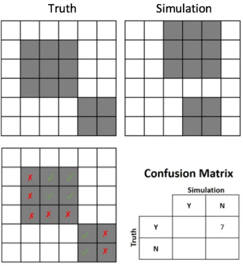
As illustrated in Figure 2.6, the allocation agreement is the ratio of the overlapping

(36)

Figure 2.6Allocation agreement illustration

Al l o c a t i o n Ag r e e m e n t = N u m(T P)

N u m(T P) +N u m(F P) +N u m(T N) +N u m(F N)

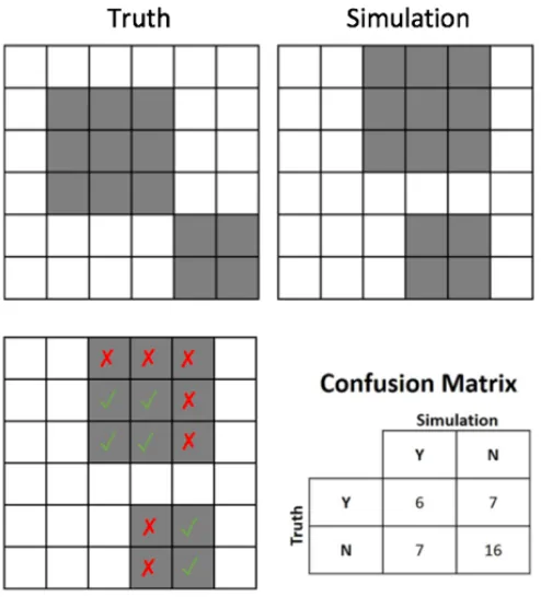
And the other metric is willingness agreement. Willingness agreement is the

measure-ment for the performance of the agent-based model, representing the ratio of correctly

pre-dicted decisions. Since we don’t know the actual decisions of the landowners, we could only

imply that via the actual development map. We compare the predicted decision-making

result with the actual development map. As shown in Figure 2.7, we can only retrieve the

false negative in the confusion matrix, and we are not sure about others. So, we defined the

(37)

Figure 2.7Willingness agreement illustration

W i l l i n g n e s s Ag r e e m e n t = N u m(F N)

N u m(T P) +N u m(F P) +N u m(T N) +N u m(F N)

2.6.2 Train the Model

We obtained the historical transaction data for each parcel, we use this dataset to train and

test the performance of different machine learning algorithms. Along with this dataset, we

assign an age and salary to the landowners based on the model drivers, the DIST2GA and

DIST2HW to each, and the sold price (per sqrt feet) from the record, and also generate the

(38)

item in the transaction record, we have the landowner age, landowner salary, DIST2GA,

DIST2HW, land value, development potential and the sold status, which is the decision of

the landowners. We regard the other parcels which are not listed in the record as unsold.

For this raw and extended dataset, we have 59136 sold records and 1350740 unsold

records, and we use the data record from 2004 to 2013 as training data, and the rest as

testing data.

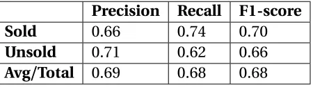
We use logistic regression[KZ01] [BH03]to generate binary output as the decision of the landowners. Table 2.4 is the result of the test:

Table 2.4Logistic Regression result

Precision Recall F1-score

Sold 0.66 0.74 0.70

Unsold 0.71 0.62 0.66

Avg/Total 0.69 0.68 0.68

We calculated the intervals of transactions of each parcel, retrieving the multi-label

decision of the landowners.

Table 2.5, Table 2.6, Table 2.7, Table 2.8 are the results of different algorithms:

Table 2.5CART result

Willingly 0.74 0.73 0.74

Negotiable 0.70 0.70 0.70

(39)

Table 2.6SVM result

Willingly 0.54 1.00 0.70

Negotiable 0.99 0.23 0.37

Unwillingly 1.00 0.27 0.42 Avg/Total 0.60 0.60 0.53

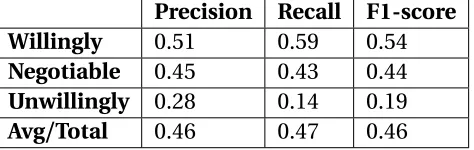
Table 2.7Bayesian Network result

Willingly 0.51 0.59 0.54

Negotiable 0.45 0.43 0.44

2.6.3 Simulation

We chose random forest as the multi-label algorithm to compare with binary output result

since it has the moderate but steady performance among the competitors.

we took 2013 as a starting year and test the development status of 2014, 2015 and

2016. We did three simulations with different conditions, we tested the framework with the

plain frameworks, FUTURES model alone, FUTURES model with binary decision ABM and

FUTURE model with multi-level decision ABM. Firstly, we assume that the landowners are

not affected by its neighbors (adjacent parcels) and no bargaining process involves. And

(40)

Table 2.8Random Forest result

Willingly 0.74 0.76 0.75

Negotiable 0.70 0.71 0.70

last, we added the bargaining process when dealing with multi-level decision ABM model.

Before the simulation, we need to determine the optimal land value increase rate of the

bargaining process. As shown in Figure 2.8, we increase the rate from 5% to 15% by the

interval of 0.5%. And the result shows that with the rate of 8%, it gives the best simulation

result.

Figure 2.8Prediction accuracy with land value increase rate change

(41)

Table 2.9Simulation Result without Neighborhood Influence

Year Framework Demand Successfully Developed Allocation Agreement Willingness Agreement 2014 Plain Futures

9773 9773 17%

-2015 9773 9773 15%

-2016 9773 9773 14%

-2014

Binary Decision

9773 9773 18% 35%

2015 9773 8750 17% 46%

2016 9773 - -

-2014

Multilevel Decision

9773 9773 24% 44%

2015 9773 6164 20% 60%

2016 9773 - -

-Table 2.10Simulation Result with Neighborhood Influence

9773 9773 16%

-2015 9773 9773 16%

-2016 9773 9773 14%

-2014

Binary Decision

9773 9773 20% 40%

2015 9773 7896 19% 45%

2016 9773 - -

-2014

Multilevel Decision

9773 9773 29% 60%

2015 9773 6164 22% 62%

(42)

-Table 2.11Simulation Result with Neighborhood Influence and Bargain

9773 9773 17%

-2015 9773 9773 16%

-2016 9773 9773 15%

-2014

Binary Decision

9773 9773 22% 48%

2015 9773 7654 19% 45%

2016 9773 - -

-2014

Multilevel Decision

9773 9773 32% 60%

2015 9773 9773 24% 62%

2016 9773 9773 26% 68%

2.7 Results and Analysis

From the results of the experiment, on average, the binary and multi-level framework

out-perform the plain model of FUTURES alone for both the overlapping rate and disagreement

rate. And in the comparison with binary and multi-level decision framework, multi-level

decision framework performs better. In the first and second experiment, multi-level

ap-proach failed in development enough parcels, so the land growth model quit in developing.

The reason for that is there are not sufficient landowners agree to sell their land, and the

developers do not negotiate with these landowners. The overlapping rate of the multi-level

approach is lower than the third experiment, one of the reasons is that the fewer number

of the cells were developed. However, the disagreement rate is lower than the other two

approaches in the first experiment.

When adding neighborhood influence, we noticed that the performance of all has been

(43)

That indicates that when the interaction between landowners occurs, the landowner learns

more of the environment through his/her neighbors, which helps the landowner make the correct and wise decision.

In Table 2.10, Multi-level approach met the demand of development with moderate

per-formance. When the bargaining process involved, we can see that the allocation agreement

rate is raised, which verifies our assumption that neighborhood influence and bargain

process could improve the landowner agents’ ability to make more intelligent decisions.

And the land value increase rate indicates the commercial pattern in land trade. When the

value of the land is low, fewer landowners would like to sell their land; and when the land

value is too high, the allocation agreement rate drops because of fewer developers would

like to buy and develop a new site.

Besides the spatial error estimation, temporal error estimation is also important. Error

propagation exists in the simulation. We did another experiment to test the impact of error

propagation that small initial error in geo-simulation will lead to larger errors in the end.

We manually inserted incorrect data into our initial landscape file. We randomly selected

10%, 15%, and 20% cells on the map, transposing their development status. With such

preparation, we intentionally aggrandized the initial error in order to observe the impact of

error propagation.

(44)

CHAPTER

3 BUILD ABM ON APACHE SPARK

3.1 Problem Statement

Urbanization is a process that accumulates for a long time. Therefore, a significant change of

the land use could take place after years. In the prediction of the urban growth, researchers

usually measure the land use status of the past years and simulate the following land use

status of the next decades.

Many factors would affect the urban growth and development, including the properties

of the landscape and landowners. For a better illustration of the algorithm and model, we

(45)

Landscape cell: We grid segment the landscape, and each grid of the landscape is called

a cell.

In many spatial problems, satellite images are used for further analysis. We can

re-gard each pixel of the image as a cell. And in some actual landscape maps, we use such

representation to convert continuous data into discrete data.

Landscape parcel: A group of adjacent cells which belong to the same landowner is call

a parcel.

A landowner may have more than one parcel on the landscape, and all of the parcels

from the same landowner may sparsely locate.

We also define one spatial relationship of the landscape parcels.

Parcel neighborhood: A group of parcels which are adjacent to a parcel, is called this

parcel’s neighborhoods.

For instance, we assume there is one piece of the landscape taken into consideration,

as shown in Figure 3.1. Each color area indicates a landscape parcel, and each parcel is

composed of multiple cells, as represented by dotted squares. For better illustration, we

mark each parcel a name alphabetically. As defined above, only the adjacent parcels are

considered as the neighborhood of a particular parcel. In this example, parcel A’s neighbors

are C, D, E, F, G, H.

Hence, we have an overview of the landscape units and the relationships between them,

and we would specify the problem we are facing. Human involvement is inevitably in

urbanization, and people have the ownership of the land and the willingness to trade. Also,

one person’s decision could be affected by others, like peers or neighborhood. We need a

module simulating and monitoring human involvement and conduct further qualitative

and quantitative analysis.

(46)

Figure 3.1Example of landscape cell, landscape parcel and parcel neighborhood

information as input, including the landscape cells’ position, landscape parcel composition,

landscape parcel ownership, the profiles of landowners and other landscape information

whichever used in the decision-making algorithms. With the information of landscape and

landowners, this module could calculate the probability of how likely the landowner is

willing to sell a certain parcel and make the ultimate decision of the landowner. Since this

module is working with the urban growth simulation model, it could respond to the urban

growth model when it’s requested to provide the final decision if any parcel is going to be

sold or not.

Since the urban growth simulation is usually done for decades in the future, researchers

usually simulate not for a single year, but a series of continuous years. In our study, we

(47)

multiple-year simulation as working with both an urban growth simulator (UGS)and a human

involvement simulator (HIS). UGS waits for the feedback from HIS, the response time of

HIS is the gap of the overall performance; we aim to reduce the response time of HIS to

improve the performance of the simulation.

Figure 3.2Communication between Urban Growth Simulator and Human Involvement Simula-tor for Rounds

Building a stable and scalable human involvement simulating module can assist the

urban growth model to make a more accurate prediction, and help people analyze how

human affect the urbanization procedure.

3.2 Methodology

To interact with urban growth model, the human involvement simulating module should be

capable of responding with the landowners’ decisions while retrieving sufficient

(48)

Figure 3.3Human involvement module communicates with urban growth model

module could always generate better predictions. In our study, we pass the landowners’

profile and landscape geographic information as an initial input to the human

involve-ment simulating module; some decision-making algorithms could convert the data into

landowner’s decisions.

3.2.1 Formulas

We consider landowner’s the probability of the landowners’ willingness to trade their land

is based on the parcel, which means we assume that all the land trades are in the unit of a

parcel. However, all the landscape information we gathered is based on landscape cells,

we need algorithms to transfer the landscape information from cell level to parcel level.

Before introducing the algorithms, we need to define some critical parameters we used in

the algorithms.

Development potential: Development potential is a value indicating how likely a cell

would be developed into an urban area without human involvement.

While urban growth model is working in a standalone mode, development potential is

(49)

with the innate and acquired conditions of the landscape cells, as well as the adjacent cells’

information. Development potential synthetically considers the interior and the exterior of

the landscape conditions.

Willingness to sell: Willingness to sell (WTS) is a value indicating how willing a landowner

would be to sell the landscape cell or parcel.

When human involvements occur, the intention of the landowners becomes crucial. In

the trade of one piece of land, landowners always synthesize multiple factors and make the

final decision if the land could be sold or not. And during the decision-making procedure, a

landowner could also be influenced by other landowners. Due to the different personalities

of the landowner, their behavior can be varied in pondering the decision. Overall possible

influencing factors, we use WTS to represent the possibility a landowner could sell a certain

cell or parcel.

As shown in Figure 3.4, a cell’s WTS should be calculated based on the landowner

information and its development potential, the algorithm we use to calculate cell’s WTS is

illustrated as below.

LetW T Sc e l l to be the willingness to sell value of a landscape cell, and potential to be

the development potential value of this landscape cell. If a landowner owns this landscape

cell, we assume that

W T Sc e l l =i n t e r s e c t i o n+α∗a g e+β∗i n c o m e+γ∗p o t e n t i a l

wherei n t e r s e c t i o nis a value that varies among different types of landowners,a g e

is the age of the landowner, andi n c o m e is the annual income of a landowner.α,β,γare

the coefficients of the parameters. In our study, we useαas 0.0032,β as 0.00000486, andγ

(50)

Figure 3.4Working flow of urban growth model and human involvement simulating module for one-time step

Since our study is based on landscape parcels, we should obtain the intention of the

landowner about the whole parcel. We also use the value willingness to sell to represent the

intention of the landowner.

letW T Sp a r c e l to be the willingness to sell value of a landscape parcel andW T Sc e l l to

be the willingness to sell value of a landscape cell. We have

W T Sp a r c e l =

P

c e l l∈p a r c e lW T Sc e l l

P

(51)

We use the averageW T Sc e l l in a parcel to signify the willingness to sell a parcel.

Not only the internal factor influencing the decision of the landowners, but they could

also be affected by their peers, such as their neighborhood, workmates or some financial

agents. We usep e e r i n f l u e n c e to measure the outside influence on the landowners. In

our study, we only consider the situation when the landowners are influenced by their

neighborhood, specifically the other landowners who own the adjacent parcels.

LetP to be the peer influence value of one certain parcel, and we can calculateP with

its adjacent parcels’W T S.

P =

P

p a r c e l∈n e i g h b o r h o o dW T Sp a r c e l

P

p a r c e l∈n e i g h b o r h o o d1

The averageW T S value of the neighborhood is regarded as the peer influence on a

certain parcel, which can be interpreted as the more willingly the neighborhood to sell their

land, the more likely a landowner would be to sell the land.

We have obtained theW T Sof the landscape parcel and the peer influence to it, however,

they have different dominants, we need to normalize the values before conducting more

operations on them. The normalization method we use is as below.

LetN o r m a l i z e d be the normalized variable, and x to be the original value.

N o r m a l i z e d= e

x

1+ex

Hence, we have the normalized parcel W T S and peer influence; we plan to test how

the urbanization differentials when given different proportions of parcelW T S and peer

influence.

LetDVp a r c e l to be the determinative value for the landowner,W T Sp a r c e l to be

(52)

peer influence.

DV =α∗W T Sp a r c e l+β∗P

αandβ are the coefficients we would give to the function when testing, indicating

the proportion of the parcel’sW T S and peer influence. For keeping the consistency of

normalization, we simply should have the equationα+β=1.

With the normalized determinative value of the decision, we can set an arbitrary

thresh-old for the landowners to make the ultimate decision.

LetR AN D be the random threshold we set for the landowner to make a decision,DV

to be the determinative value of the decision andD T S to be the decision to sell.

D T S=1,w h e n DV ≥R AN D

D T S=0,o t h e r w i s e

Human involvement simulating module passes the decision of the landowner to the

urban growth model, assisting urban growth model to accomplish the urbanization

simu-lation.

3.2.2 Agent-based Model

Agent-based modeling (ABM) is widely applied in the domain of dynamic simulation of

the geographical system in the last decade. A definition is provided by Axtell: "An ABM

consists of individual agents with states and rules of behavior. Running such a model is

simply creating a population of such agents and letting agents interact, and monitoring

(53)

through the simulation of human involvement during the urbanization.

Agent-based modeling is a technique for modeling dynamic systems from the bottom

up. Individual elements of the system are represented computationally as agents. The

system level behaviors emerge from the micro-level interactions of the agents. Therefore, it

could depict the whole simulation procedure with the details of different levels, specifically

reasoning how and when a decision is made by the landowners. Also, ABM aggregates all

the information of its constituent elements and measure the outcomes in the system level

over time.

There are several features of the agents in most of the agent-based models, which are

briefly illustrated below[CH12]:

• Autonomy: all of the agents are autonomous entities, their functionalities are not

affected by the system or other agents. The agents should have the ability to process

the data internally and communicate with the environment and other agents through

messages.

• Heterogeneity: the agents can be in different shapes of entities. Various agents

main-tain different sets of attributes and functions. Also, a group of the same kind agent is

allowed as long as they have a similar set of attributes and functions.

• Active: all the agents contribute to the simulation outcomes.

All the agents together amalgamate the agent-based model, and different types of agents

have different jobs in the simulation. The human involvement simulating module could be

shaped into an agent-based model. And in this way, we can better interpret the relationships

among different types of agents and observe the state change of agents.

three principal components to be documented about a model: Overview, Design

(54)

3.3 Model Overview

3.3.1 Model Design Concepts

The key outcome of the model is the decision raster file, indicating if the landowner is

willing to develop some certain landscape cell. The outcome synthesizes not only the

landowners’ condition but also their neighbors’ impact on them. All of the landscape

cells, parcel and landowner have adaptive behavior, as landscape updates development

potential and landowner updates age after each time step, and landscape parcel updates

its willingness to sell value once it senses the landscape cell holds a new willingness to sell

value. And the landscape parcel is seeking the objective that the landowner is willing to

sell this parcel. Stochasticity is used to determine the threshold to make the final decision.

Also, a set of collective jobs is presented in the model, as the landscape cells within the

same landscape parcel working as a group, their average value of willingness to sell is one

of the landscape parcels, and they share the same DTS value; and the landscape parcel

neighbors work in the shape of a group as well. Moreover, the agents interact with each

other via messages.

3.3.2 Model Details

• Initialization

Since all the raw landscape data is in the format of raster and the landowner profile is

in the format of tables, we need to reassign all the data to corresponding agents.

• Input data

(55)

sim-ulation model, and the input data for each time step is passed in by urban growth

simulating model as the updated development potential value of every landscape

cell.

• Output data

After each time step, the human involvement simulating module generates a raster

of the landowner’s decision on every landscape cell. The raster file indicates if the

landscape cell in the corresponding position of the landscape earns the permission

from its landowner to be traded for development into the urban area.

• Purpose

The purpose of this model is to simulate the human involvement in urban growth

procedure, especially the decision making of landowners in the land trade.

• Entities, state variables, and scales

We briefly categorize the agents into three types: landowners, landscape cells and

landscape parcels. And the state variables of each type of agents are listed below

correspondingly:

– Landowner

Landowner ID: the unique identification of a landowner.

Landowner Type: There are four types of landowners, we assume they would

hold different attitudes when the land trade is happening. The main

differ-ence among the four types of landowner in computation is embodied in

landscape cell’s willingness to sell (WTS) value. The more conservative the

(56)

Landowner Age: the age of the landowner.

Landowner Income: the annual income of the landowner.

– Landscape Cell

Landscape Cell ID: the unique identification of a landscape cell.

Landscape Parcel ID: the id of the landscape parcel that this landscape cell

locates in.

Landowner ID: the id of the landowner who owns this landscape cell.

Development Potential: the development potential value of this cell, this

variable is estimated by urban growth model and passed in.

WTS: value of willingness to sell by the landowner on this landscape cell.

DTS: value of the decision to sell by the landowner on this landscape cell.

– Landscape Parcel

Landscape Parcel ID: the unique identification of a landscape parcel.

Landowner ID: the id of the landowner who owns this landscape parcel.

Landscape Cell List: the ID list of the landscape cells which locates in this

landscape parcel.

Neighborhood Parcel List: the ID list of the landscape parcels which locates

adjacent to this landscape parcel.

Peer Influence: the value of the peer influence to this landscape parcel.

WTS: value of willingness to sell by the landowner on this landscape parcel.

DTS: value of decision to sell by the landowner on this landscape parcel.

(57)

The communication among agents to agents or agents to the environment occurs

via messages. Before introducing the functions of different agents, we define some

messages in the communication.

– Message of Landowner Information

sender: landowner

receiver: landscape cells under the landowner’s property

content: the landowner’s profile, including the landowner’s ID, typology,

age and income

– Message of Landscape Cell’s WTS

sender: landscape cell

receiver: the landscape parcel which the sender in

content: the landscape cell’s ID and WTS

– Message of Landscape Parcel WTS

sender: landscape parcel

receiver: the landscape parcels which locates adjacent to the sender

content: the landscape parcel ID and WTS

– Message of Landscape Parcel DTS

sender: landscape parcel

receiver: the landscape cells which locates into the sender

The Smart Agent-based Model in Urban Growth Problems.

ABSTRACT

DEDICATION

BIOGRAPHY

ACKNOWLEDGEMENTS

TABLE OF CONTENTS

LIST OF TABLES

LIST OF FIGURES

CHAPTER

1

INTRODUCTION

CHAPTER

2

SAMRT AGENTS IN URBAN GROWTH

SIMULATION

2.1

Related Work

2.2

Methods

2.2.1

Study Area

2.2.2

Data Description

2.2.3

Framework Structure

2.3

FUTURES

2.4

Model Drivers

2.4.1

Demographic Data

2.4.2

Land Market

2.4.3

GIS Data

2.5

Agent-based Model

2.5.1

Agents Conceptualization

2.5.2

Agents Decision Rules

2.5.3

Agents Neighbor Influence

2.5.4

Agent’s Bargain Process

2.6

Experiments

2.6.1

Validate Metrics

2.6.2

Train the Model

2.6.3

Simulation

2.7

Results and Analysis

CHAPTER

3

BUILD ABM ON APACHE SPARK

3.1

Problem Statement

3.2

Methodology

3.2.1

Formulas

3.2.2

Agent-based Model

3.3

Model Overview

3.3.1

Model Design Concepts

3.3.2

Model Details