PERFORMANCE OF FREQUENCY ANALYSIS FOR ESTIMATING DESIGN RAINFALL (CASE STUDY ON THE UPSTREAM LESTI SUB-WATERSHED)

(1)

Performance of Frequency Analysis for Estimating Design Rainfall (Case Study on

the Upstream Lesti Sub-watershed)

Ery Suhartanto

1

, Lily Montarcih Limantara

1

, Tris Raditian

2

, M. Firman

2

and Musdiyanto Mukhti

2

1_{Lecturer in the Department of Water Resources, Faculty of Engineering, University of Brawijaya, Jl. MT Haryono No. 167 Malang 65145, East Java of}

Indonesia.

2

Doctoral Program in the Department of Water Resources, Faculty of Engineering, University of Brawijaya, Jl. MT Haryono No. 167 Malang 65145, East Java of Indonesia.

Article Received: 22 September 2017 Article Accepted: 25 December2017 Article Published: 12 January 2018

1. INTRODUCTION

Over the past several decades, rainfall over Indonesia has been decreasing significantly, which causes a decrease in

dam inflow as a result. This has attracted significant interest and attention, particularly in terms of possible causes

and policy options in response to the decrease [1]. While not conclusive in terms of possible drivers of the rainfall

decrease, an important finding is that since the middle of the twentieth century, the rainfall decreases at the specific

stations and the decrease occurred through reductions in the number and intensity of the extreme events [2][3].

Rainfall is a phenomenon characterized by the high variability both in the space and time [4][5], which makes its

measurement difficult. Even though rain gauges provide accurate rainfall measurements, these are only

representative for a limited spatial extent. Over the vast majority of the globe, rain gauge networks are too sparse

(or completely missing) to capture the variability of the precipitation systems in space and time [6]. The heavy

rainfall events can trigger natural disasters, such as flooding and landslides. An important concern is whether the

future climate change will alter the intensity and frequency of the extreme rainfall and how it will affect the

characteristics of the extreme rainfall [7]. The previous studies have indicated that the frequency and intensity of

extreme rainfall on a daily basis exhibits a positive trend but that there are the large regional differences in the level

of the increase or decrease [8][9]. However, such the increases are attributed especially to the uppermost percentile

of the global rainfall distribution [10]. The extreme rainfall is associated with a wide variety of the weather systems,

such as the mesoscale convective systems [11], the orographic precipitation in association with the low-level jets

[12][13], the tropical cyclones [14].

Lesti sub-watershed is as part of the Brantas watershed which has the estuary in the Sengguruh reservoir. The

higher erosion level in the Lesti sub-watershed is caused by the topographical form which part of them is A B S T R A C T

The Lesti sub-watershed is as part of the Brantas watershed which the catchment area is 61,491.02 ha. Basically, the source of overall water that is flowing in the river and storage as the surface or sub-surface is the rainfall. Therefore, there is a relation between the rainfall and the river discharge in a watershed. The rainfall intensity in the Lesti sub-watershed is high enough and it causes the flooding, so it is needed the design of flood control. The type of rainfall that is needed for designing the water utilization and flood control is area rainfall. This study intends to estimate the design rainfall with some return periods. The methodology consists of the frequency analysis due to the distributions of Normal, Log Normal, Log Pearson Type III, and Gumbel. The result is hoped to be used for supporting the design of water utilization and flood control.

(2)

enough problem towards the area damage, erosion, landslide, river discharge fluctuation, and the sedimentation is

high enough. Therefore, the potency of water in it cannot be optimally used and it the dry season, there will be

happened the water deficit, however due to the bad system of water sources in the watershed, the rainfall intensity is

high enough so that it causes the flooding.

This study intends to analyze the design rainfall in the Lesti sub-watershed. To reach the objective, it has to be

analyzed the area rainfall by using the methods of arithmetic. Then, it can be carried out the analysis of design

rainfall by using the frequency analysis such as the distributions of Normal, Log Normal, Log Pearson Type III, and

Gumbel. The suitable distribution is depended on the testing of goodness of fit by using the Smirnov-Kolmogorof

test and chi-square.

2. MATERIALS AND METHODS

2.1 Study location

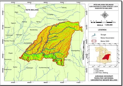
The upstream Lesti sub-watershed is located on the south longest of 8°02’50’’- 8°12’10’’ and the east longest of

112° 42’58’’- 112°56’21’’ and it is in the Malang regency. This area has the heterogenic characteristic on the basic

physical condition. Delineation of the research area uses the ecological boundary such as the upstream Lesti

sub-watershed that is determined by the Brantas watershed institution. Map of study location is presented as in the

Figure 1.

(3)

2.2 Data collecting

The secondary data are needed in this study. The secondary data is as the data which is obtained from several

sources and can be accounted the accuracy. The secondary data that is collected for this study is as follow:

1. The daily rainfall data from the Poncokusumo station (2007-2016).

2. The daily rainfall data from the Dampit station (2007-2016).

2.3 The steps of study

The steps of study are systematically set for making easy to handle the solution. The steps of analysis are as follow:

2.3.1 Analysis of area rainfall

Analysis of area rainfall is carried out by using the arithmetic mean. This method is used for the area less than

50,000 ha. The result of this method is not far different with the other method if there are many rainfall stations and

the stations are equally distributed in the watershed. The advantage is this method is more objective than the Isohiet

method [15]. The formula of arithmetic mean is as follow:

P=1/n(P1+P2+…+Pn) (1)

Where:

P = area rainfall (mm)

P1,P2,…, Pn = rainfall in every observed point (rainfall station) (mm)

n = number of observed point (station)

2.3.2 Analysis of frequency distribution

There are 4 frequency distribution which will be used for analysis design rainfall in the Lesti sub-waterhed such as

the methods of Normal, Log Normal, Log Pearson Type III, and Gumbel

2.3.2.1 Normal distribution

The Normal distribution or Normal curve is also mentioned as the Gauss distribution. The formula for calculating

the estimation value with the return period of T (Xt) is as follow:

(1)

Where

XT : estimation of value which is hoped to be happened by the return period of T

X : mean

S : deviation standard

KT : factor of frequency which is as the function of probability or return period and as the type of

(4)

2.3.2.2 Log Normal distribution

The formula of Log Normal distribution is the same as the Normal distribution, but the data have to be transformed

into log.

(2)

Where

XT : estimation of value which is hoped to be happened by the return period of T (in the log)

X : mean (in the log)

S : deviation standard (in the log)

mathematical modeling of the probability distribution that is used for the probability analysis

2.3.2.3. Log Pearson Type III distribution

To use the Log Pearson Type III, the data have to be transformed into the Log form. The formula of Log Pearson

Type III with the return period of T (Xt) is as follow:

Log XT = Log X + K.s (3)

Where:

Log XT : estimation of value (in the Log from) which is hoped to be happened by the return period of T

X : mean (in the Log form)

S : deviation standard (in the log form)

mathematical modeling of the probability distribution that is used for the probability analysis

2.3.2.4. Gumbel distribution

The formula of the Gumbel distribution that is used for estimating the value which is hoped to be happened with the

return period of T(Xt) is as follow:

(4)

Where,

Xt = design rainfall in the return period of T year (mm)

X = mean rainfall of the observed result

Yt = reduced variate that is as the Gumbel parameter for the return period of T year

Yn = reduced mean that is as the function of the data number= f(n)

Sn = reduced deviation standard that is as the function of the data number = f(n)

(5)

2.3.2.5. Smirnov–Kolmogorov Test

This test intends to evaluate the horizontal deviation such as the maximum deviation between theoretical and

empirical distribution. The formula is as follow:

 maks = [ Sn - Px] (6)

Where:

maks = the deviation between theoretical and empirical distribution

Sn = theoretical probability

Px = empirical probability

If  maks < cr, the data are suitable with the distribution. The steps of Smirnov-Kolmogorof test are as follow:

a. To rank the data (from small to big or big to small) and to calculate each probability due to the ranking,

it is mentioned as the empirical probability.

b. To determine each of the theoretical probability.

c. To analyze the deviation between the theoretical and empirical probability

d.  maks is compared with the Δ critic form Smirnov-Kolmogorof table (Dcr).

2.3.2.6. Chi- Square test

Chi-square test intends to evaluate the difference between the sample data and the probability distribution. The

formula of chi-square test is as follow:

(7)

Where:

X2 = calculated chi-square

Ei = frequency that is hoped regarding to the class division

Oi= frequency on the same class

N =number of class. The formula of Ei is as follow:

. (8)

Where:

n = number of data

(6)

3. RESULTS AND DISCUSSION

Analysis of area rainfall in the Lesti sub-watershed is due to the method of arithmetic mean. Then, it is carried out

to analyze the design rainfall with some return periods by using the distribution methods of Normal, Log Normal,

Log Pearson Type III, and Gumbel.

3.1. Analysis of area rainfall

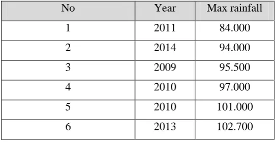
There are 2 rainfall stations in the study location. In hydrological analysis, the rainfall data are come from the two

station which is influenced to the Lesti sub-watershed. The rainfall data is from 2007 until 2016. Table 1 presents

the mean rainfall in the Lesti sub-watershed.

Table 1. Mean rainfall in the Lesti sub-watershed

No. year Poncokusumo station Dampit station Mean

1 2007 151.00 137.00 144.00

2 2008 150.00 117.00 133.50

3 2009 85.00 106.00 95.50

4 2010 94.00 108.00 101.00

5 2011 79.00 89.00 84.00

6 2012 110.00 109.00 109.50

7 2013 115.00 79.00 97.00

8 2014 81.00 107.00 94.00

9 2015 89.00 117.00 103.00

10 2016 50.00 155.40 102.70

Source: own study

3.2. Analysis for selecting the suitable frequency distribution

Table 2 present the analysis for selecting the suitable distribution for Lesti sub-watershed.

Table 2. Analysis for selecting the suitable frequency distribution in the Lesti sub-watershed

No Year Max rainfall

1 2011 84.000

2 2014 94.000

3 2009 95.500

4 2010 97.000

5 2010 101.000

(7)

8 2011 109.500

9 2008 133.500

10 2007 144.000

Mean (X) 106.42

Deviation standard (S) 18.48

Skewness (Cs) 1.26

Kurtosis (Ck) 0.96

Coefficient of variation

(Cv) 0.17

Source: own study

3.3. Analysis of frequency distribution

To select the method of frequency distribution analysis for the rainfall in the Lesti sub-watershed, there is used the

methods of Normal, Log Normal, Log Pearson Type III, and Gumbel.

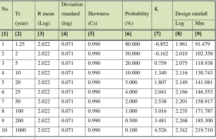
3.3.1. Metode Normal

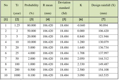
Table 3 presents the analysis and the result of design rainfall by using the Normal method. However, Table 4 and 5

present the testing of goodness of fit each for Smirnov-Kolmogorof Test and chi-square test.

Table 3. Design rainfall by using Normal method

No Tr Probability R mean Deviation

standard K Design rainfall (X)

(year) (%) (mm) (Sd) (mm)

[1] [2] [3] [4] [5] [6] [7]

1 1.25 80.000 106.420 18.484 -0.840 90.894

2 2 50.000 106.420 18.484 0.000 106.420

3 5 20.000 106.420 18.484 0.840 121.946

4 10 10.000 106.420 18.484 1.280 130.079

5 20 5.000 106.420 18.484 1.640 136.734

6 25 4.000 106.420 18.484 1.708 137.997

7 50 2.000 106.420 18.484 2.050 144.312

8 100 1.000 106.420 18.484 2.330 149.487

9 200 0.500 106.420 18.484 2.580 154.108

10 1000 0.100 106.420 18.484 3.090 163.535

(8)

Table 4. Smirnov-Kolmogorof for Normal method

a D critic D max Note

0.2 0.320 0.209 Accepted

0.1 0.370 0.209 Accepted

0.05 0.410 0.209 Accepted

0.01 0.490 0.209 Accepted

Source: own study

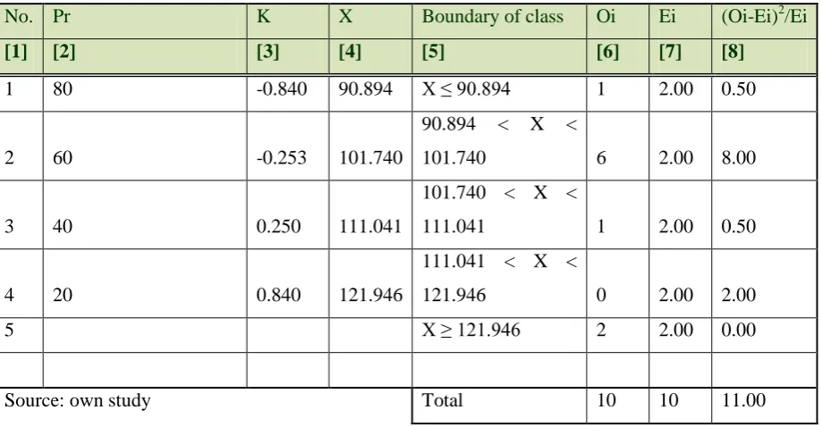
Table 5. Chi-square test for Normal method

No. Pr K X Boundary of class Oi Ei (Oi-Ei)2/Ei

[1] [2] [3] [4] [5] [6] [7] [8]

1 80 -0.840 90.894 X ≤ 90.894 1 2.00 0.50

2 60 -0.253 101.740

90.894 < X <

101.740 6 2.00 8.00

3 40 0.250 111.041

101.740 < X <

111.041 1 2.00 0.50

4 20 0.840 121.946

111.041 < X <

121.946 0 2.00 2.00

5 X ≥ 121.946 2 2.00 0.00

Source: own study Total 10 10 11.00

Number of class distribution:

G = 1+ 3,322 log n = 1 + 3,322 log 10 = 5

dk = k - (P + 1) = 5-(2+1)= 2

For a = 5% so X2 table = 5.991

X2 calculated = 11.00

If X2 calculated > X2 table, it means that the distribution is not suitable.

3.3.2. Metode Log Normal 2 Parameter

Table 6 presents the analysis and the result of design rainfall by using the Log Normal method. However, Table 7

(9)

No Tr Probability R mean Deviation

standard K Design rainfall (mm)

(year) (%) (log) (log) Log mm

[1] [2] [3] [4] [5] [6] [7] [8]

1 1.25 80.000 2.022 0.071 -0.840 1.962 91.661

2 2 50.000 2.022 0.071 0.000 2.022 105.103

3 5 20.000 2.022 0.071 0.840 2.081 120.517

4 10 10.000 2.022 0.071 1.280 2.112 129.473

5 20 5.000 2.022 0.071 1.640 2.138 137.294

6 25 4.000 2.022 0.071 1.708 2.142 138.831

7 50 2.000 2.022 0.071 2.050 2.167 146.777

8 100 1.000 2.022 0.071 2.330 2.186 153.628

9 200 0.500 2.022 0.071 2.580 2.204 160.014

10 1000 0.100 2.022 0.071 3.090 2.240 173.876

Source: own study

Table 7. Smirnov-Kolmogorof test for Log Normal 2 Parameter method

0.2 0.320 0.209 Accepted

0.1 0.370 0.209 Accepted

0.05 0.410 0.209 Accepted

0.01 0.490 0.209 Accepted

Source: own study

Table 8. Chi-square test for Log Normal 2 Parameter method

[1] [2] [3] [4] [5] [6] [7] [8]

1 80 -0.840 90.894 X ≤ 90.894 1 2.00 0.50

2 60 -0.253 101.740 90.894 < X <

101.740 6 2.00 8.00

3 40 0.250 111.041 101.740 < X <

111.041 1 2.00 0.50

4 20 0.840 121.946 111.041 < X <

121.946 0 2.00 2.00

5 X ≥ 121.946 2 2.00 0.00

(10)

G = 1+ 3,322 log n = 1 + 3,322 log 10 = 5

dk = k - (P + 1) = 7-(2+1)= 4

If X2 calculated >X2 table, it means that the distribution is not suitable

3.3.3. Metode Log Pearson

Table 9 presents the analysis and the result of design rainfall by using the Log Pearson Type III method. However,

Table 10 and 11 present the testing of goodness of fit each for Smirnov-Kolmogorof Test and chi-square test.

Table 9. Design rainfall by using Log Pearson Type III method

No

Tr R mean

Deviation

standard Skewness Probability K Design rainfall

(year) (Log) (log) (Cs) (%) Log Mm

[1] [2] [3] [4] [5] [6] [7] [8] [9]

1 1.25 2.022 0.071 0.990 80.000 -0.852 1.961 91.479

2 2 2.022 0.071 0.990 50.000 -0.162 2.010 102.358

3 5 2.022 0.071 0.990 20.000 0.759 2.075 118.938

4 10 2.022 0.071 0.990 10.000 1.340 2.116 130.743

5 20 2.022 0.071 0.990 5.000 1.807 2.149 141.081

6 25 2.022 0.071 0.990 4.000 2.041 2.166 146.553

7 50 2.022 0.071 0.990 2.000 2.538 2.201 158.917

8 100 2.022 0.071 0.990 1.000 3.016 2.235 171.787

9 200 2.022 0.071 0.990 0.500 3.481 2.268 185.300

10 1000 2.022 0.071 0.990 0.100 4.526 2.342 219.710

Source: own study

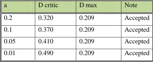
Table 10. Smirnov-Kolmogorof test for Log Pearson Type III

0.2 0.320 0.124 Accepted

0.1 0.370 0.124 Accepted

0.05 0.410 0.124 Accepted

0.01 0.490 0.124 Accepted

(11)

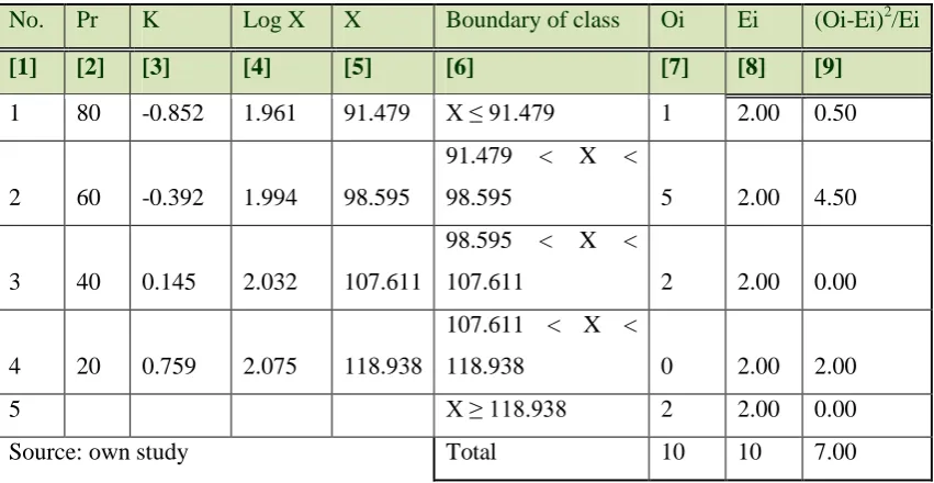
Table 11. Chi-square test for Log Pearson Type III

No. Pr K Log X X Boundary of class Oi Ei (Oi-Ei)2/Ei

[1] [2] [3] [4] [5] [6] [7] [8] [9]

1 80 -0.852 1.961 91.479 X ≤ 91.479 1 2.00 0.50

2 60 -0.392 1.994 98.595

91.479 < X <

98.595 5 2.00 4.50

3 40 0.145 2.032 107.611

98.595 < X <

107.611 2 2.00 0.00

4 20 0.759 2.075 118.938

107.611 < X <

118.938 0 2.00 2.00

5 X ≥ 118.938 2 2.00 0.00

G = 1+ 3,322 log n = 1 + 3,322 log 10 = 5

dk = k - (P + 1) = 7-(2+1)= 4

If X2 calculated >X2 table, it means that the distribution is not suitable

3.3.4. Metode Gumbel

Table 12 presents the analysis and the result of design rainfall by using the Gumbel method. However, Table 13 and

14 present the testing of goodness of fit each for Smirnov-Kolmogorof Test and chi-square test.

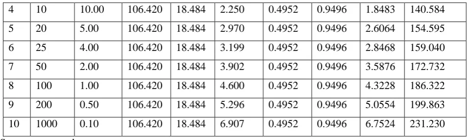
Table12. Design rainfall by using Gumbel method

No Tr Probabil

ity R mean

Deviati

on

standar

d

Variant

reductio

n

Mean

reductio

n

Variant

standard

deviatio

n

K Design rainfall (X)

(year) (%) (mm) (Sd) (Yt) (Yn) (Sn) (mm)

[1] [2] [3] [4] [5] [6] [7] [8] [9] [10]

1 1.25 80.00 106.420 18.484 -0.476 0.4952 0.9496 -1.0226 87.518

2 2 50.00 106.420 18.484 0.367 0.4952 0.9496 -0.1355 103.915

(12)

5 20 5.00 106.420 18.484 2.970 0.4952 0.9496 2.6064 154.595

6 25 4.00 106.420 18.484 3.199 0.4952 0.9496 2.8468 159.040

7 50 2.00 106.420 18.484 3.902 0.4952 0.9496 3.5876 172.732

8 100 1.00 106.420 18.484 4.600 0.4952 0.9496 4.3228 186.322

9 200 0.50 106.420 18.484 5.296 0.4952 0.9496 5.0554 199.863

10 1000 0.10 106.420 18.484 6.907 0.4952 0.9496 6.7524 231.230

Source: own study

Table 13. Smirnov-Kolmogorof test for Gumbel method

0.2 0.320 0.153 Accepted

0.1 0.370 0.153 Accepted

0.05 0.410 0.153 Accepted

0.01 0.490 0.153 Accepted

Source: own study

Table 14. Chi-square test for Gumbel method

[1] [2] [3] [4] [5] [6] [7] [8]

1 80 -1.023 87.518 X ≤ 87.518 1 2.00 0.50

2 60 -0.431 98.449

87.518 < X <

98.449 4 2.00 2.00

3 40 0.262 111.269

98.449 < X <

111.269 3 2.00 0.50

4 20 1.058 125.977

111.269 < X <

125.977 0 2.00 2.00

5 X ≥ 125.977 2 2.00 0.00

G = 1+ 3,322 log n = 1 + 3,322 log 10 = 5

dk = k - (P + 1) = 5-(2+1)= 2

(13)

Based on the analysis as above, the arithmetic mean for analyzing the area rainfall in the Lesti sub-watershed is

suitable. However, for the frequency distribution analysis for calculating the design rainfall, the suitable method is

Gumbel. It is due to the testing of goodness of fit is accepted for the Smirnov-Kolmogiorof test as well as the

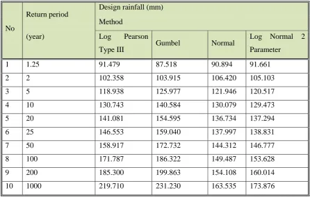
chi-square test. Table 15 presents the recapitulation of design rainfall by using the methods of Normal, Log

Normal, Log Pearson Type III, and Gumbel and Table 16 present the recapitulation of testing of goodness of fit for

the four methods.

Table 15. The recapitulation of design rainfall result in the Lesti sub-watershed

No

Return period Design rainfall (mm) Method

(year) Log Pearson

Type III Gumbel Normal

Log Normal 2

Parameter

1 1.25 91.479 87.518 90.894 91.661

2 2 102.358 103.915 106.420 105.103

3 5 118.938 125.977 121.946 120.517

4 10 130.743 140.584 130.079 129.473

5 20 141.081 154.595 136.734 137.294

6 25 146.553 159.040 137.997 138.831

7 50 158.917 172.732 144.312 146.777

8 100 171.787 186.322 149.487 153.628

9 200 185.300 199.863 154.108 160.014

10 1000 219.710 231.230 163.535 173.876

Source: own study

Table 16. Recapitulation of testing of goodness of fit

No

Testing of goodness

of fit

Design rainfall (mm)

Method

Method Log Pearson

Type III Gumbel Normal

Log Normal 2

Parameter

1 Smirnov-Kolmogorof Accepted Accepted Accepted Accepted

2 Chi-Square Non accepted Accepted

Non

accepted Non accepted

(14)

1. Y., Li; W., Cai; and E.P., Campbell. 2004. Statistical modelling of extreme rainfall in Southwest Western

Australia. Journal of Climate, Vol. 18, 852-863.

2. Nicholls, N., and B. Lavery. 1992. Australian rainfall trends during the twentieth century. Int. J. Climatol.,

12, 153–163.

3. Smith, I. N., B. C. Bates, E. P. Campbell, and N. Nicholls. 2000. Cause and predictability of decadal

variations. Indian Ocean Climate Initiative Research Rep. November 2000, 9–13.

4. National Research Council. 1998. Global Energy and Water Cycle Experiment (GEWEX)

Continental-Scale International Project (GCIP): A Review of Progress and Opportunities, p. 93, National

Academy Press, Washington, D.C.

5. Krajewski, W. F., G. J. Ciach, and E. Habib. 2003. An analysis of small scale rainfall variability in different

climatic regimes. Hydrol. Sci. J., 48, 151– 162.

6. Villarini, G.; V. Mandapaka, Pradeep; F. Krajewski, Witold; and Robert J., Moore. 2008. Rainfall and

sampling uncertainties: A rain gauge perspective. Journal of Geophysical Research, Vol. 113, D11102

doi:10.1029/2007JD009214

7. Hamada, A. 2014. Regional characteristics of extreme rainfall extracted from TRMM PR measurements.

Journal of Climate, Vol. 27, 8151-8169

8. Aguilar, E., and Coauthors. 2005. Changes in precipitation and temperature extremes in Central America

and northern South America, 1961–2003. J. Geophys. Res., 110, D23107, doi:10.1029/2005JD006119.

9. Alexander, L. V., and Coauthors. 2006. Global observed changes in daily climate extremes of temperature

and precipitation. J. Geophys. Res., 111, D05109, doi:10.1029/2005JD006290.

10. Allen, M. R., and W. J. Ingram. 2002. Constraints on future changes in climate and the hydrologic cycle.

Nature, 419, 224–232, doi:10.1038/nature01092.

11. Houze, R. A., Jr. 2012. Orographic effects on precipitating clouds. Rev. Geophys., 50, RG1001,

doi:10.1029/2011RG000365.

12. Lin, Y.-L., S.Chiao, T.-A.Wang, M. L. Kaplan, and R. P.Weglarz. 2001. Some common ingredients for

heavy orographic rainfall. Wea. Forecasting, 16, 633–660,

doi:10.1175/1520-0434(2001)016,0633:SCIFHO.2.0.CO;2.

13. Monaghan, A. J., D. L. Rife, J. O. Pinto, C. A. Davis, and J. R. Hannan. 2010. Global precipitation

extremes associated with diurnally varying low-level jets. J. Climate, 23, 5065–5084,

doi:10.1175/2010JCLI3515.1.

14. Lau, K.-M., Y. P. Zhou, and H.-T. Wu, 2008: Have tropical cyclones been feeding more extreme rainfall?

J. Geophys. Res., 113, D23113, doi:10.1029/2008JD009963.

15. SOSRODARSONO S., TAKEDA K. (eds.) 2003. Hidrologi untuk Pengairan [Hydrology for watering].