Optimization of the input space for deep learning data analysis
in HEP.
Andrei Chernoded2,, Lev Dudko1,, Georgi Vorotnikov1,, Petr Volkov1,, Dmitri Ovchinnikov2,†,MaximPerfilov1,‡, andArtemShporin2,§
1Lomonosov Moscow State University, Skobeltsyn Institute of Nuclear Physics (SINP MSU), 1(2), Leninskie gory, GSP-1, Moscow 119991, Russian Federation
2Faculty of Physics, Lomonosov Moscow State University, Leninskie Gory, Moscow 119991, Russian Fed-eration
Abstract.Deep learning neural network technique is one of the most efficient and general
approach of multivariate data analysis of the collider experiments. The important step of such analysis is the optimization of the input space for multivariate technique. In the article we propose the general recipe how to find the general set of low-level observables sensitive for the differences in the collider hard processes.
Introduction
Many high energy physics tasks in the collider experiments require modern efficient techniques to reach the desired sensitivity. The rather general scheme of HEP data analysis contains the distin-guishing of some rare physics process from overwhelming background processes. Neural network technique (NN) is one of the most popular and efficient multivariate method to analyze multidimen-sional space of observables which helps to increase the sensitivity of the experiment. Possible op-timizations of the set of high-level observables for multivariate analysis were considered previously and general recipe was formulated [1, 2] based on the analysis of Feynman diagrams which contribute to signal and background processes. The novel approach of deep learning neural network (DNN) be-comes more popular and more efficient in some cases [3]. The main advantage of DNN is the ability to operate with raw low-level unpreprocessed data and recognize the necessary features during the training stage. Unfortunately, the checks of naive implementation of DNN with low-level observ-ables, such as four momenta of final particles, do not demonstrate desired efficiency. The matter of this article is to propose the general recipe to find the set of low-level observables for DNN analysis of the collider hard processes.
e-mail: [email protected] e-mail: [email protected] e-mail: [email protected] e-mail: [email protected]
1 Check of the conception
Training of the NN usually means an approximation of some function. The classification tasks can be considered as an approximation of the multidimensional function which match the class of input vector to the desired output of NN for this class. What types of functions can be approximated in this manner? The question can be traced historically to the 13th mathematical problem formulated by David Hilbert [4]. It can be formulated in the following way: "can every continuous function of three variables be expressed as a composition of finitely many continuous functions of two variables?". The general answer has been given by Andrey Kolomogorov and Vladimir Arnold [5] in the Kol-mogorov–Arnold representation theorem: "every multivariate continuous function can be represented as a superposition of continuous functions of one variable". Based on this theorem, one can conclude that the methods developed for NN training, potentially can approximate all continuous multivariate functions. In reality, if we consider the standard form of perceptronyi =σ(nj=1wi jxj+θi) the only
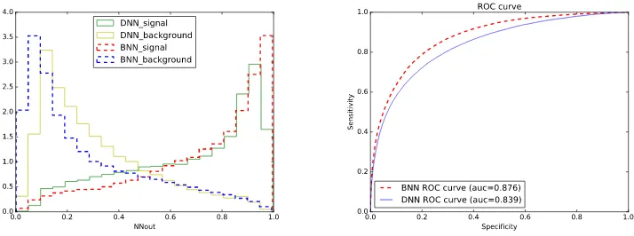
nonlinear part is the activation functionσ(). For the most simple case, if we take very popular acti-vation function ReLU (σ(x)=xforx>0 andσ(x)=0 forx<0), the whole NN with many layers and perceptrons is the linear combination of the input variables. One need to understand what type of functions we consider in High energy physics to describe the properties of the collider hard processes and how to describe the input space in most general and efficient way. In the collider physics one formulate the properties based on four-momenta of the final particles. The reasonable way is to take all possible four-momenta of all final particles as the input vector for the DNN analysis and during the training DNN resolves the sensitive features. We can try to check the hypothesis and find the general low-level observables for the DNN implementation. For the DNN training we use Tensorflow [7] and Keras [8] software. For the criteria of the efficiency one can use more simple, but efficient Bayesian neural networks (BNN) [9, 10] with only one hidden layer. The set of high-level input variables for BNN is very specific for the particular physics processes and is highly optimized based on the method mentioned above [2]. As an example of the physics task we consider distinguishing of the t-channel single-top-quark production from pair-top-quark production processes. The task is not trivial, but is already considered many times in the past [6]. The set of high-level input variables for the cross-check of the efficiency is the same as in the analysis of CMS collaboration [11]. The Monte-Carlo simula-tion has been performed in CompHEP package [12]. At the first step of the check we compare the efficiency of BNN and DNN with the same set of high-level input variables. The comparison is shown in the Fig. 1. The left plot demonstrates output of DNN and BNN for the signal and background pro-cesses. The right plot demonstrates ROC (Receiver Operating Characteristics) curve which is usually used to demonstrate the efficiency. The efficiency is higher if the Area Under the Curve (AUC) is higher.
1 Check of the conception
Training of the NN usually means an approximation of some function. The classification tasks can be considered as an approximation of the multidimensional function which match the class of input vector to the desired output of NN for this class. What types of functions can be approximated in this manner? The question can be traced historically to the 13th mathematical problem formulated by David Hilbert [4]. It can be formulated in the following way: "can every continuous function of three variables be expressed as a composition of finitely many continuous functions of two variables?". The general answer has been given by Andrey Kolomogorov and Vladimir Arnold [5] in the Kol-mogorov–Arnold representation theorem: "every multivariate continuous function can be represented as a superposition of continuous functions of one variable". Based on this theorem, one can conclude that the methods developed for NN training, potentially can approximate all continuous multivariate functions. In reality, if we consider the standard form of perceptronyi=σ(nj=1wi jxj+θi) the only
nonlinear part is the activation functionσ(). For the most simple case, if we take very popular acti-vation function ReLU (σ(x)=xforx>0 andσ(x)=0 forx<0), the whole NN with many layers and perceptrons is the linear combination of the input variables. One need to understand what type of functions we consider in High energy physics to describe the properties of the collider hard processes and how to describe the input space in most general and efficient way. In the collider physics one formulate the properties based on four-momenta of the final particles. The reasonable way is to take all possible four-momenta of all final particles as the input vector for the DNN analysis and during the training DNN resolves the sensitive features. We can try to check the hypothesis and find the general low-level observables for the DNN implementation. For the DNN training we use Tensorflow [7] and Keras [8] software. For the criteria of the efficiency one can use more simple, but efficient Bayesian neural networks (BNN) [9, 10] with only one hidden layer. The set of high-level input variables for BNN is very specific for the particular physics processes and is highly optimized based on the method mentioned above [2]. As an example of the physics task we consider distinguishing of the t-channel single-top-quark production from pair-top-quark production processes. The task is not trivial, but is already considered many times in the past [6]. The set of high-level input variables for the cross-check of the efficiency is the same as in the analysis of CMS collaboration [11]. The Monte-Carlo simula-tion has been performed in CompHEP package [12]. At the first step of the check we compare the efficiency of BNN and DNN with the same set of high-level input variables. The comparison is shown in the Fig. 1. The left plot demonstrates output of DNN and BNN for the signal and background pro-cesses. The right plot demonstrates ROC (Receiver Operating Characteristics) curve which is usually used to demonstrate the efficiency. The efficiency is higher if the Area Under the Curve (AUC) is higher.
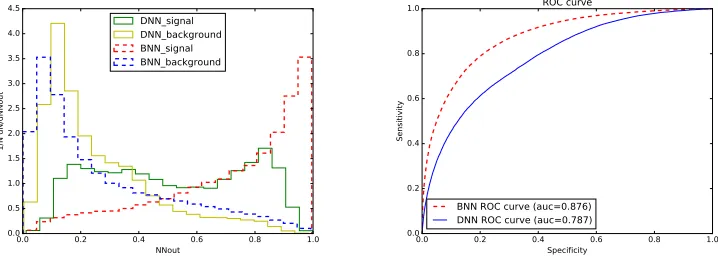
In the Fig. 1 one can see the same efficiency of the BNN and DNN with one hidden layer, for the same set of high-level variables. We can conclude that both of the methods provide the same sensitiv-ity for the same input vector. But, the DNN method is able to prepare very large networks with many hidden layers and analyze raw low-level features. At the second step of the cross-check we compare the same benchmark BNN with DNN trained on naive set of low-level variables with four-momenta of the final particles, which was mentioned above. The corresponding comparison is shown in Fig. 2. In the Fig. 2 one can see that DNN trained with complete set of four-momenta of final particles pro-vides worse result than benchmark BNN trained with optimized high-level variables. Such behavior demonstrate that one need to understand deeper the function which has to be approximated and the raw input vector to describe the input space for DNN.
Figure 1: The comparison of the BNN and DNN trained on the same set of high-level input variables. BNN and DNN have one hidden layer. The left plot demonstrates output of DNN and BNN for the signal and background processes. The right plot demonstrates ROC curve.
Figure 2: The comparison of benchmark BNN with DNN trained on the naive set of input variables with four-momenta of the final particles. DNN has three hidden layers. The left plot demonstrates output of DNN and BNN for the signal and background processes. The right plot demonstrates ROC curve.
2 Formulation of the general recipe to form the input space for DNN
analysis of HEP scattering processes.
The main properties of the collider hard process, e.g. differential cross sections, are proportional to the squared matrix element of the particular hard process. The concrete form of the matrix elements are different, but in all cases this is the function of scalar products of four-momenta or Mandelstam Lorentz-invariant variables. For example [13], the form of the squared matrix element for the sim-ple s-channel single top production processud¯ → tb¯, in terms of scalar products of four-momenta (pu,pb,pd,pt):
|M|2=Vtb2Vud2(gW)4 (pupb)(pdpt)
( ˆs−m2
W)2+γ2Wm2W
or it can be rewritten in terms of Mandelstam variables using (pupb)=−tˆ/2 , (pdpt) =(Mt2−tˆ)/2,
(pdpb)=−uˆ/2 , (pupt)=(M2t −uˆ)/2 andMtis the top quark mass:
|M|2=Vtb2Vud2(gW)4
ˆ
t(ˆt−M2 t)
( ˆs−m2
W)2+γ2Wm2W
. (2)
From the textbooks one knows that for the 2→ nscattering processes there are 3n−4 independent components and minimal set of observables can construct the complete basis. We would suggest that the correct approach is to take scalar products of four-momenta as the input space for the DNN analysis. The comparison of such approach with benchmark BNN is shown in the Fig. 3. The Fig. 3
Figure 3: The comparison of benchmark BNN with DNN trained on the scalar-products of four-momenta of the final particles as the set of input variables. DNN has three hidden layers. The left plot demonstrates output of DNN and BNN for the signal and background processes. The right plot demonstrates ROC curve.
demonstrates significantly worse efficiency of DNN trained with scalar products of four-momenta in comparison with benchmark BNN. The reason is simple in this case, matrix element depends on scalar products of four-momenta not only of the final particles, but also the four-momenta of the initial particles, which we can not reconstruct for the hadron colliders. For the mass-less particles thet = (pfinal−pinitial)2 variables can be rewritten in the following form [2]: ˆti,f = −√seˆ YpTfe−|yf|,
where ˆsis invariant mass of the final particles,Y = 12ln(p+pz
p−pz) is pseudorapidity of the center mass
of the system,PTf andyf are transverse momenta and pseudorapidity of the final particle. Therefore,
or it can be rewritten in terms of Mandelstam variables using (pupb)=−tˆ/2 , (pdpt)=(Mt2−tˆ)/2,
(pdpb)=−uˆ/2 , (pupt)=(Mt2−uˆ)/2 andMtis the top quark mass:
|M|2=Vtb2Vud2(gW)4
ˆ
t(ˆt−M2 t)
( ˆs−m2
W)2+γW2m2W
. (2)
From the textbooks one knows that for the 2→ nscattering processes there are 3n−4 independent components and minimal set of observables can construct the complete basis. We would suggest that the correct approach is to take scalar products of four-momenta as the input space for the DNN analysis. The comparison of such approach with benchmark BNN is shown in the Fig. 3. The Fig. 3
Figure 3: The comparison of benchmark BNN with DNN trained on the scalar-products of four-momenta of the final particles as the set of input variables. DNN has three hidden layers. The left plot demonstrates output of DNN and BNN for the signal and background processes. The right plot demonstrates ROC curve.
demonstrates significantly worse efficiency of DNN trained with scalar products of four-momenta in comparison with benchmark BNN. The reason is simple in this case, matrix element depends on scalar products of four-momenta not only of the final particles, but also the four-momenta of the initial particles, which we can not reconstruct for the hadron colliders. For the mass-less particles thet = (pfinal−pinitial)2 variables can be rewritten in the following form [2]: ˆti,f = −√seˆ YpTfe−|yf|,
where ˆsis invariant mass of the final particles,Y = 12ln(p+pz
p−pz) is pseudorapidity of the center mass
of the system,PTf andyf are transverse momenta and pseudorapidity of the final particle. Therefore,
we can try to add four-momenta of the final particles in additional to the scalar products of the final particles as the more complete basis to describe the input space for DNN analysis. The comparison is shown in Fig. 4 where benchmark BNN is compared with DNN trained on the set of scalar products and four-momenta of the final particles. The Fig. 4 demonstrates very similar performance of the DNN trained with rather general set of low-level variables and benchmark BNN trained with highly optimized set of high-level variables. At the last step of our comparison we can try to apply DNN in the space of low- and high-level variables and check is there some improvements in the sensitivity. Such comparison with benchmark BNN is shown in the Fig. 5. The Fig. 5 demonstrates almost the same DNN performance as in Fig. 4 for the DNN trained with general set of low-level variables, not a significant improvement in the first case can be associated with an approximate translation of the four-momenta of the initial particles, where optimized set of high-level variables add more information in comparison with the general low-level set of variables.
Figure 4: The comparison of benchmark BNN with DNN trained on the scalar-products of four-momenta and four-four-momenta of the final particles as the set of input variables. DNN has five hidden layers. The left plot demonstrates output of DNN and BNN for the signal and background processes. The right plot demonstrates ROC curve.
Figure 5: The comparison of the benchmark BNN and DNN trained on the complete set of low- and high-level input variables. DNN has three hidden layers. The left plot demonstrates output of DNN and BNN for the signal and background processes. The right plot demonstrates ROC curve.
Conclusion
of such general recipe has been demonstrated by the comparison with well investigated and highly optimized set of high-level variables constructed for the real data analysis in CMS experiment [11].
Acknowledgments
The work was supported by grant 16-12-10280 of Russian Science Foundation.
References
[1] E. Boos and L. Dudko, “Optimized neural networks to search for Higgs boson production at the Tevatron,” Nucl. Instrum. Meth. A502, 486 (2003) doi:10.1016/S0168-9002(03)00477-7 [hep-ph/0302088].
[2] Boos, E.E., Bunichev, V.E., Dudko, L.V. et al. Phys. Atom. Nuclei (2008) 71 388. https://doi.org/10.1134/S1063778808020191 “Method of “optimum observables” and implemen-tation of neural networks in physics investigations”
[3] P. Baldi, P. Sadowski and D. Whiteson, “Searching for Exotic Particles in High-Energy Physics with Deep Learning,” Nature Commun. 5, 4308 (2014) doi:10.1038/ncomms5308 [arXiv:1402.4735 [hep-ph]].
[4] Hilbert, David (1902). "Mathematical problems". Bulletin of the American Mathematical Society. 8: 461–462.; D. Hilbert, "Über die Gleichung neunten Grades", Math. Ann.97(1927), 243–250; https://en.wikipedia.org/wiki/Hilbert%27s_thirteenth_problem
[5] Andrey Kolmogorov, "On the representation of continuous functions of several variables by su-perpositions of continuous functions of a smaller number of variables", Proceedings of the USSR Academy of Sciences, 108 (1956), pp. 179–182; English translation: Amer. Math. Soc. Transl., 17 (1961), pp. 369–373.; Vladimir Arnold, "On functions of three variables", Proceedings of the USSR Academy of Sciences, 114 (1957), pp. 679–681; English translation: Amer. Math. Soc. Transl., 28 (1963), pp. 51–54.
[6] B. Abbottet al.[D0 Collaboration], “Neural networks for analysis of top quark production,” hep-ex/9907041.
[7] M. Abadiet al., “TensorFlow: Large-Scale Machine Learning on Heterogeneous Distributed Sys-tems,” arXiv:1603.04467 [cs.DC]. Software available from tensorflow.org.
[8] Chollet, François and others, “Keras” 2015 Software available from keras.io
[9] Radford M. N., "Bayesian learning for neural networks", 1994, Dept. of Statis-tics and Dept. of Computer Science, University of Toronto", ISBN 0-387-94724-8, http://www.cs.utoronto.ca/~radford/bnn.book.html
[10] Radford M. Neal, "Software for flexible Bayesian modeling and Markov chain sampling", 2004, Dept. of Statistics and Dept. of Computer Science, University of Toronto, 2004-11-10, http://www.cs.toronto.edu/~radford/fbm.software.html
[11] V. Khachatryanet al.[CMS Collaboration], “Search for anomalous Wtb couplings and flavour-changing neutral currents in t-channel single top quark production in pp collisions at √s=7 and 8 TeV,” JHEP1702, 028 (2017) doi:10.1007/JHEP02(2017)028 [arXiv:1610.03545 [hep-ex]]. [12] E. Boos et al. [CompHEP Collaboration], Nucl. Instrum. Meth. A 534, 250 (2004)
doi:10.1016/j.nima.2004.07.096 [hep-ph/0403113].
[13] E. Boos, V. Bunichev, L. Dudko and M. Perfilov, “Interference betweenWandWin single-top