Phase-dependent effects in bichromatic high-order harmonic generation
C. Figueira de Morisson Faria,1D. B. Milosˇevic´,2,*and G. G. Paulus3 1
Max Planck Institut fu¨r Physik komplexer Systeme, No¨thnitzer Strasse 38, 01187 Dresden, Germany 2Max-Born-Institut fu¨r nichtlineare Optik und Kurzzeitsspektroskopie, Max-Born-Strasse 2A, 12489 Berlin, Germany
3Max Planck Institut fu¨r Quantenoptik, Hans-Kopfermann Strasse 1, 85748 Garching, Germany 共Received 4 November 1999; published 17 May 2000兲
We address high-order harmonic generation with linearly polarized bichromatic fields, concentrating on a modulation in the harmonic yield as a function of the relative phase between the two field components, and on an offset phase shift of this modulation for neighboring cutoff harmonics. These effects have been recently observed in experiments where the relative phase between the two driving fields was controlled. Using the three-step model and the fully numerical solution of the time-dependent Schro¨dinger equation, we discuss the phase-dependent modulation and show that the offset phase is inherent to a particular set of semiclassical trajectories for the returning electron. These trajectories are identified using classical arguments and isolated by means of the saddle-point method, which allows a detailed investigation of their interference. Thus, by adding a second driving field whose amplitude lies within an adequate parameter range, one is able to single out a set of trajectories according to its behavior with respect to the relative phase. This effect is already present at the the single-atom-response level.
PACS number共s兲: 42.50.Hz, 32.80.Rm, 32.80.Qk, 42.65.Ky
I. INTRODUCTION
The emission spectrum of a gaseous sample exposed to a strong laser field covers a long frequency range with har-monics of roughly the same intensities, the so-called ‘‘pla-teau,’’ followed by an abrupt decrease in the harmonic yield, the so-called ‘‘cutoff’’ 关1兴. A very intuitive and successful description of these features is given by the so-called ‘‘three-step model’’关2–5兴: an electron leaves the atom through tun-neling or multiphoton ionization, propagates in the con-tinuum and, depending on its emission time, may be driven back by the field and recombine with its parent ion, such that harmonic radiation up to the extreme ultraviolet 共XUV兲 re-gime is emitted. Within this picture, the cutoff corresponds to the maximum kinetic energy of the electron upon return and is given, for monochromatic fields, by ⍀max⫽兩0兩 ⫹3.17Up, where 兩0兩 and Up are the ionization potential and the ponderomotive energy, respectively. This model de-scribes existing experiments in some respect even quantita-tively and has also been successfully tested against other theoretical methods, such as the fully numerical solution of the time-dependent Schro¨dinger equation关6兴, with strikingly similar spectral and temporal profiles, for monochromatic 关7–10兴, bichromatic 关11,12兴, and short-pulsed laser fields 关13兴. One of the strongest experimental evidences that the physical picture of semiclassical electron trajectories is cor-rect has been provided recently in Ref. 关14兴. Therein, the trajectories in question have been isolated using effects re-lated to the propagation of the harmonic radiation in the gaseous medium. These experiments have also shown that one can in principle manipulate the harmonic spectra by ex-ploiting particular characteristics of harmonics
correspond-ing to specific trajectories, for instance their different sensi-tivity to propagation and phase matching.
For a similar reason, i.e., the possibility of coherent con-trol of XUV emission, high-order harmonic generation with bichromatic fields has attracted a lot of attention in the past few years, both theoretically 关11,12,15–18兴and experimen-tally关19–21兴. In fact, by changing the shape of the bichro-matic field, one can in principle manipulate the electron mo-tion in the continuum, suppressing or enhancing particular groups of harmonics. Already for the simplest case, namely a linearly polarized laser field, one can strongly influence the harmonic spectra by varying the field amplitudes, and, in the case of commensurate frequencies, the relative phase be-tween the driving fields. In previous publications, we have shown that the introduction of a second driving field may result in several maximal- and minimal-energy trajectories for the returning electron, which correspond to cutoffs in the emission spectra 关11,12兴, such that the plateau presents a much more complex structure in the bichromatic than in the monochromatic case.
Several parameters determine the prominence of a cutoff in the spectrum: the total field strength at the electron emis-sion time t0, the excursion time of the electron in the con-tinuum, and the interference between different semiclassical trajectories. The first parameter is of extreme importance, since the electron leaves the atom with a probability related to the quasistatic ionization rate 关22兴, exp关⫺C/兩E(t0)兩兴. A very effective way to control the field strength 兩E(t0)兩 is changing the relative phase between the laser field compo-nents of different frequencies. For instance, in 关11兴we pro-vide an example for which the harmonic yield decreases con-siderably for a chosen interval of the relative phase where this parameter was particularly weak. Also the interference between the semiclassical trajectories depends very strongly on the relative phase. In principle, slight changes in may radically alter this interference pattern, so that variations of *On leave from the Faculty of Science and Mathematics,
orders of magnitude in the harmonic yield are observed, for isolated groups of harmonics关12兴.
Experimentally, this phase control has been achieved re-cently for high-order harmonic generation in helium and ar-gon, using a linearly polarized ⫺2 field of comparable intensities关21兴. The intensity of the low-frequency field was kept fixed, whereas the high-frequency field and the relative phase were varied. The wavelength of the low-frequency field was approximately ⫽800 nm and intensities of the order of 1015 W/cm2have been used. In this experiment, the harmonic yield as a function of the relative phase, with all other parameters kept constant, exhibits the following main features:共i兲The intensity of the cutoff harmonics is modu-lated. A shift of 2 in the relative phase between the and 2 fields corresponds to two periods of the modulation of each harmonic. 共ii兲 The modulation itself shows an offset phase shift as the harmonic order is varied: if the modulation of the nth harmonic presents a maximum as a function of for a certain phase 0, then this maximum will be slightly shifted, i.e., it will be at0⫹␦ for the (n⫹1)th harmonic. These effects are present within a relatively broad range of intensity ratios I2/I 关21兴. The theoretical modeling of these experiments reproduces these findings reasonably well, however, without providing a physical explanation for either the modulation or its phase shift. In关21兴, as a first approxi-mation, the cutoff energy was taken as the monochromatic value ⍀max⫽兩0兩⫹3.17Up and the ponderomotive energy
was related to the low-frequency field only, such that Upwas
chosen as Up⫽I/42.
In this paper we give a simple explanation of these effects based on the analysis of classical trajectories, within the three-step model and single-atom-response framework. In particular, we isolate the relevant semiclassical trajectories using the saddle-point method, computing the harmonic spectra as the interference between these trajectories. Besides the experimental facts, the conclusions drawn from the clas-sical and semiclasclas-sical computations are checked against the results from a fully numerical solution of the time-dependent Schro¨dinger equation for a one-dimensional model atom with a single bound state, whose energy corresponds to the argon ionization potential. We use atomic units throughout. The paper is outlined as follows: in Sec. II we present our theoretical methods, namely the classical or ‘‘simple-man’’ model 共Sec. II A兲, the saddle-point method 共Sec. II B兲, and the time-dependent Schro¨dinger equation共Sec. II C兲. In Sec. III we present and discuss our results and in Sec. IV we state our conclusions.
II. THEORY
A. Classical model
In order to determine the emission and return times and the kinetic energy of the returning electron, we take the nu-merical solution of the classical equations of motion of an electron in the field
Eជ共t兲⫽eជˆx关E01sin共t兲⫹E02sin共2t⫹兲兴, 共1兲
where denotes the relative phase and E0ithe amplitude of
each driving wave. Since all the ensuing motion takes place along the polarization axis, the problem can be treated one dimensionally. At the initial time t0, the electron leaves the atom with zero velocity, propagates in the continuum under the influence of the laser field only, and returns to the site of its release at a later time t1, such that x(t1)⫽0. During the process, canonical momentum is conserved. Therefore, the kinetic energy of the electron upon return is given by
Ekin共t1,t0兲⫽ 1
2关A共t1兲⫺A共t0兲兴
2, 共2兲
with A(t) being the vector potential, related to the external field by E(t)⫽⫺dA(t)/dt. This yields a harmonic energy
⍀H⫽兩0兩⫹Ekin共t1,t0兲 共3兲
by the recombination to the ground state. Following this simple picture, the kinetic energy Ekin(t0,t1), the emission time t0, and the return time t1can be associated to a classical trajectory for the returning electron. The cutoff frequencies are determined by the condition that the kinetic energy is extremal upon return, namely dEkin(t1,t0)/dt1⫽0. The emission and return times are connected by the revisiting condition. We use this model either for a single electron, varying the emission time t0 within a cycle T⫽2/of the low-frequency driving field and calculating Ekin(t1,t0), which is subsequently plotted as a function of the emission and return times, or we consider an ensemble of electrons whose emission time is varied randomly from 0 to T. In this latter case, we select electrons that satisfy the condition
x(t1)⫽0 within a particular set of harmonic energies, given by Eq.共3兲, and we look at electron counts as functions of the relative phase. The contribution of each single electron is weighed with the quasistatic ionization rate关22,23兴
⌫⬃
冋
2 5/2兩0兩3/2 兩E共t0兲兩
册
冑2/兩0兩⫺1
exp
冋
⫺2 5/2兩0兩3/2
3兩E共t0兲兩
册
. 共4兲The first and the second procedures have been used in 关11,12兴and关24兴, respectively.
B. Strong-field approximation and saddle-point method
The classical model discussed in Sec. II A provides useful information concerning the cutoff law and the emission and return times for the electron. However, it does not account for the quantum interference between two or more possible trajectories for the returning electron, which lead to well-structured harmonic spectra 关25–27兴. For this purpose, we use a closely related quantum-mechanical approach: the strong-field approximation 共SFA兲 theory of high-order har-monic generation关3,5,18兴.
Within the SFA, the nth harmonic strength is defined as the Fourier component of the time-dependent dipole关3,5,18兴
Dn⫽⫺i
冕
0
Tdt
T e
int
冕
0
⬁ d
冉
2i
冊
3/2
F共ps;t,兲
F共ps;t,兲⫽
具
0兩x兩ps⫺A共t兲典具
ps⫺A共t⫺兲兩xE共t⫺兲兩0典
, 共5兲where ⫽t⫺t0 is the excursion time of the electron in the continuum, 兩0
典
is the atomic ground state, and ps ⫽兰t⫺dt⬘
A(t⬘
)/is the stationary momentum, for which thequasiclassical action
S共p;t,兲⫽
冕
t⫺ t
dt
⬘
再
12关p⫺A共t
⬘
兲兴2⫹
冏
0冏
冎
共6兲satisfies the conditionⵜpS( p;t,)⫽0. The harmonic yield is
proportional to n4兩Dn兩2. The double integral in Eq. 共5兲 can
be solved using the saddle-point method 共SPM兲, with the result 关25,26兴
Dn⬀
兺
s s⫺3/2关
det共2Ss兲兴⫺1/2Fsexp关i共nts⫺Ss兲兴, 共7兲
where det(2Ss) denotes the determinant of the 2⫻2 matrix
formed by the second derivatives of the action with respect to t0 and t at p⫽ps. For hydrogenlike atoms the product of
the dipole matrix element Fs can be approximated by (n
⫺兩0兩)1/2/n3. The sum in Eq. 共7兲 extends over all relevant saddle points which satisfy the conditions关18兴
1
2关ps⫺A共t0兲兴
2⫽⫺兩0兩,
1
2关ps⫺A共t兲兴 2⫺1
2关ps⫺A共t0兲兴
2⫽n. 共8兲
We will show in Sec. III that a good approximation for Dn
can be obtained taking into account only four complex solu-tions for pairs (t,t0).
C. Time-dependent Schro¨dinger equation
As our point of reference, we take the one-dimensional time-dependent Schro¨dinger equation 共TDSE兲 关6兴 for a single electron subject to a binding potential and a bichro-matic field共1兲. A one-dimensional共1D兲model is not so de-manding as a full three-dimensional computation and still describes results for linearly polarized fields adequately in qualitative terms 关28兴. In the velocity gauge, this equation reads
id
dt兩共t兲
典
⫽冋
p22⫹V共x兲⫺pA共t兲
册
兩共t兲典
. 共9兲 The quadratic term in A(t) was removed by a unitary trans-formation. The binding potential was chosenV共x兲⫽⫺1.1 exp共⫺x2/1.21兲, 共10兲
such that the model atom has a single field-free bound state with energy0⫽⫺0.58 a.u. According to the experimental conditions the lower frequency of the driving field is taken as ⫽0.057 a.u. The power spectra are computed from the
time-dependent dipole acceleration x¨(t)⫽
具
(t)兩 ⫺dV(x)/dx⫹E(t)兩(t)典
关29兴.III. RESULTS
A. Upper and lower cutoff branches
For a monochromatic field, the maximum of Ekin(t1,t0) is at the well-known value 3.17Up, and the semiclassical
tra-jectories originating the cutoff obey a T/2 periodicity. For bichromatic fields, however, this property is maintained only if the higher frequency is an odd multiple of the lower fre-quency. This is clear, since, for these types of fields, A(t ⫹T/2)⫽⫾A(t). On the other hand, if the ratio between the
higher and the lower frequency is even, this symmetry is broken. Since the kinetic energy of the electron depends on
A(t) according to Eq. 共2兲, this results in a splitting of the cutoff energy into an upper and a lower branch named, re-spectively, ⍀uand⍀l. This feature can be seen in detail as
function of the field strength ratio E02/E01⫽, for⫽0, in a previous publication 关12兴. These branches behave in strik-ingly different ways with respect to the relative phase. The energy of the upper cutoff branch practically does not vary with this parameter, whereas the lower branch is strongly phase dependent. These features are present for intensity ra-tios smaller than or of the order of I2⫺⫽I2/I⯝0.2. For higher intensity ratios there is a much more complicated pat-tern for the cutoff energies as functions of the phase. For instance, the case of equally strong driving waves has been discussed in关11,12兴.
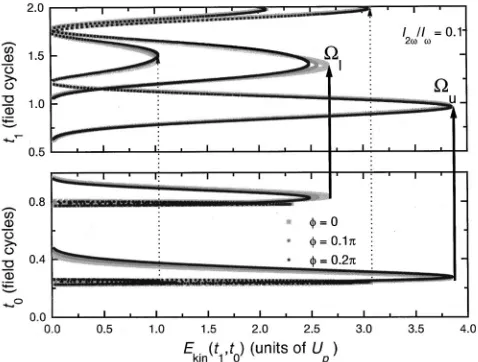
An example is shown in Fig. 1, where Ekin(t1,t0) is plot-ted as a function of the emission and return times, for 0 ⭐⭐0.2 and ⫽0.32. This corresponds to an intensity ratio I2⫺⫽I2/I⫽0.1. Each point „t0,t1,Ekin(t0,t1)… in the curves shown fulfills the revisiting condition x(t1)⫽0, thus characterizing a trajectory for the returning electron. Given an emission time t0 on the curve in the lower part of the figure, the return time t1 in the corresponding curve in the upper part of the figure is determined by the intersection of the latter curve with a perpendicular line starting from the lower curve at t0. The return energy can be read from the ordinate of the graph. The local energy maxima give the cutoffs, and each of these maximal-energy trajectories splits into two, corresponding to a shorter and a longer excursion time for the electron in the continuum. Thus, for a given
Ekin(t1,t0), there may be many possible trajectories for the returning electron. Quantum mechanically, the probability amplitudes related to the electron following each of these trajectories interfere. The cutoff branches ⍀u and ⍀l are
marked with thick solid arrows. For this field-strength ratio, the energy of the upper cutoff branch is at roughly ⍀u
⫽3.8Up, whereas ⍀l varies from 2.6Up to 2.3Up for the
phase interval in question. In the figure and in the results that follow, the kinetic energy is displayed in units of the pon-deromotive energy calculated for the whole field, given by
Up⫽兺nUpn⫽E012/42⫹E 02
lower and upper branches are given by, respectively, (t1l,t0l)⯝(0.85T,1.4T) and (t1u,t0u)⯝(0.35T,0.9T). Their precise values depend on the relative phase . For the pa-rameters considered, the remaining cutoffs, marked with dashed arrows, do not play an important role in the present problem, either for being too near the ionization threshold or due to very long excursion times for the electron, which results in a pronounced wave packet spreading.
A more detailed description of the process above can be obtained using the complex time formalism 关25,26兴. SPM equations 共8兲, for 兩0兩⫽0, have only complex solutions t0 and t1⬅t. These solutions, for 0⭐t0⭐T and 0⭐t1⫺t0⭐T,
are presented in Fig. 2. On the left-hand side we present the imaginary part of t0 共scaled to the optical cycle T) as a function of the real part of t0, and, similarly, on the right-hand side we present solutions for t1. The numbers on the curves correspond to the harmonic order n for which solu-tions were found, for the same intensity ratio as in the pre-vious figure and E01⫽0.1 a.u. It is evident that the solutions
S1 and S2 correspond to the lower cutoff branch, while the solutions S3 and S4correspond to the upper one. The cutoffs appear for values of n which correspond to the closest points of the curves S1 and S2 共or S3 and S4). The physical mean-ing of the imaginary parts of times t0 and t1 is connected with the probability that the process in question occurs. This follows from Eq. 共7兲 because, for one particular trajectory, the logarithm of the harmonic yield is proportional to Im关nt1⫺S( ps,t1,)兴. Beyond the points denoted by n ⫽50 for the solutions S1 and S2 共and also by n⫽65 for S3
and S4) the imaginary parts increase in absolute value. If these imaginary parts are negative, Eq. 共7兲gives low emis-sion rates, and, consequently, the position of the cutoff. Oth-erwise, they lead to an exponential increase in the harmonic yield. More precisely, in the application of Eq. 共7兲 beyond the denoted cutoff points, one of the solutions S1 and S2 (S3 and S4) should be discarded as unphysical. Therefore, for
n⬎65 only one trajectory contributes to the harmonic spec-tra. For 50⭐n⭐65 three trajectories contribute, while for n ⬍50 all trajectories contribute to the harmonic yield.
B. Harmonic spectra
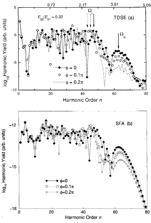
The importance of each set of trajectories in the harmonic spectra can be inferred from the quantum-mechanical com-putation. The lower branch is considerably more prominent in the spectra, whereas the most energetic cutoff appears only as a small shoulder. Thus, the ‘‘cutoff’’ seen experi-mentally corresponds to the strongly phase-dependent set of trajectories. Figures 3 and 4 present some of these spectra, for field strengths E01⫽0.1 a.u. and E02⫽0.032 a.u., which are within the experimental parameter range. For these pa-rameters and 0⭐⭐0.2, the upper and lower branches of ⍀maxcorrespond to the harmonic frequencies⍀u⫽63 and
43.1⬍⍀l⬍47.4, respectively. Both cutoff branches are
indicated in the figure.
Figures 3共a兲and 3共b兲present results obtained solving the TDSE 共see Sec. II C兲 and the SFA 共see Sec. II B兲, respec-tively. Apart from a very good agreement between both re-sults for lower and upper cutoff branches, one observes an energy displacement for the lower branch as is varied, whereas the energy of the upper cutoff branch remains prac-tically inaltered. These results are in perfect agreement with the predictions of Sec. III A obtained using the classical model.
FIG. 1. Classical emission and return times for an electron in a bichromatic field given by Eq.共1兲as functions of its kinetic energy upon return, Ekin(t1,t0), for various relative phases 0⭐⭐0.2.
The vertical axes in the upper and lower parts correspond, respec-tively, to the emission and return times, given by t0 and t1. The
field strengths are chosen such that E02/E01⫽0.32, the kinetic
en-ergy is given in units of the ponderomotive enen-ergy, and the emis-sion and return times in units of the period of the low-frequency field, T⫽2/. The cutoff energies are marked with arrows con-necting both parts of the figure. The thick solid arrows corresponds to the upper and lower cutoff branches and the remaining cutoff energies are indicated by dashed arrows. The influence of the bind-ing potential was neglected.
FIG. 2. Complex solutions t0 and t1of the SPM equations共8兲
for a hydrogenlike atomic potential with兩0兩⫽0.58 a.u., the same
laser field parameters as in Fig. 1, and the relative phase⫽0. Four solutions 共denoted by S1, S2, S3, and S4) are obtained for the
In Fig. 4 we compare the SFA results to the spectra ob-tained using the saddle-point method. The SPM results are obtained taking only four relevant complex solutions for the times t0 and t1 in Eq. 共7兲 共see Fig. 2兲. The results agree qualitatively with the TDSE and SFA results for n⬎30. This shows that the main contribution to the harmonic yield near both cutoff branches comes from the four complex trajecto-ries which have been explicitly discussed in Sec. III A.
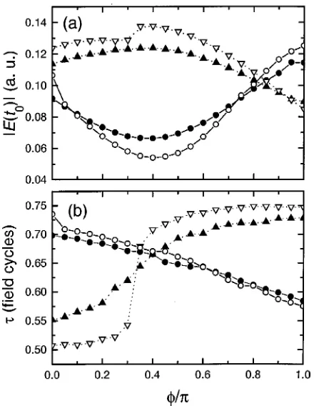
A more detailed investigation of the field strength兩E(t0)兩 at the emission time explains part of the features observed in Figs. 3 and 4. Figure 5共a兲 displays this parameter for the lower and upper branches, for intensity ratios I2⫺⫽0.1 and 0.2. We show only the behavior for 0⭐⭐, since the semiclassical trajectories obey a period of with respect to the phase, due to the symmetry E(t,⫹)⫽⫺E(t
⫺T/2,). This property is discussed in detail in 关12,30兴. From the figure it is clear that for a wide phase interval, namely for 0⭐⭐0.8, the lower branch presents a
consid-erably larger field at the emission time, such that its promi-nence in the spectrum is justified. This promipromi-nence decreases for the phase interval where both fields are comparable. An-other important parameter is the excursion time of the elec-tron in the continuum: the shorter the excursion time, the less
FIG. 3. Harmonic yields as functions of the harmonic order n calculated using the TDSE 关part共a兲兴and the strong-field approxi-mation关part共b兲兴, for the same bichromatic field as in the previous figures, with E01⫽0.1 a.u. and relative phase 0⭐⭐0.2. The
numbers on the upper edge of part共a兲give the corresponding ki-netic energy Ekin(t1,t0) in units of the ponderomotive energy Up.
The upper and lower cutoff branches are indicated by thick arrows in part共a兲. For the phases⫽0,⫽0.1, and⫽0.2, the cutoff
⍀lis indicated by a solid, dashed, and dotted arrow, respectively.
FIG. 4. Harmonic yields calculated with the saddle-point method 共solid lines兲 compared to the strong-field approximation
共stars connected by dashed lines兲for the same bichromatic field and ionization potential as in Fig. 3, for共a兲⫽0,共b兲⫽0.1, and共c兲
important wave packet spreading. For both cutoff branches, these times are comparable and vary with the relative phase . For phases smaller than⯝0.4, the excursion time for the lower branch is slightly shorter than that of the upper branch. For the remaining phases, this pattern is reversed. This can be seen in Fig. 5共b兲, for the same intensity ratios as in the previous part of the figure. Thus, this does not appear to play a significant role in this case.
C. Modulation and its phase shift
For both lower and upper cutoff branches, the TDSE com-putation yields a modulation for the harmonic intensities as functions of the relative phase , which is periodic in . Thisperiodicity is due to the symmetry in E(t) mentioned in Sec. III B.
In order to study the offset phase shift, we investigate this modulation for consecutive harmonics near and slightly be-yond the lower and upper cutoff branches. Figure 6共a兲shows this variation for harmonics near ⍀u obtained from the
quantum-mechanical computation, compared with the quasi-static rate for E(t0u). The obvious coincidence between them indicates that for the upper branch the harmonic yield is de-termined by the quasistatic ionization rate, i.e., by the prob-ability per unit time that the ‘‘first step’’ takes place. This is related to the fact that these harmonics are mainly
deter-mined by a single cutoff trajectory whose energy is almost independent of the relative phase. Thus, other mechanisms that may influence the harmonic yield and produce a modu-lation, such as pronounced interference effects or significant variations in the harmonic intensities due to a shift in the cutoff energy, do not play a significant role.
On the other hand, for the lower cutoff branch the TDSE computation clearly shows a phase shift of the modulation for neighboring harmonics, which qualitatively corresponds to the feature reported in 关21兴. This phase shift is shown in Fig. 6共b兲, where the harmonic intensity is plotted as a func-tion of the relative phase, for harmonics slightly beyond⍀l,
namely at 兩0兩⫹3Up. It is strongly related to the variation
of the cutoff energy with . As a particular harmonic ap-proaches or gets further in energy from⍀l, there is either an
increase or a decrease in the harmonic yield. For a given phase, this intensity variation depends on the harmonic or-der, since different harmonics are unequally distant from the lower cutoff branch. Thus, neighboring harmonics present similar intensities for slightly different phases. For energies
FIG. 5. Field strength兩E(t0)兩at the emission time关part共a兲兴and
excursion times⫽t1⫺t0关part共b兲兴, for the upper and lower cutoff
branches, for intensity ratios I2⫺⫽0.1 共filled symbols兲, and I2⫺⫽0.2共open symbols兲, as functions of the relative phase.
The triangles connected by dotted lines and the circles connected by solid lines correspond to the lower cutoff ⍀land the upper cutoff
⍀u, respectively.
FIG. 6. Harmonic yield from the TDSE computation for neigh-boring cutoff harmonics compared to the quasistatic ionization rate, as functions of the relative phase, for a driving field as in Fig. 3. Parts 共a兲 and共b兲refer to the cutoff branches⍀uand ⍀l,
respec-tively. Part 共a兲 displays the harmonics⍀⫽63, ⍀⫽64, and⍀
⫽65, whose energies are slightly larger than兩0兩⫹3.8Up, while
part 共b兲 shows the harmonics ⍀⫽52, ⍀⫽53, and ⍀⫽54, with energies around 兩0兩⫹3Up 共slightly beyond the cutoff ⍀l).
The thick lines in the figure give the formula
⫺25/2兩
lower than or roughly at ⍀l, there is also a pronounced
interference structure superposed to the global behavior, which sometimes disguises this phase shift. This is not sur-prising since, in this energy region,⍀lsplits into two sets of
trajectories for the returning electron which are temporally and energetically very close. For energies of the order of 兩0兩⫹3Up, these interference effects are practically absent.
Figure 6共b兲also shows that the modulation observed does not follow the quasistatic ionization rate, given by the thick line in the figure. In fact, the modulation observed is a con-sequence of other physical mechanisms in addition to the tunneling process at the emission time, namely the energy variation of the lower cutoff branch and the interference be-tween trajectories belonging to the lower and upper branches. As already discussed, the phase dependence of⍀l
is responsible for the phase shift of the modulation. Another example of its influence on the harmonic yield is a pro-nounced intensity drop seen in Fig. 6共b兲, which occurs for ⯝0.25. For this phase, the energy difference between the group of harmonics chosen and the cutoff ⍀l is most
pro-nounced.
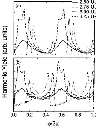
The offset phase shift is also present within the simple-man model, as described in Sec. II A for an electron en-semble with randomly distributed start times 0⭐t0⭐T. This
confirms the classical origin of this effect since, due to the strong phase dependence of ⍀l, as is varied different
amounts of electrons come from⍀land⍀u. Since electrons
with slightly different Ekin(t1,t0) are unequally distant in energy from the lower branch, the corresponding electron counts are also expected to be phase shifted with respect to each other. Figure 7 shows these counts as functions of the relative phase for different electron kinetic energies, which include contributions for one or both cutoff branches, de-pending on the phase in question. A more detailed behavior of⍀lwith the phase will be discussed below. In Fig. 7共a兲we
take into account the ionization rate given by Eq. 共4兲, whereas in Fig. 7共b兲we consider a constant ionization rate. The main difference between them is that, in Fig. 7共a兲, one of the two sets of peaks observed in Fig. 7共b兲 is strongly suppressed. Thus,兩E(t0)兩 influences the modulation, but not its phase shift, only selecting the trajectories for which the field strengths at the electron start times are particularly strong.
The precise behavior of ⍀l and ⍀u with respect to the
phase as calculated with the simple-man model is shown in Fig. 8 for several intensity ratios. Each point in the figure corresponds to an extremal kinetic energy for the returning electron. Figure 8共a兲confirms that the cutoff energies⍀uare
very weakly influenced by the phase. The most important feature observed in the figure is the displacement of ⍀u to-wards higher energies for an increasing intensity of the high-frequency wave. This effect has been discussed in a previous paper 关12兴. On the other hand, for the cutoff ⍀l Fig. 8共b兲
shows a strong energy variation as is changed. An inter-esting feature is the energy minimum mentioned above at 0.25 for intensity ratios of the order of or smaller than
I2/I⫽0.2. For stronger 2fields, the cutoff⍀lsplits into
two, such that the interpretation of the results concerning the
phase-dependent modulation becomes considerably more complicated.
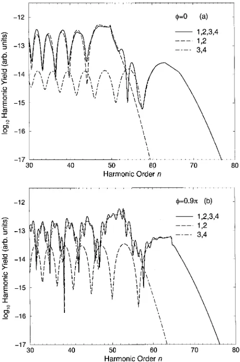
The interference between the lower and upper cutoff branches plays only a secondary role in this modulation be-ing, however, present for phases in the interval 0.5⭐ ⭐, for which E(t0l) and E(t0u) are comparable and the excursion timeu⫽t1u⫺t0u is shorter than that of the lower branch. Some information concerning these interferences can be obtained using the saddle-point method. In Fig. 9 we present the spectra resulting from isolated pairs of trajecto-ries, compared to the results obtained taking into account all four relevant trajectories. Figure 9共a兲 displays these results for ⫽0, clearly showing that the lower cutoff branch is almost entirely determined by the trajectories S1 and S2. For ⫽0.9 关Fig. 9共b兲兴, on the other hand, one clearly sees an interference pattern in the harmonics of the lower cutoff branch, originated by the trajectories S3 and S4.
IV. CONCLUSIONS
We investigate high-order harmonic generation with bichromatic ⫺2 fields, giving a physical interpretation for the phase shift of the modulation observed experimen-tally for neighboring cutoff harmonics关21兴. Using the three-step model and the fully numerical solution of the time-dependent Schro¨dinger equation, we show that this feature is determined by the phase dependence of a set of semiclassical trajectories for the returning electron. With the introduction of the high-frequency driving wave, the cutoff for the mono-chromatic case splits into two branches, which exhibit
differ-FIG. 7. Harmonic yields for various harmonic energies between
⍀land⍀uas functions of the relative phasecalculated from the
classical model. In part共a兲the quasistatic ionization rate given by Eq.共4兲and in part共b兲a field-independent ionization rate was used. The calculation was performed with an ensemble of 5⫻107 elec-trons and randomly distributed start times t0 and phases . The
kinetic energy at the return time t1was identified with the photon
ent behavior with respect to the relative phase between the two driving fields. While the cutoff energy of the upper branch does not vary considerably with the phase, the cutoff energy of the lower branch is strongly sensitive to this pa-rameter, giving rise to the phase shift of the modulation. Thus, using a two-color field, one can separate and identify a set of semiclassical trajectories already for a single atom, whereas for a monochromatic field, this is only possible us-ing propagation effects of the harmonic radiation in the gas-eous sample关14兴.
Using the saddle-point method, we are also able to make precise statements on how the interference between various trajectories influence the harmonic spectra, and reproduce the full quantum-mechanical results obtained with the TDSE for the harmonics close to the upper and lower cutoff branches with astonishing precision. We show that in the high plateau and cutoff regions, the harmonic intensities are well de-scribed by four interfering semiclassical trajectories for the returning electron. In particular, a single trajectory is respon-sible for the upper cutoff branch, whereas the lower branch is the result of the interference of three different trajectories.
Another noteworthy feature is the difference of orders of magnitude between the harmonic yields of the upper and lower branches. This is a direct consequence of a stronger field at the electron emission time for the cutoff ⍀l and
therefore an interesting example of how groups of harmonics can be enhanced or suppressed by manipulating兩E(t0)兩. Fur-thermore, the fact that the upper cutoff branch extends to
energies higher than⍀max⫽兩0兩⫹3.17Up, but that the lower
cutoff branch is more prominent in the spectra sheds some light into several apparently conflicting theoretical and ex-perimental findings for high-order harmonic generation in bichromatic fields. In a large number of theoretical investi-gations, an extension of the plateau towards higher energies is observed, for ⫺2 关11,12,16兴 and ⫺3 关17兴 fields, whereas other theoretical and experimental studies yield a shorter 关18,19,21兴 plateau in comparison to the monochro-matic cutoff energy ⍀max. Our results suggest that these studies refer either to the upper or to the lower cutoff branch, so that no contradiction exists. In particular, a double plateau was observed in 关18兴for a bichromatic driving field of fre-quencies and 2, and the result found for the cutoff en-ergy is in very good agreement with⍀l.
We also propose an explanation for the phase modulation observed in the harmonic yield for upper and lower cutoff branches. For the upper branch, this modulation is entirely
FIG. 8. Cutoff energy as a function of the phasefor the upper
关part共a兲兴and lower关part共b兲兴cutoff branches, given in terms of the ponderomotive energy Up. The solid squares, open circles, crosses,
and diamonds correspond to the intensity ratios I2⫺⫽0.1, I2⫺⫽0.2, I2⫺⫽0.3, and I2⫺⫽0.4, respectively. For
inten-sity ratios larger than 0.2, there is a splitting of the lower cutoff⍀l.
FIG. 9. Harmonic yields calculated using the SPM equations共7兲 and 共8兲 for a hydrogenlike atomic potential with兩0兩⫽0.58 a.u.,
determined by the quasistatic tunneling rate, whereas for the lower branch, it appears to be the combination of three main physical mechanisms, namely the field strength 兩E(t0l)兩 at the emission time of the electron in the continuum, the en-ergy variation of the cutoff enen-ergy⍀lwith the relative phase
, and the interference between the upper and lower cutoff branches, which plays a role when the fields at the emission time兩E(t0l)兩and兩E(t0u)兩are comparable for both branches. Finally, we would like to comment on the cutoff mea-sured in 关21兴 for helium, whose energy was taken near the 15th harmonic of the low-frequency field. This strong reduc-tion in the cutoff energy was related to poor phase-matching conditions 关31兴. For this gas, however, the ionization
poten-tial is roughly兩0兩⯝0.9 a.u., which corresponds to approxi-mately⍀⫽15, with the frequency of the laser used being ⫽0.057 a.u. In this frequency region, the atomic internal structure strongly influences the harmonic spectra, such that the application or interpretation of the results in terms of the three-step model is questionable关10,32兴.
ACKNOWLEDGMENTS
Discussions with W. Becker, R. Kopold, M. Do¨rr, E. Cormier, and M. Lewenstein are gratefully acknowledged. D. B. Milosˇevic´ is supported by the Alexander von Hum-boldt Foundation.
关1兴For a recent review, consult P. Salie`res, A. L’Huillier, Ph. Antoine, and M. Lewenstein, Adv. At., Mol., Opt. Phys. 41, 83
共1999兲.
关2兴M. Yu. Kuchiev, Pis’ma Zh. E´ ksp. Teor. Fiz. 45, 319 共1987兲
关JETP Lett. 45, 404 共1987兲兴; K. C. Kulander, K. J. Schafer, and J. L. Krause, in Super-Intense Laser-Atom Physics, Vol. 316 of NATO Advanced Science Institute Series, Series B:
Physics, edited by B. Piraux, A. L’Huillier, and K. Rza¸z˙ewski 共Plenum, New York, 1993兲; P. B. Corkum, Phys. Rev. Lett.
71, 1994共1993兲.
关3兴M. Lewenstein, Ph. Balcou, M. Yu. Ivanov, A. L’Huillier, and P. B. Corkum, Phys. Rev. A 49, 2117共1994兲.
关4兴W. Becker, S. Long, and J. K. McIver, Phys. Rev. A 41, 4112
共1990兲; 50, 1540共1994兲.
关5兴W. Becker, A. Lohr, M. Kleber, and M. Lewenstein, Phys. Rev. A 56, 645共1997兲.
关6兴See, e.g., M. Protopapas, C. H. Keitel, and P. L. Knight, Rep. Prog. Phys. 60, 389共1997兲, and references therein.
关7兴S. C. Rae, K. Burnett, and J. Cooper, Phys. Rev. A 50, 3438
共1994兲; R. Taı¨eb, A. Maquet, Ph. Antoine, and B. Piraux, in
Super Intense Laser-Atom Physics IV, Proceedings of the
NATO Advanced Workshop on SILAP IV, Moscow, Russia, 1995, edited by H. G. Muller and M. V. Fedorov 共Kluwer, Dordrecht, 1996兲, p. 445.
关8兴C. Figueira de Morisson Faria, M. Do¨rr, and W. Sandner, Phys. Rev. A 55, 3961共1997兲.
关9兴Ph. Antoine, B. Piraux, D. B. Milosˇevic´, and M. Gajda, Laser Phys. 7, 594共1997兲.
关10兴C. Figueira de Morisson Faria, M. Do¨rr, and W. Sandner, Phys. Rev. A 58, 2990共1998兲.
关11兴C. Figueira de Morisson Faria, M. Do¨rr, W. Becker, and W. Sandner, Phys. Rev. A 60, 1377共1999兲.
关12兴C. Figueira de Morisson Faria, W. Becker, M. Do¨rr, and W. Sandner, Laser Phys. 9, 388共1999兲.
关13兴A. de Bohan, Ph. Antoine, D. B. Milosˇevic´, and B. Piraux, Phys. Rev. Lett. 81, 1837 共1998兲; A. de Bohan, D. B. Milosˇevic´, G. L. Kamta, and B. Piraux, Laser Phys. 9, 175
共1999兲.
关14兴M. Bellini, C. Lynga˚, A. Tozzi, M. B. Gaarde, T. W. Ha¨nsch, A. L’Huillier, and C.-G. Wahlstro¨m, Phys. Rev. Lett. 81, 297
共1998兲; M. B. Gaarde, F. Salin, E. Constant, Ph. Balcou, K. J.
Schafer, K. C. Kulander, and A. L’Huillier, Phys. Rev. A 59, 1367共1999兲.
关15兴M. Protopapas, P. L. Knight, and K. Burnett, Phys. Rev. A 49, 1945 共1994兲; T. Zuo, A. D. Bandrauk, M. Ivanov, and P. B. Corkum, ibid. 51, 3991共1995兲; S. Long, W. Becker, and J. K. McIver, ibid. 52, 2262 共1995兲; D. M. Telnov, J. Wang, and S.-I. Chu, ibid. 52, 3988共1995兲; W.-C. Liu and C. W. Clark,
ibid. 53, 3582共1996兲; M. Protopapas and P. L. Knight, J. Phys. B 28, 4459共1995兲; M. B. Gaarde, A. L’Huillier, and M. Le-wenstein, Phys. Rev. A 54, 4236 共1996兲; S. Varro´ and F. Ehlotzky, ibid. 56, 2439 共1997兲; A. D. Bandrauk, S. Chelkowski, H. Yu, and E. Constant, ibid. 56, R2537共1997兲; Ph. Antoine, D. B. Milosˇevic´, A. L’Huillier, M. B. Gaarde, P. Salie`res, and M. Lewenstein, ibid. 56, 4960 共1997兲; J. Z. Ka-min´ski and F. Ehlotzky, J. Phys. B 30, 5729 共1997兲; X.-M. Tong and S.-I. Chu, Phys. Rev. A 58, R2656共1998兲; F. Giam-manco and P. Ceccherini, Laser Phys. 8, 593 共1998兲; Ph. V. Ignatovich, V. T. Platonenko, and V. V. Strelkov, J. Opt. Soc. Am. B 16, 435 共1999兲; S. Bivona, R. Burlon, and C. Leone,
ibid. 16, 986 共1999兲; W. Becker, B. N. Chichkov, and B. Wellegehausen, Phys. Rev. A 60, 1721共1999兲; V. Averbukh, O. E. Alon, and N. Moiseyev, ibid. 60, 2585共1999兲.
关16兴C. A. Ullrich, S. Erhard, and E. K. U. Gross, in Super Intense
Laser Atom Physics IV共Ref.关7兴兲, p. 477.
关17兴M. Protopapas, A. Sanpera, P. L. Knight, and K. Burnett, Phys. Rev. A 52, R2527 共1995兲; A. Sanpera, J. B. Watson, M. Le-wenstein, and K. Burnett, ibid. 54, 4320共1996兲.
关18兴D. B. Milosˇevic´ and B. Piraux, Phys. Rev. A 54, 1522共1996兲. We use the opportunity to mention a misprint in this reference: on the left-hand side in the first equation in Eq.共22兲it should beជ2(t⫺) and notជ2(t).
关19兴M. D. Perry and J. K. Crane, Phys. Rev. A 48, R4051共1993兲.
关21兴U. Andiel, G. D. Tsakiris, E. Cormier, and K. Witte, Europhys. Lett. 47, 42共1999兲.
关22兴See, e.g., L. D. Landau and E. M. Lifshitz, Quantum
Mechan-ics共Pergamon, Oxford, 1977兲.
关23兴M. V. Ammosov, N. B. Delone, and V. P. Krainov, Zh. E´ ksp. Teor. Fiz. 91, 2008共1986兲 关Sov. Phys. JETP 64, 1191共1986兲兴.
关24兴G. G. Paulus, W. Becker, and H. Walther, Phys. Rev. A 52, 4043共1995兲.
关25兴M. Lewenstein, P. Salie`res, and A. L’Huillier, Phys. Rev. A
52, 4747共1995兲.
关26兴R. Kopold, D. B. Milosˇevic´, and W. Becker, Phys. Rev. Lett.
84, 17共2000兲.
关27兴G. van de Sand and J. M. Rost, Phys. Rev. Lett. 83, 524
共1999兲.
关28兴In a one-dimensional computation, interference effects related to trajectories with long excursion times are overenhanced, since transversal wave-packet spreading is absent. In Eqs.共5兲 and共7兲, this neglect would give an exponent⫺1/2 instead of
⫺3/2 in the prefactor.
关29兴K. Burnett, V. C. Reed, J. Cooper, and P. L. Knight, Phys. Rev. A 45, 3347 共1992兲; J. L. Krause, K. Schafer, and K. Kulander, ibid. 45, 4998共1992兲.
关30兴K. J. Schafer and K. C. Kulander, Phys. Rev. A 45, 8026
共1992兲.
关31兴See, e.g., A. L’Huillier, M. Lewenstein, P. Salie`res, P. Balcou,
M. Yu. Ivanov, J. Larsson, and C.-G. Wahlstro¨m, Phys. Rev. A
48, R3433共1993兲; C.-G. Wahlstro¨m, J. Larsson, A. Persson, T. Starczewski, S. Svanberg, P. Salie`res, Ph. Balcou, and A. L’Huillier, ibid. 48, 4709 共1993兲; P. Salie´res, A. L’Huillier, and M. Lewenstein, Phys. Rev. Lett. 74, 3776共1995兲; J. Peat-ross, M. V. Fedorov, and K. C. Kulander, J. Opt. Soc. Am. B
12, 863 共1995兲; Ph. Antoine, M. B. Gaarde, P. Salie`res, B. Carre´, A. L’Huillier, and M. Lewenstein, in Proceedings of the
VIIth International Conference on Multiphoton Processes,
ed-ited by P. Lambropoulos and H. Walther 共IOP Publishing, Bristol, 1997兲, p. 142; J. Zhou, J. Peatross, M. M. Murnane, H. C. Kapteyn, and I. P. Christov, Phys. Rev. Lett. 76, 752
共1996兲; P. Salie`res, T. Ditmire, M. D. Perry, A. L’Huillier, and M. Lewenstein, J. Phys. B 29, 4771 共1996兲; Ph. Balcou, P. Salie´res, A. L’Huillier, and M. Lewenstein, Phys. Rev. A 55, 3204 共1997兲; I. P. Christov, M. M. Murnane, and H. C. Kapteyn, ibid. 57, R2285共1998兲; M. B. Gaarde, Ph. Antoine, A. L’Huillier, K. J. Schafer, and K. C. Kulander, ibid. 57, 4553
共1998兲.