Privacy Preservation in Spatial Database

(1)

Privacy Preservation in Spatial Database

Ranu Sahu

1

_{& Raghvendra Kumar}

2 1,2

Dept. of Computer Scienece & Engineering, LNCT Group of College, Jabalpur, MP, India [email protected]; [email protected]

Abstract:

The majority of existing algorithms do not warrant the elimination of all well known geographic dependences. The result is that the same associations represented in geographic database schemas are extracted by spatial association rule mining algorithms and presented to the user. The problem of mining spatial association rules from geographic databases requires at least three main steps: compute spatial relationships, generate frequent patterns, and extract association rules. The first step is the most effort demanding and time consuming task in the rule mining process, but has received little attention in the literature. The second and third steps have been considered the main problem in transactional association rule mining and have been addressed as two different problems: frequent pattern mining and association rule mining. Well known geographic dependences which generate well known patterns may appear in the three main steps of the spatial association rule mining process. Aiming to eliminate well known dependences and generate more interesting patterns, this thesis presents a framework with three main methods for mining frequent geographic patterns using knowledge constraints. Semantic knowledge is used to avoid the generation of patterns that are previously known as non-interesting. The first method reduces the input problem, and all well known dependences that can be eliminated without losing information are removed in data preprocessing. The second method eliminates combinations of pairs of geographic objects with dependences, during the frequent set generation. A third method presents a new approach to generate the global relationship between the attributes without disclosing their private information to other reason in the geographic areas.

Keywords: Data Mining; Distributed Data Mining; Association Rule Mining; Spatial Data Mining; Spatial Association Rules; Weka Tool.

1. Introduction

(2)

2. Spatial Data Mining

Spatialdescribes how objects fit together in space, either among the planets or down here on earth. Spatial data refers to all types of data objects or elements that are present in a geographical space or horizon. It enables the global finding and locating of individuals or devices anywhere in the world. Spatial data base is a database that is enhanced to store and access spatial data or data that defines a geometric space. These data are often associated with geographic locations and features, or constructed features like cities. Data on spatial databases are stored as coordinates, points, lines, polygons and topology. Some spatial databases handle more complex data like three-dimensional objects, topological coverage and linear networks. Spatialdata mining is the application of data mining to spatial models. In spatial data mining, analysts use geographical or spatial information to produce business intelligence or other results. This requires specific techniques and resources to get the geographical data into relevant and useful formats.

3. Proposed Work

Due to the increased demand for knowledge discovery in all industrial domains, it is necessary to store all the raw spatial data and to provide useful patterns with respective to the user needs. Generally, the storage of all raw data will be done in a database maintained by concerned organizations. Data mining techniques are available to retrieve useful information from large spatial database. Prediction and description are the two fundamental goals of data mining. To full fill these goals many spatial data mining techniques exists such as association rules, classification, clustering and so on. Among these, association rule has wide applications to discover interesting relationship among attributes in large spatial databases. Spatial association rule mining is used to find the rules which satisfy the user specified minimum support and minimum confidence. In the process of finding association rules, the set of frequent item sets are computed as the first step and then association rules are generated based on these frequent item sets.

In this process, we divided the entire region into the three different region and each having their spatial database SDB1, SDB2,…..SDBn and their own key values SK1,SK2,……..SKn, or Select N number of

region each having their own database SDB1, SDB2,…., SDBn . Each region calculates their frequent items set and support value.

Figure 5.1: Communication among three region and DM

Each region are arrange in ring architecture then find the partial support , Now the region 1 send their Partial Support (PS) value to region 2 and region 2 send their value to region 3 and this process continue

Region1

(3)

till region n and after that region n send their value to region 1. region 1 subtract all the Random number value from the Partial Support value and calculate their actual support, now region 1 broadcast the actual support value to the entire region present in the distributed environment.

o Proposed Algorithm:

Encryption Process

Step1: Take the Spatial Database

Step2: Convert into the horizontally partitioned distributed database (N Number of datasets) Step3: Calculate the support count of each database with the help of Weka Tool.

Step4: Calculate the support and confidence.

Support =

)

Confidence =

Step5: Calculate partial support and partial confidence.

Partial Support (PS) = X. Support - DB inimum Support

Partial Confidence (PC) = X. Confidence - DB Minimum Confidence

Step7: Add their own private key in all partial support and partial confidence.

Partial Support (PS) = X. support - DB minimum support Key

Partial Confidence (PC) = X. Confidence - DB Minimum Confidence

Step8: Divided the partial support and partial confidence into the three different values.

Step9: Converted partial support, partial confidence and partial lift values into the ASCII value and compute the matrix Y.

Step10: Take the transpose of the matrix (YT).

Step11: Convert ASCII code matrix (YT) into the binary format.

Step12: Consider our own secret key(X matrix) Step 13: Covert the X matrix into binary format Step 14: Perform Exclusive-or between X and Y.

Step15: The resultant matrix is the encrypted format of plain text stored into the associative memory. Setp16: The resultant matrix is sanded to the protocol initiator Server.

Decryption Process

Step 1: Consider the resultant matrix M

Step 2: Compute transpose of M matrix as MT matrix Step 3: Convert matrix MT into binary format

Step 4: Consider our own private key X

Step 5: Covert matrix X into binary number format Step 6: Perform exclusive-or operation between MT and X

Step 7: The resultant matrix is converted to the ASCII code and finally we have the original text.

(4)

Broadcast

Step9: After that the protocol initiator broadcast the results to all the database server admin presents in the distributed environments.

Flow Chart:

Spatial Database (SDB1, SDB2,……,SDBn)

Select the Regions

Calculate the frequent items

Support =

Confidence =

Partial Support (PS) = X. support – DB minimum support

Partial Confidence (PC) = X. Confidence - DB Minimum Confidence+Key

Send Data P1 P2 then P2 P3 then P3 P1

Global Support (GS) = ∑ ∑ ) Global Confidence (GC) = ∑ ∑ )

Figure: Flow Chart

Start

(5)

Design & Implementation

In this thesis, we considered the spatial database, spatial database represented in table 1, table2 and table

3, which is partitioned into the homogeneous environment, having same number of attributes. Table1: Spatial Database for Region 1

TID REFRENCE CITY SPATIAL OBJECTS

A B C D E F G

1 MUMBAI 1 1 1 1 1 0 1

2 CHENNAI 1 0 1 0 1 0 1

3 BENGALURU 1 1 1 1 0 1 0

4 HYDERABAD 1 0 0 0 1 0 0

5 KOLKATA 0 1 0 1 0 1 0

6 RAIPUR 0 0 1 0 0 0 1

7 CHANDIGARH 1 1 1 0 0 1 0

8 INDORE 1 0 1 0 1 0 1

9 COIMBATORE 0 1 0 1 0 1 0

10 PUNE 1 1 1 1 1 0 1

Table2: Spatial Database for Region 2

A B C D E F G

1 SURAT 1 0 0 1 0 1 1

2 AHMEDABAD 1 1 1 1 1 0 0

3 NASHIK 0 1 1 0 1 0 0

4 KOCHI 1 0 0 1 0 0 1

5 RAJKOT 0 1 1 0 1 0 0

6 GURGAON 1 1 0 1 0 1 1

7 JAIPUR 1 0 0 1 0 0 1

8 BHUBANESHWAR 1 1 1 1 1 0 1

9 VISAKHAPATNAM 1 0 0 1 0 0 1

(6)

Table3: Spatial Database for Region 3

A B C D E F G

1 SURAT 1 0 0 1 0 1 1

2 AHMEDABAD 1 1 1 1 1 0 0

3 NASHIK 0 1 1 0 1 0 0

4 KOCHI 1 0 0 1 0 0 1

5 RAJKOT 0 1 1 0 1 0 0

6 GURGAON 1 1 0 1 0 1 1

7 JAIPUR 1 0 0 1 0 0 1

8 BHUBANESHWAR 1 1 1 1 1 0 1

9 VISAKHAPATNAM 1 0 0 1 0 0 1

10 TRIVENDRUM 1 1 1 0 0 0 0

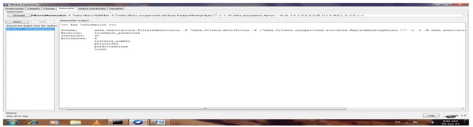
In this use the spatial database for region 1, it analyzed that database with the help of weka tool after applying the apriori algorithm, shows in below figure.

Figure: Shows analyzed dataset for the region 1

(7)

Figure: Shows analyzed dataset for the region 3

In this thesis, take the spatial database from three different regions, for analyzing the spatial database, consider the minimum support value is 40% and for providing the highest privacy to spatial database, it consider three different key numbers, whose value prospectively 1, 2 and 3. First each region calculated their support count by using the Apriori algorithm, then after that each region calculated their partial support by using the formula then after that added the key number and sanded to the next region head presented in the distributed environment, than after that the protocol initiator region will calculated their actual support, and broadcast it to all the region.

Region 1:

For the attribute AB, Key = 1, Support=0.40, Confidence=0.9

Partial Support (PS) = Mod (X. support - DB× Minimum Support + Key)=0.4-(10×0.4) + 1=2.6

Partial Confidence (PC) = Mod (X. Confidence - DB Minimum Confidence =0.9-10*0.6+1=4.1

Divided the partial support and confidence value into the three different values

PS1=1, PS2=1, PS3=0.60

PC1=2, PC2=2, PC3=0.1

Converted partial support and partial confidence values into the ASCII value and compute the matrix Y.

Y= [SOH SOH NULL]

Take the transpose of the matrix (YT)

YT=[

(8)

ASCII code matrix (YT) into the binary format

YT=[

]

Consider our own secret key(X matrix)

X1=[ ]

Covert the X matrix into binary format

X1=[

]

Perform Exclusive-or between X and Y

Z1=X Ex-OR YT=[

] [

] = [

]

Region 2:

Partial Support (PS) = Mod (X. support - DB× Minimum Support + Key) =0.4-(10×0.4) + 2=3.6

PS1=1, PS2=1, PS3=1.6

PC1=1, PC2=1, PC3=1.2

Y= [SOH SOH SOH ]

YT=[

]

(9)

YT=[

]

Consider our own secret key(X matrix)

X2=[ ]

X2=[

]

Z2=X Ex-OR YT=[

] [

] = [

]

Region 3:

Partial Support (PS) = Mod (X. support - DB× Minimum Support + Key)=0.4-(10×0.4) + 3=0.6

PS1=0.0, PS2=0.0, PS3=0.6

PC1=2, PC2=2, PC3=0.1

Y= [ NULL NULL NULL]

YT=[

]

ASCII code matrix (YT) into the binary format

YT=[

]

(10)

X3=[ ]

X3=[

]

Z3=X Ex-OR YT=[

] [

] = [

]

After the encryption, now the entire region sends their encrypted value with the key value, to the protocol

initiator region, then the protocol initiator region decrypted that value by using some of the decryption

steps that shown in the above algorithm. Perform the Ex-OR operation between the resulting matrix Z1

Ex-OR X1, Z2 Ex-OR X2 and Z3 Ex-OR X3. Then we have the matrix M1, M2 and M3, after that for

calculating the resulting matrix M, perform the Ex-OR operation between M1, M2 and M3.

M=M1 Ex-OR M2 Ex-OR M3= [

]

Then take the transpose of the resulting matrix

MT= [000 101 000] =0.5

After taking the transpose converted into the ASCII value and then, the value of the resulting matrix M is

same as the global support value, If the global support value greater than zero then it means that the,

attribute value, that has been taken is globally frequent attribute, it may be locally infrequent attribute. So

here, this thesis the calculated value of global support is greater than zero and it accepted as globally

frequent item.

Conclusion

We have seen that some of the discovered rules actually convey new knowledge, however the search for these “nuggets” requires a lot of tuning and efforts by the data analyst in order to constrain the search space properly and discard most of the obvious or totally useless patterns

(11)

References

[1] Boulicaut, J.F.; Jeudy, B. “Mining Free Itemsets Under Constraints”. In: International Database Engineering & Applications Symposium, Ideas, 2001, Washington Dc. Proceeding: Ieee Computer Society, 2001. P. 322-329.

[2] Brin, S.; Motwani, R.; Ullman, J.; Tsur, S. “Dynamic Itemset Counting And Implication Rules For Market Basket Data”. In: Acm Sigmod International Conference On Management Of Data, Sigmod, 1997, Tuscon. Proceedings: Acm Press, 1997. P. 255-264.

[3] Burdick, D.; Calimlim, M.; Gehrke, J. Mafia: “A Maximal Frequent Itemset Algorithm For Transactional Databases”. In: Ieee International Conference Data Engineering, Icde, 17., 2001, Heidelberg. Proceeding: Ieee Computer Society, 2001. P. 443-452.

[4] Chaves, M. S.; Silva, M. J.; Martins, B. “A Geographic Knowledge Base For Semanticweb Applications”. In: Brazilian Symposium On Databases, Sbbd, 20., 2005, Uberlândia. Proceedings: Ufu, 2005a. P.40-54.

[5] Chaves, M. S.; Silva, M. J.; Martins, B. “Gkb - Geographic Knowledge Base”. Lisboa: Di/Fcul, 2005.

[6] Chifosky, E.J.; Cross, J.H. “Reverse Engineering and Design Recovery”: A Taxonomy. Ieee Software, V.7, P.13-17, Jan. 1990.

[7] Clementini, E.; Di Felice, P.; Van Ostern, P. “A Small Set Of Formal Topological Relationships For End -User Interaction”. In: Abel, D; Ooi, B.C. (Ed.). Advances In Spatial

Databases: Springer-Verlag, 1993. P. 277-295.

[8] Clementini, E.; Di Felice, P.; Koperski, K. “Mining Multiple-Level Spatial Association Rules For Objects With A Broad Boundary”. Data & Knowledge Engineering, V.34, N.3, P.251-270, Sept. 2000.

[9] Cockcroft, S. A “Taxonomy Of Spatial Data Integrity Constraints”. Geo informatica, V.1, N.4, P.327-343, Dec. 1997.

[10] Ester, M. Et Al. “Spatial Data Mining: Database Primitives, Algorithms And Efficient Dbms Support”. Journal Of Data Mining And Knowledge Discovery, V.4, N.2-3, P.193-216, July 2000.

[11] Fayyad, U.; Piatetsky-Shapiro, G.; Smyth, P.” From Data Mining To Knowledge Discovery in Databases”. Ai Magazine, V.17, N.3. P.37-54, 1996.

[12] Fukuda, T. Et Al. “Mining Optimized Association Rules For Numeric Attributes” In: Acm Sigmod Symposium On Principles Of Database Systems, Pods, 15., 1996, Montreal. Proceeding: Acm Press, 1996. P.182-191.