Solving a Large-Scale Intertemporal Applied General Equilibrium Model

Full text

(1)CENTRE of POLICY STUDIESand the IMPACT PROJECT. Eleventh Floor Menzies Building PO Box 11E, Monash University Wellington Road CLAYTON Vic 3800 AUSTRALIA Telephone: (03) 9905 2398, (03) 9905 5112. from overseas: 61 3 9905 5112 or 61 3 9905 2398. Fax: (03) 9905 2426 e-mail web site. 61 3 9905 2426 [email protected]. http://www.monash.edu.au/policy/. Paper presented to the Australasian Meeting of the Econometric Society Monash University, July 1992. SOLVING A LARGE-SCALE INTERTEMPORAL APPLIED GENERAL EQUILIBRIUM MODEL by. Michael MALAKELLIS Industry Commission and. Monash University. Preliminary Working Paper Paper No. OP-74. July 1992. reissued August 2001. ISSN 1031 9034. ISBN 0 641 0209 0. The Centre of Policy Studies (CoPS) is a research centre at Monash University devoted to quantitative analysis of issues relevant to Australian economic policy..

(2) TABLE OF CONTENTS. Abstract. ii. 1. 2. 3.. 1 2 4. Introduction Dimensions and Structure of an Intertemporal CGE Model Solution Methods 3.1 3.2 3.3 3.4. Shooting Methods Relaxation Methods The Euler Method Newton-Raphson Method. 5 5 6 16. 4.. Modelling Sign Constraints. 20. 5.. Conclusion. 25. Bibliography. 26. LIST OF FIGURES AND DIAGRAMS Figure 1 Diagram Diagram Diagram Diagram. Schematic Representation of an Intertemporal Model 1 2 3 4. Diagram 5 Diagram 6 Diagram 7 Diagram 8. The Johansen or 1-Step Euler Method Euler Multistep Method Euler Method: Pathological Case 3-Step Euler Method: Initial Solution Not Known Exogenous Variables X Held Constant 3-Step Euler Method: Initial Solution Not Known Exogenous Variables X set to Forecast Values 3-Iteration Standard Newton-Raphson Method Euler Multistep Method from Initial Solutions with Newton-Raphson Error Correction Sign Constraints. i. 3 8 10 11 14 15 17 19 23.

(3) ABSTRACT Intertemporal Computable General Equilibrium (CGE) models have the potential to quantify the implications of sectoral and temporal linkages which are often crucial for understanding the effects of economic shocks. However, such models will prove to be of practical use for policy analysis only if accurate solutions can be obtained at reasonable cost. Often, the usefulness of intertemporal CGE models for policy analysis is diminished because the degree of economic detail incorporated is compromised in order to maintain computational tractability. The purpose of this paper is to describe how Euler's method may be used to solve large-scale intertemporal CGE models without compromising significantly on the type and degree of economic detail modelled.. In. particular, there is no need to restrict the number of costate variables (e.g., by assuming that capital stocks are homogeneous) nor to assume that the solution will always be interior.. ii.

(4) S OLVING A LARGE-SCALE INTERTEMPORAL APPLIED GENERAL EQUILIBRIUM MODEL by. Michael MALAKELLIS*. 1.. Introduction. A challenge of constructing an intertemporal Computable General Equilibrium (CGE) model is to keep it computationally tractable without compromising significantly on the type and degree of economic detail modelled. In a survey of Computable General Equilibrium (CGE) modelling, Manne (1985) observed that the dimensionality of intertemporal CGE models is typically reduced by adopting two assumptions; first, that "capital stocks are homogeneous (not specific to sectors or to regions), and that there are only a few types of capital stock variables" and second, that there are always interior solutions. The purpose of this paper is to describe how the Euler method, and variants thereof, may be used to solve a large-scale intertemporal CGE model without resorting to the dimensionality reduction schemes described above. A special case of Euler's method, the so-called Johansen (1960) method, has been used routinely to solve large-scale comparative static CGE models. The ORANI model of the Australian economy (see Dixon, Parmenter, Sutton and Vincent (1982) hereafter DPSV) is a prime example of this approach. A feature of the ORANI model that has made it widely used for policy analysis in Australia is the degree of economic detail which it incorporates. As will be explained in section 3.3, the Johansen method is computationally very simple. Consequently, constraints on model size and flexibility are less severe than for non-linear solution methods. As argued in DPSV (1982), the Johansen approach provides maximum scope for model modifications (e.g., changes in the equations, additions and deletions of equations, and respecification of the closure) without requiring that the solution algorithm be re-written. Together, the solution procedure used and the detail embodied in ORANI make it amenable to addressing a wide range of issues on a routine basis. An intertemporal CGE model that is as detailed as ORANI in terms of its description of the economy at any point in time has the potential to deal with issues involving both the composition of the economy (which has been the strength of comparative-static CGE models such as ORANI) and the allocation of resources over time. However a model of this size and complexity will only prove to be of practical use to the policy-maker only if accurate solutions can be obtained at reasonable cost.. *. Without implicating them in any remaining errors the author would like to thank Mark Horridge, Ken Pearson Alan Powell, Brian Parmenter and Matthew Peter for their helpful comments and assistance. 1.

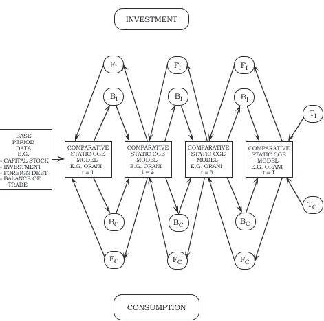
(5) 2. Michael Malakellis. The Johansen procedure is perhaps the fastest and least costly method for solving a large-scale comparative static CGE model. However there are two key reasons why this method may be inadequate for solving a large-scale intertemporal CGE model. First, solutions obtained via Johansen's procedure are of first order accuracy only and the approximation errors introduced cannot be controlled. DPSV (1982) argue that for most practical applications of ORANI, the Johansen method provides solutions which are free of significant approximation errors. However the ability to control the degree of approximation errors may be very important for an intertemporal CGE model. The second disadvantage of the Johansen method is that corner constraints are extremely difficult to model. The remainder of this paper is organised as follows: Section 2 provides an overview of the structure and dimensions of the class of intertemporal CGE models for which the solution method outlined in section 3 is targeted. Section 4 describes how sign constraints may be modelled using this preferred solution method and finally, section 5 presents some concluding remarks.. 2.. Dimensions and Structure of an Intertemporal CGE Model An intertemporal CGE model may be represented by F1t (Zt) = 0 . . . . Fht (Zt) = 0 . Fh+1 (Zo , Z 1 ..., ZT+1) = 0 . . . . Fh+m (Zo , Z 1 ..., ZT+1) = 0. (t = 1, ..., T). (2.1.1). Here, the Fit (i=1,..., h) and Fh+j (j=1,..., m) are h+m differentiable functions (some or all of which may be non-linear). The first h of these functions represent the atemporal equations which interrelate Z, the variables, at the same point in time (i.e., single-period CGE submodels). The remaining m functions represent the intertemporal equations which relate variables at different (often adjacent) points in time (i.e., link the singleperiod CGE sub-models through time). The intertemporal CGE model referred to in this paper belongs to the class of models described by (2.1.1). It is presented schematically in Figure 1. The model consists of a sequence of T identical single-period CGE sub-models, each of which represents the economy at a different point in time. These single-period CGE sub-models may be linked.

(6) 3. Solving a Large-Scale Intertemporal Applied General Equilibrium Model. INVESTMENT. FI. FI. FI. BI. BI. BI TI. Ð Ð Ð Ð. BASE PERIOD DATA E.G. CAPITAL STOCK INVESTMENT FOREIGN DEBT BALANCE OF TRADE. COMPARATIVE STATIC CGE MODEL E.G. ORANI t=1. COMPARATIVE STATIC CGE MODEL E.G. ORANI t=2. COMPARATIVE STATIC CGE MODEL E.G. ORANI t=3. COMPARATIVE STATIC CGE MODEL E.G. ORANI t=T. TC BC. BC. BC. FC. FC. FC. CONSUMPTION. Key: FI Ð current investment decisions depend on future returns. BI Ð current stock of capital depends on the stock of capital and investment expenditure in the previous period. TI Ð terminal capital stocks. FC Ð current consumption depends on future prices and income. BC Ð current debt position depends on the stock of debt and accumulation of debt in the previous period. TC Ð terminal debt. Figure 1 Schematic Representation of an Intertemporal CGE Model.

(7) 4. Michael Malakellis. via the specification of intertemporal optimizing behaviour on the part of investors and households. Implicit in this intertemporal CGE model is the assumption that agents make and implement decisions in discrete rather than continuous time. As depicted in Figure 1 the single-period CGE sub-models are linked through time via both forward (F) and backward (B) linkages. In the case of investment, the backward linkages are provided by the capital accumulation equations whilst the forward linkages are provided by the specification of forward-looking rates of return. In the context of sector-specific capital stocks there will be as many backward and forward linkages between any two periods as there are sectors. For consumption there will be as many backward and forward linkages between any two periods as there are households. The backward linkages are given by the household debt accumulation equations whilst the forward linkages relate current consumption decisions to expected future prices and income. A set of boundary conditions complete the model. The initial conditions reflect the state of the economy as described by the latest available data whilst the terminal conditions reflect assumptions about the long-run tendencies of the economy. The dimensionality of an intertemporal CGE model that is as detailed as ORANI in terms of its description of the economy at any point in time can be deduced from Figure 1. In such a model the sequence of single-period CGE sub-models will consist of ORANI replicated T times. Replication of this sub-model is achieved by indexing all the equations and variables in the model with respect to time. Since each CGE sub-model pertains to a single period, the time index on all variables and equations within each of these submodels is the same. The ORANI model itself is very large (e.g., it disaggregates the economy into 112 sectors producing 114 commodities using sector-specific capital stocks and 10 types of labour) so that computation of the whole intertemporal CGE model will be a non-trivial task Ð especially if the number of time periods considered is large.. 3.. Solution Methods. If agents in the model represented by system (2.1.1) had static (or backwardlooking) expectations, then solution of this model would not be particularly difficult. Solution of such a system amounts to solving an initial value problem. If current decisions are not affected by future variables, the values of the endogenous variables in any future period may be obtained by solving the model recursively (i.e., period by period). Forward-looking behaviour complicates solution of a system such as (2.1.1) because the values of some variables in the current period depend on the values of variables in the future. In order to solve such a problem uniquely, terminal conditions must be imposed on those variables for which initial conditions are not available. A system with these types of boundary conditions, (i.e., some which hold in the initial period and some which hold in the terminal period) is called a two-point boundary value problem. As is well known, two-point boundary value problems are much harder to solve than initial value problems (see Press, et al. (1986)). The numerical methods used for solving such problems fall into two main categories, namely; shooting and relaxation..

(8) Solving a Large-Scale Intertemporal Applied General Equilibrium Model. The relative merits of these methods for solving intertemporal CGE models are discussed in Dixon, et al. (1992).. 3.1 Shooting Methods Shooting algorithms use initial value methods to integrate the equation system from the initial to the terminal period. The values of some of the time dependant variables are known in the initial period (i.e., observed data) whilst the remainder are known in the terminal period (i.e., exogenously specified or implied by economic theory). In order to use initial value methods to integrate the equation system forward from the initial period, the initial values of all time dependant variables must be specified. The initial values of those variables which depend on future variables must therefore be guessed. Using the exogenously specified initial values of all variables, (some of which are known and some of which are guessed) the system is integrated to the terminal period. Since the terminal values of some variables were known prior to the integration, a solution will obtain when there are no discrepancies between the previously known and the computed terminal values of these variables. If there are any discrepancies, the guesses made about the values of variables whose initial values are unknown must be revised and the procedure repeated. The "pure" shooting method described above is prone to numerical instability. A small error in the trial values assigned to the unknown initial conditions can result in very large and uncontrollable errors after integration over a small number of periods. To overcome the problem of numerical instability, the "multiple" shooting method divides the period over which the model is to be integrated into a number of smaller sub-periods. The "pure" shooting method is then used over these smaller sub-periods. The gain in numerical stability achieved via the "multiple" shooting method comes at considerable cost in terms of computing effort. For example, if the model is to be integrated over 20 periods the atemporal equations of the model must be solved at least that many times. In practice, the atemporal core of the model will have to be solved many more times since there will be as many sets of trial values of the unknown initial conditions as there are sub-periods. Revision of any one of these trial solutions will require the model to be integrated again over the 20 periods hence requiring the atemporal core of the model to be solved another 20 times. In the example given, if the 20 period time horizon was divided into 5 even sub-periods then a single revision of each of the five sets of trial values of the unknown initial conditions would require the atemporal core of the model to be solved 100 times. Clearly, for a model of the size and structure implied in Figure 1 this type of solution method will be inadequate. The temptation with such a solution method is to minimise the number of unknown initial conditions by reducing the number intertemporal linkages modelled. This is often achieved, for example, by modelling a single type of capital only.. 3.2 Relaxation Methods The relaxation methods differ from the shooting algorithms in that all equations of the model are solved simultaneously. For intertemporal models which are specified in discrete time, the relaxation method requires a trial solution consisting of the time-paths. 5.

(9) 6. Michael Malakellis. of all variables in the model. The trial solution is iteratively revised until it satisfies system (2.1.1). In the case of models specified in continuous time, this process is preceded by the replacement of time derivatives with finite-difference formulae (see Dixon, et al. (1992) for an example of an intertemporal model solved using this procedure). Relaxation methods promise to allow complete freedom in the structure of intertemporal links with terminal conditions appearing explicitly as part of the equation system. However, according to Press, et al. (1986), solving systems of simultaneous nonlinear equations is extremely difficult. They suggest that the Newton-Raphson method might be efficient in finding a solution to such a problem if provided with an initial guess in the neighbourhood of the solution. However, for large models, providing an initial trial solution (i.e., guesses of the time paths of all endogenous variables) that is close to the true solution is a major problem. Again, the temptation is to keep the size of the model small and to use an easily constructed base case, typically a steady-state, for comparative dynamic simulations. The solution algorithm described in this paper falls into the relaxation class of solution methods in that the values of all endogenous variables are determined in a single computational process. The algorithm exploits the ability of the GEMPACK software (see Pearson 1988) to solve large systems of simultaneous nonlinear equations using Euler's method. The problem of obtaining an initial solution is handled by modifying the Euler method along the lines proposed by Horridge (1990). As will be explained, the Euler method and the Newton-Raphson method share some common features. These similarities are exploited so that a hybrid of the two methods allows inequality constraints to be handled efficiently .. 3.3 The Euler Method To simplify the exposition, the general equilibrium model represented by system (2.1.1) may be further summarised as F(Y, X) = 0. .. (3.3.1). The notation used here is distinct from that used in (2.1.1); specifically, F is a matrix of differentiable functions (some of which may represent intertemporal equations), Y is a matrix of endogenous variables and X is a matrix of exogenous variables. If {X, Y} satisfy (3.3.1) and if (3.3.1) consists of a system of differentiable functions, it may be represented by a system of first-order differential equations of the form FY'(Y, X) dY + FX'(Y, X) dX = 0. (3.3.2). where F Y'(Y, X) is the derivative matrix corresponding to the endogenous variables and F X '(Y, X) is the derivative matrix corresponding to the exogenous variables. The differential equations (3.3.2) provide the rules for moving from (Y0 , X0 ), the initial solution, to (Yn , Xn ), some other solution. Having specified an initial solution (i.e., (Y0, X0)), a solution for the changes in the values of the endogenous variables brought about by changes in the values of the exogenous variables may be obtained via.

(10) 7. Solving a Large-Scale Intertemporal Applied General Equilibrium Model. dY = Ð FY'(Y0, X0)Ð1 FX'(Y0, X0) dX. (3.3.3). dX = XF Ð X0. (3.3.4). where. and the subscript F denotes the forecast or final value of the exogenous variables. The solution method implied by (3.3.3) corresponds closely to the Johansen method used to solve ORANI. The key difference is that ORANI uses percentage changes rather than ordinary changes. An initial solution or equilibrium is typically provided by input-output data (supplemented by external estimates of those parameters which cannot be inferred therefrom) and results are interpreted as percentage deviations from the initial equilibrium. There are three key reasons why, even for very large models, the Johansen method is computationally tractable. First, the levels equations of the model (i.e., system (3.3.1)) need not be evaluated since an initial solution satisfying these equations is assumed. Second, approximating the model by a system of simultaneous linear equations (i.e., (3.3.2)) means that the model may be easily condensed via substitution Ð this process is not always straightforward with the original nonlinear equation system. Third, the homogeneity properties of economic models (i.e., units of measurement are irrelevant) are exploited so that the formulae for percentage change derivative matrices tend to be very simple. All coefficients are either dimensionless parameters or ratios of flows (in this context, a flow is a value involving a price multiplied by a quantity). The simplicity of the derivative formulae can be demonstrated with reference to a linearised CES input demand function K. yij = qj Ð σ (pij Ð. ΣÊ Skjpkj). .. k=1. Here y, q, and p denote the percentage changes in input demand, activity level and prices respectively. The subscripts i and j denote factors and industries. The equation requires an estimate of the dimensionless parameter σ, the elasticity of substitution between factors, as well as evaluation of the coefficient Skj, the share of factor k in industry j's factor costs. The parameter σ is typically obtained from econometric studies whilst the coefficients S kj are ratios of flows that can be read directly from the input-output data. Since system (3.3.3) is only a local representation of the levels equations (3.3.1) suggested by economic theory, the results obtained via (3.3.3) are only valid for "small" changes in the exogenous variables. Diagram 1 illustrates this for a simple model with only two scalar variables1 . Given an initial solution at H the function F(Y, X) is approximated in the neighbourhood of H by the slope of the function at that point. An. 1. All diagrams in this paper employ the vector notation used in the text but for simplicity assume that the variables are scalars..

(11) 8. Michael Malakellis. Y F(Y, X) = 0 Y True ¥¥. Y1. ∆Y = ÐFy(Y0 , X 0 )-1Fx(Y0 , X 0 )dX H Y0. ¥. ∆ X = X F Ð X0. X0. Diagram 1 The Johansen or 1-Step Euler Method. XF. X.

(12) 9. Solving a Large-Scale Intertemporal Applied General Equilibrium Model. exogenous shock to variable X which moves it from X0 to XF results in Y moving from Y 0 to Y1. The solution obtained via (3.3.3) introduces an approximation error (in this case equivalent to YTRUE Ð Y1 ) which can be assumed to be insignificant only for small changes in the exogenous variables. There is no formal guidance as to what constitutes a "small" change in an exogenous variable. The "small" change concept is relative to both the particular model to be solved and to the particular application (i.e., which variables are exogenous and which of the exogenous variables are shocked). In general, there is no simple way of determining a priori whether the degree of approximation error introduced by the Johansen solution procedure will be significant. To control the degree of approximation error the Euler method divides the shocks to the exogenous variables into a sequence of N smaller parts. That is, dX =. XFÊÐÊX0 N. .. (3.3.4). The first part of the shock is then applied and the effects on the endogenous variables are calculated. The database is then revised to account for the exogenous and endogenous consequences of the first part of the shock using the revision rules Xn+1 = Xn +. (XFÊÐÊX0) Ν. Yn+1 = Y n Ð FY'(Yn, Xn)Ð1 FX'(Yn, Xn). (XFÊÐÊX0) Ν. n=0,1, ..., NÐ1 ;. (3.3.5). .. (3.3.6). In this process the derivative matrices in system (3.3.3) are re-evaluated using the revised data (i.e., Yn, Xn ) Ð in the CES example above, this means that the shares Skj are revised at each step. This procedure, repeated N times, is known as the N-step Euler method. Note that when N=1 the Euler method corresponds to Johansen's method. If F is continuous and differentiable over the relevant ranges of X and Y, and if derivatives are bounded in these ranges, results which are as close to the exact solution as machine accuracy allows may be obtained by choosing N large enough (see DPSV (1982) and Pearson (1991)). Diagram 2 illustrates how the degree of linearisation error may be reduced by taking more Euler steps. The large is N, the closer are the approximate solutions generated at each step to the genuine root vectors along the curve F(Y, X) = 0, and the more accurately do the derivatives at each step approximate the slope of that curve. A pathological case in which the Euler method will fail is illustrated in Diagram 3; at {Y0 , X0 }, the initial solution, the tangent of the curve is vertical. In this case the derivative matrix FY'(Y0, X0) is singular. A problem of more practical significance with the Euler method is that convergence to a result which is free of significant linearisation errors may require a large number of steps. Indeed, the number of steps may be required to increase by a factor of ten for each.

(13) 10. Michael Malakellis. Y. F(Y, X) = 0. Y. YN N →∞. True. Y N ,N=3. C. Y N ,N=2. B Y N ,N=1 Y0. H. A three steps. two steps. one step. X0. Diagram 2 Euler Multistep Method. XF. X.

(14) 11. Solving a Large-Scale Intertemporal Applied General Equilibrium Model. Y. F(Y, X) = 0. Y True. Y0. ¥. ÐFy(Y0 , X 0 )-1= ∞. X0. XF. X. Diagram 3 Euler Method: Pathological Case additional significant figure of accuracy in the endogenous variables. One way of minimising this convergence problem is to supplement Euler's method with an extrapolation technique (e.g., Richardson's (see DPSV (1982) and Pearson (1991))) so that results which are free of significant linearisation errors may be obtained with a smaller number of calculations..

(15) 12. Michael Malakellis. Above it was assumed that an initial solution (Y0 , X0 ) which satisfied (3.3.1) exactly was available. For atemporal models this is normally provided by an observed or historical set of data; for intertemporal models however, a solution consists of time-series data which are consistent with the equations of the model. Such data may be unavailable. System (3.3.1) can be modified so that the Euler method may be used to generate an initial solution as follows: G(Y, X, S,) = F(Y, X) Ð S = 0. .. (3.3.7). In contrast to (3.3.1) system (3.3.7) includes S, an additive slack vector variable. Note that when S = 0 systems (3.3.1) and (3.3.7) are equivalent. ~ If an initial solution for (3.3.1) is not available Y0 , a guess of the values of the unknown variables must be made (hereafter, a tilde indicates that the initial value of the variable was guessed). Given this guess, the slack vector will adopt a value that satisfies (3.3.7); that is, ~ S0 = F(Y0, X0). (3.3.8). The vector variable S will only adopt a zero value if the initial solution satisfies (3.3.1) exactly. Having obtained (by construction) an initial solution for the augmented equation system (3.3.7), it is then possible to find other solutions using Euler's method. Since the objective is to obtain an initial solution to the original equation system (3.3.1), the slack variables in (3.3.7) will always be shocked back to zero; that is,. dSn = Ð. S 0Ê N. =Ð. ~ F(Y0,ÊX0) N. n=0, 1, ..., N. (3.3.9). Assuming that X, the exogenous variables from the original equation system, are held constant, shocking the slack variables to zero will yield an initial solution of the endogenous variables that satisfies system (3.3.1). In this scheme, the rule for revising the values of the slack variables after each step of the solution process is Sn+1 = Sn Ð. (SFÊÊÐÊS0Ê ) Ν. n=0,1,2, ..., NÐ1.. (3.3.10). By construction SF, the final value of the slack variables, is zero. The revision rule for the endogenous variables can be written as ~ ~ ~ ~ Ð1F(Y0,ÊX0) Yn+1 = Yn Ð FY'(Yn, Xn)Ê N. n=1, 2, ..., NÐ1.. (3.3.11). Diagram 4 shows the effects of administering the shock to the slack variables in three steps. Again, more steps would lead to a more accurate solution. Note that the horizontal axis in this diagram refers to S, not X. The method described above for obtaining an initial solution is potentially very powerful for large-scale intertemporal CGE models. Rather than starting by attempting to find a database which satisfies the given non-linear equations of the intertemporal model, the strategy is to modify the equation system (temporarily) to satisfy a database which is easily constructed. Having obtained a solution for the augmented equation.

(16) 13. Solving a Large-Scale Intertemporal Applied General Equilibrium Model. system it is then possible to find other solutions (including a solution of the original equation system) using Euler's method. To illustrate this approach consider a capital accumulation equation of the following form Kt+1 = Kt(1Ðδ) + It. t=0, 1, ..., T. (3.3.12). where K, I and δ are the capital stock, investment and the rate of depreciation respectively. The subscript t denotes points in time where t=0 might refer to the period to which the latest available input-output data pertain. If this were the case, the values of K0 and I0 are observed; together with the rate of depreciation this means that K 1 is also known (via (3.3.12)). However, the values of IÊ t, for t=1, 2, ...T and K t, for t=2, ...,T+1 will be unknown. In order to use Euler's method, values for these variables which satisfy the accumulation relation must be inferred. A database for this model is easily constructed by assuming that K and I will remain at their currently observed values for all the subsequent periods modelled; that is, K t = K0. t=1, ..., T+1. (3.3.13). t=1, ..., T. (3.3.14). and It = I0. This postulated database will not be consistent with the accumulation equation unless the latest available data represents the economy in a steady state where the rate of gross investment is equal to the rate of depreciation. Following the procedure adopted in equation (3.3.7), each accumulation equation is augmented with a slack variable St as follows Kt+1 = Kt (1Ðδ) + It + St .. t=1, ..., T+1. (3.3.15). The next step is to calculate the value of St using the data assumed by (3.3.13) and (3.3.14). Having obtained a solution to the augmented accumulation equation (3.3.15), St is shocked to zero so that a solution to the original accumulation equation (3.3.12) is obtained. As long as the slack variables are exogenously set to zero, any closure of the model (and any shocks to the other exogenous variables) could be used to construct some arbitrarily chosen solution to the original equation system. When both types of exogenous variables (i.e., S and X) in equation (3.3.7) are shocked simultaneously, the rules for revising the database will be Xn+1 = Xn +. (XFÊÐÊX0) Ν. n=0, 1, 2, ..., NÐ1. ~ (XFÊÐÊX0) F(Y0,ÊX0) ~ ~ ~ ~ Yn+1 = Yn Ð FY'(Yn, Xn)Ð1 FX'(Yn, Xn) Ð Ν N. [. ]. (3.3.16). .. n=0, 1, 2, ..., NÐ1. (3.3.17).

(17) 14. Michael Malakellis. Y. YTrue ¥ Y3 ¥ c ¥ b a. Y0. ¥ ¥. S0. S=F(Y,X). Diagram 4 3 Step Euler Method Initial Solution Not Known Exogenous Variables X Held Constant. This process is difficult to represent diagrammatically because of its three dimensional nature. Diagram 5 is a projection of the implicit 3-dimensional {S, X, Y} diagram onto the Y Ð X plane. The vectors A, B and C represent the changes in Y, the endogenous variables, with respect to changes in X, the exogenous variables. These vectors are similar to the A, B and C vectors in Diagram 2 except that they are evaluated at different values of the endogenous variables. The new vectors a, b and c represent the changes in the endogenous variables with respect to changes in the slack variables; that is, the term ~ F(Y0,ÊX0) ~ FY'(Yn, Xn)Ð1 N in equation (3.3.17). They may also be seen in Diagram 4. Note that the derivative matrix corresponding to the endogenous variables in this expression is evaluated at the current values of the variables whilst the other term, the shock to the slack variables, is always evaluated at the initial values of the variables..

(18) 15. Solving a Large-Scale Intertemporal Applied General Equilibrium Model. Y F(Y, X) = 0. YTRUE. ¥Y N→∞ N. YN N = 3. ¥. F(Y, X) > 0 C. ~ 1 c = Ð3 Fy(Y2 , X 2 )Ð1.S0. B. {. A. ~ Fy(Y0 , X 0 )Ð1.S0 ~ Y0. ~ 1 b = Ð3 Fy(Y1 , X 1 )Ð1.S0. ~ a = 1Ð3 Fy(Y0 , X 0 )Ð1.S0. X0. Diagram 5 3 Step Euler Method: Initial Solution Not Known Exogenous Variables X set to Forecast Values. XF. X.

(19) 16. Michael Malakellis. 3.4 Newton-Raphson Method An alternative method for solving a system of simultaneous nonlinear equations like (3.3.1) is the Newton-Raphson method. As normally used the Newton-Raphson method is rather similar to the method described above for obtaining an initial solution using Euler's method. A "guess" or trial solution to system (3.3.1) must be specified. This "guess" or trial solution consists of setting all exogenous variables to their final or ~ forecast values, XF and "guessing", the values of the endogenous variables Y, say. Using this trial solution the value of E, the error vector, is calculated via ~ F(Y, XF) = E. .. (3.4.1). The solution to (3.4.1) sought is that where E = 0 (i.e., a solution to (3.3.1)). The rules for moving from the trial solution to the desired solution are provided by the following system of first-order differential equations ~ ~ FY'(Y, XF) dY + FX'(Y, XF) dX = dE. .. (3.4.2). The exogenous variables are already set to their forecast values and do not change (i.e., dX = 0). The change in the value of the error vector dE, is set to Ð E so that a revised solution of the endogenous variables may be obtained via ~ ~ dY = Ð FY'(Y, XF)Ð1F(Y, XF) (3.4.3) ~ Iterative revision of Y via (3.4.3) can reduce E to arbitrarily small values. The rule for revising the solution is as follows ~ i+1 ~ i ~i Ð1 ~ i YÊ = YÊ Ð FY'(YÊ , XF)Ê FYÊ, XF). ,. i=0,1,2, ..., IÐ1. (3.4.4). where the superscript i refers to the iteration number. The larger is I, the number of I iterations, the more nearly YÊ approximates the true solution. Diagram 6 shows how the Newton-Raphson method converges to the root vector from the initial trial solution. In this diagram only 3 iterations are shown; clearly, in this example, the more iterations allowed, the greater the accuracy of the solution. The Newton-Raphson method is very efficient when the initial "guess" is in the neighbourhood of the root vector sought. Each additional iteration may halve any error in the endogenous variables. However if the initial "guess" is far from the root vector sought, there is no guarantee of convergence. The Euler method has slower convergence properties but, since calculations start from a known solution, it is possible to stay close to a root vector by choosing N, the number of steps, large enough. The respective strengths of the two solution methods appear to be complementary so that a hybrid of the two is appealing. One strategy which has proved useful for dealing with highly nonlinear equations (e.g., corner constraints) involves using a multistep Euler calculation in which the approximation error accumulated in the previous step (nÐ1) is reduced via a single Newton-Raphson type calculation in the current step (n). The desirable stability properties of the Euler method are preserved by starting from an existing solution and by applying exogenous shocks in small steps. At small.

(20) 17. Solving a Large-Scale Intertemporal Applied General Equilibrium Model. Y. ¥ Y∞ ~3¥ Y ~2 ¥ Y. ¥. ~1¥ Y. ¥. ~0 ¥ Y. ¥. ~ F(Y2 , XF) = E2. ~ F(Y1 , XF) = E1. ~ F(Y0 , XF) = E0. F(Y, X). Diagram 6 3ÐIteration Standard NewtonÐRaphson Method additional cost, a single Newton-Raphson error correction greatly reduces the approximation errors accumulated at each step of the Euler procedure. To describe the above hybrid solution method, it is assumed for simplicity that {X 0 , Y0 }, an initial solution which satisfies (3.3.1), is available. Equation (3.3.1) is expressed as F(Y, X) = E. (3.4.5). The error vector in (3.4.5) is equal to zero at the initial solution (i.e., n=0). After the application of each of the N parts of the shocks to the exogenous variables, the value of the error vector will be given by En = F(Yn, Xn). n=1, ..., N.

(21) 18. Michael Malakellis. The rules for moving from the initial solution to the desired solution are provided by the following system of first-order differential equations FY '(Yn, Xn ) dY + FX'(Yn, Xn ) dX = dE = ÐE n. n=0, 1, ..., NÐ1. (3.4.6). The shocks to X, the exogenous variables, are administered as per equation (3.3.4). A revised solution of the endogenous variables at each of the N steps is therefore obtained as follows 0 [FX' (Yn, Xn)XFÊÐÊX Ð F(Yn, Xn)] N. Ð1. Yn+1 = Y n Ð FY'(Yn, Xn )Ê. n=0, 1, ... NÐ1. (3.4.7). Note that the only difference between (3.4.7) and (3.3.6) is the inclusion of the Ð1 term FY'(Yn , Xn )Ê F(Yn , Xn ). The effect of this term on Y n+1 is to reduce the approximation errors accumulated at the previous step in a manner analogous to a single Newton-Raphson iteration. This can be seen by comparing Diagram 7 with Diagram 2. In both diagrams the vectors A, B and C show the effect on Y of changes in X. The vector β shows the effect of the Newton-Raphson correction implemented at the second step, which aims to remove any errors accumulated at the first step. Similarly γ attempts to account for errors accumulated in the first and second steps. Given that the equation system is already written in differential form, the matrix inversion process is by far the most costly part of either the Euler or Newton-Raphson solution procedures. As can be seen from (3.4.7), a single Newton-Raphson error correction performed at each step of the solution procedure does not require any additional matrix inversions. Compared to the Euler method, the hybrid method imposes a small additional cost associated with the evaluation of the nonlinear equations of the model at each of the N steps. If necessary, the Newton-Raphson method can be used to further 'polish' the approximation YN . That is, after the Nth step of the solution process the endogenous variables may be further revised as follows i+1 i Ð1 i i YN = YN Ð FY'(YN, XN)Ê F(YN, XN). i=0,1,2, ..., IÐ1. (3.4.8). 0. where YN is the value of Y after the Nth Euler-Newton calculation in equation (3.4.7) and i YN, i=1,2, ..., IÐ1, is the value of Y after i further polishing steps. In Diagram 7 the effects of two such iterations are shown by the adjustments δ1 and δ2. As before, the absence of an initial solution may be overcome by augmenting the system with a slack vector S. Analogous to (3.3.7) and (3.3.8) the augmented system is expressed as follows G(Y, X, S,) = F(Y, X) Ð S = E.. (3.4.9). where ~ S0 = F(Y0, X0) and E0 = 0. (3.4.10).

(22) 19. Solving a Large-Scale Intertemporal Applied General Equilibrium Model. Y F(Y, X) = 0 Y True. YN N→∞. δ2 δ1. Y0. N. C. γ. B. Y0. β A. XF. X0. Diagram 7 Euler Multistep Method from Initial Solutions with Newton-Raphson Error Correction. X.

(23) 20. Michael Malakellis. Having obtained an initial solution of the augmented system other solutions may then be obtained via. [. ~ ~ Ð1 dY = Ð FY ′ (Yn, Xn )Ê FX ′ (Yn, Xn ) dX Ð dS Ð dEn. ]. n=0,1,2, ..., N. (3.4.11). The slack variables are shocked to zero as per equation (3.3.9) and the other exogenous variables are shocked to their forecast values as per equation (3.3.4). The error vector E in (3.4.9) is equal to zero at the initial solution (n=0). In subsequent steps its value is given by ~ ~ n En = G(Yn, Xn, Sn) = F(Yn, Xn) Ð S0 N. n=1,2, ..., N. (3.4.12). The change in the value of the error vector in (3.4.11) is always set to Ð En . A revised solution of the endogenous variables at each of the N steps is therefore obtained as follows ~ X ÊÐÊX F(Y ~ ~ ~ ~ ~ n Ð1 F 0 0,ÊX0) Yn+1 = Yn Ð FY ′ (Yn, Xn )Ê FX ′ (Yn, Xn ) + + F(Yn, Xn) Ð S0 N N N. [. n=0,1,2, ..., NÐ1. ]. (3.4.13). 4. Modelling Sign Constraints The solution methods outlined above require that the theoretical structure of the model can be expressed as a system of equations. Modelling sign constraints is therefore problematic. However, the approach adopted by Horridge (1992) for solving the nonlinear water pricing model described in Dixon and Baker (1992) is readily extended to allow sign constraints to be incorporated into the Euler solution method. An optimisation problem involving sign constraints may be specified as follows2: Choose. {V1, V2, . . . , V K}. (4.1.1). To Maximise f(V 1, V2, . . . , V K). (4.1.2). Subject to the constraints. g1(V1, V2, . . . , V K) = 0. (4.1.3). g2(V1, V2, . . . , V K) = 0 :. :. :. gm(V1, V2, . . . , V K) = 0 Vk ≥ 0 k=1,2, . . . . ,K. 2. (4.1.4). Note that for simplicity it is assumed that the constraint functions hold as equalities. Nonnegative slack variables of the form dj = g j(Hk ) could be introduced to handle inequality constraints..

(24) 21. Solving a Large-Scale Intertemporal Applied General Equilibrium Model. Using vector notation the Lagrangian function, L, for this problem may be expressed as L = f(V) + Λ g(V). (4.1.5). where Λ is a vector of Lagrange Multipliers, length m. The first-order conditions are the constraints (4.1.3) and ∂g(V) ∂L ∂L ∂f(V) = + Λ ≤ 0; V ≥ 0 ; V =0 (4.1.6) ∂V ∂V ∂V ∂V Condition (4.1.6) implies that either (i) the marginal condition holds as an equality and V, the choice variable, adopts a nonnegative value, or (ii) the marginal condition holds as an inequality and V adopts a value of zero. The marginal conditions (4.1.6) may be transformed into equalities via the inclusion of a vector of slack variables, length K, as follows ∂L ,H ≥ 0 (4.1.6(a)) ∂V This approach overcomes the problems posed by inequalities but makes choosing the appropriate closure very difficult. Since it is not possible to deduce, ex ante, whether a particular shock (or set of shocks) will violate a nonnegativity constraint, the partitioning of variables between the exogenous and endogenous categories will be an iterative process requiring manual intervention. ÐH =. To highlight this problem consider using Johansen's method to solve the system of simultaneous equations implied by (4.1.3) and (4.1.6). Assume that in this equation system the marginal conditions are transformed into equalities as per (4.1.6(a)). The inclusion of the K slack variables means that there will be K more variables than there are equations. Either V, the choice variable, or H, the corresponding slack variable, must be exogenously set to zero. Initially the slack variables are held exogenous at zero. The results obtained from the Johansen calculation are then inspected and if any of the V are negative, the solution procedure must be repeated using a different closure (i.e., setting the offending V to zero and allowing the corresponding marginal condition to be slack by endogenising the appropriate H). If several V are found to be negative, the process of adjusting the closure becomes an intricate combinatorial problem (because of simultaneity), possibly requiring many revisions of the closure until all sign constraints are satisfied. This process is far more tedious if the Euler method is used since shocks to exogenous variables are applied in N steps rather than one. Thus, the procedure described above must be repeated N times. Fortunately, GEMPACK is sufficiently flexible to allow the above procedure to be automated. Prior to running a multi-step (Euler) simulation in GEMPACK the user must specify the closure, the shocks to be administered, the number of steps over which the shocks are to be applied and how the database is to be revised after each step. Without resorting to manual intervention, the incorporation of sign constraints requires the inclusion of a mechanism that triggers a switch in closure when such constraints are binding..

(25) 22. Michael Malakellis. Condition (4.1.6) may be used to illustrate how sign constraints may be implemented in GEMPACK. First, the complementary slackness condition in (4.1.6) is expressed as a minimum function of the form Min {H, V} = 0. ,. (4.1.7). where in general, Min {a, b} ≡ a if a < b, otherwise ≡ b. Totally differentiating (4.1.7) gives dH = 0. ,. for H < V (4.1.8(a)). dVÊ = 0. .. for H ≥ V (4.1.8(b)). and A set of binary coefficients are then defined as follows. for H ≥ V (4.1.9(a)). D = 0 and D = 1. .. for H < V (4.1.9(b)). The binary coefficients are then used to combine conditions (4.1.8(a)) and (4.1.8(b)) giving D dH + (1ÐD) dV = 0. (4.1.10). Equation (4.1.10) may be considered as two separate equations one of which holds some of the time and another which holds at other times. The scheme for handling sign constraints in GEMPACK exploits the fact that an initial solution (albeit sometimes to an augmented equation system) is known and hence, the marginal conditions which are initially active (i.e., those in which the slack variable is zero) are also known. The basic idea is to move from the initial known solution to some other solution in a sequence of small steps; at each step, the closure is automatically changed as required. The mechanism which effectively switches the closure is the value of the binary coefficients. The values of the binary coefficients are determined by the levels values of the marginal conditions and the appropriate choice variables. In GEMPACK the database is automatically revised after the application of each of the N parts of the shock. For example the variable V is typically updated according to the formula Vn+1 = Vn + dV. .. n=0, 1, 2, ..., NÐ1. (4.1.11). Note that the new value of V affects the value of D via (4.1.9). A shortcoming of the above method for incorporating sign constraints is that the n th part of the shock may cause Vn to become negative. For example, if after the n th step of the Euler solution Vn is negative, then in the next step (n+1) of the solution procedure, Dn+1 will adopt a value of zero and hence equation (4.1.8(b)) will hold. With equation (4.1.8(b)) holding, the choice variable is effectively exogenous and its value remains the same as it was in the previous step of the solution procedure (i.e., Vn = Vn+1). Thus after the final step of the Euler solution it is possible that the value of the choice variable, which should be zero, is in fact (perhaps slightly) negative. It is possible, although very costly in terms of computing resources, to obtain a more accurate value for the choice variable by choosing N large enough. Note however, that errors are not necessarily reduced for small increases in N Ð they may in fact increase..

(26) 23. Solving a Large-Scale Intertemporal Applied General Equilibrium Model. A more efficient way of obtaining the "correct" value of the choice variable is to include in equation (4.1.10) an error correction mechanism which ensures that the complementary slackness conditions, (4.1.7), are arbitrarily close to being satisfied. The error correction mechanism used is analogous to that described in equations (3.4.7) or (3.4.13) in the previous section. Equation (4.1.7) is modified as follows Min{H, V} = e. .. (4.1.12). The binary coefficients are defined as before whilst e, the error term, is given by e = H. for D = 1 i.e., H < V. e = V. for D = 0 i.e., H ≥ V .. and Equation (4.1.9) is modified accordingly; that is D[dH + H] + (1 Ð D) [dV + V] = 0. (4.1.13). The new equation not only switches closure as appropriate but also moves the newly exogenous variables to zero. For example, when D is equal to zero (i.e., the nonnegativity constraint on the choice variable is binding) equation (4.1.13) reduces to dV = ÐV. .. (4.1.14). Diagram 8 illustrates the operation of sign constraints in the Euler method. The choice variable is depicted on the horizontal axis; assume that it denotes sector-specific investment expenditure which is irreversible (i.e., nonnegative). On the vertical axis the marginal condition is depicted; assume that it takes the form H = T Ð RR. (4.1.15). where RR is the sectoral rate of return, T is the target rate of return and H is a slack variable analogous to that in (4.1.6(a)). Analogous to (4.1.13) the change form of the complementary slackness condition for this example may be expressed as follows D[dH Ð H] + (1 Ð D) [dI + I] = 0. (4.1.16). The line QQ ′ passing through the origin divides the H Ð I plane and determines the value of D; to the left of QQ ′, H > I and D = 0, whilst, on, and to the right of QQ ′, H ≤ I and D = 1. In Diagram 8 the lines labelled pn , n = 0, 1, ,..., N, describe the relationship between H and I for a given value of T, the target rate of return. The slope of the curves pn implies that RR, the rate of return, is negatively related to I, the rate of investment. More precisely, RR = U(I, Ω) where Ω denotes a vector of other exogenous variables in the model and ∂U < 0 ∂I. ..

(27) 24. Michael Malakellis. H pn n=4. ¥H. 4. H>I D=0. pn n=3. Q. pn n=2. ¥. ¥. H3. H≤I D=1. pn n=1. pn I 44_. I 3_4. I 2_4. I 14_. ¥ I. n=0. I0. Q. Diagram 8 Sign Constraints The function U derives from the rest of the model (i.e., it is a function of the cost of capital creation and the rental price of capital). The target rate of return is exogenous to the model (perhaps set to the safe bond rate). The point I0 indicates the initial solution Ñ at this point I is positive and H is equal to zero (i.e., sectoral rate of return is equal to target). Since I > H, D = 1 and (4.1.16) reduces to dH = ÐH = 0. .. (4.1.17). Consider now an Euler calculation in which a set of shocks are administered to the model in four steps. Assume that these shocks have the effect of moving the p n schedules to the left. With equation (4.1.17) active, the first part of the shock results in a 1 move to I 4. The database is revised and again, D = 1 so the second part of the shock 2 results in a movement to I2; still D = 1 so that the third part of the shock moves 3 investment to I 4 Ñ a negative value. At this point revision of the database reveals that I < H and hence D = 0. A closure switch occurs Ñ equation (4.1.17) is replaced by 3. dI = ÐI 4. ..

(28) Solving a Large-Scale Intertemporal Applied General Equilibrium Model. 25. Thus, the application of the last part of the shock moves investment back towards zero 4 rather than I4 (which would be the solution if I was not constrained to be nonnegative). The slack variable H, which is now endogenous, absorbs the impact both of the final set of shocks and of this error correction and moves towards H4. Note that without the error correction mechanism in place, the application of the final instalment of shocks in the 3 above example results in investment being held fixed at I 4 and H moving to H3. The error correction mechanism moves both I and H closer to their true solutions (i.e., I = 0 and H= H 4). The final solution may not be exactly at H4 because of approximation errors. If the correction to investment in the final step is large then these approximation errors may be significant. To obtain a more accurate solution the number of Euler steps taken could be increased so that the switch in closure occurs very close to I = 0 meaning that the correction required to investment in the next step is very small. Alternatively, after the final (in this case fourth) instalment of shocks to the exogenous variables, additional 'polishing' Newton-Raphson (see equation (3.4.8)) corrections designed to reduce the error in I to some arbitrarily small number may be performed.. 5.. Conclusion. As pointed out in the introduction, the speed and accuracy of the solution algorithm is of crucial importance when dealing with complex large-scale models. The solution method described in this paper has been successfully employed to solve the intertemporal CGE model described by Malakellis (1992). The time horizon over which this model has been solved is twenty periods. The model consists of a sequence of 20 single-period CGE sub-models linked through time via the specification of forwardlooking investment and consumption behaviour. Each single-period CGE sub-model is in fact a 14 sector aggregation of ORANI. As is the case in ORANI, only one household is modelled and capital is assumed to be sector specific. This means that the model incorporates 15 independent types of forward-looking behaviour; of these 14, relate to the planning of sectoral investment whilst the other relates to the planning of consumption. There are also 15 backward-looking mechanisms modelled; again, 14 of these relate to the accumulation of sectoral capital stocks and the final one relates to the accumulation of consumer debt. Whilst the model is smaller than would be the case if the single-period CGE sub-models consisted of full-blown ORANI, it is nonetheless a very large model. The intertemporal CGE model was expressed in the form of equation (3.4.9) and solved in a manner analogous to (3.4.13). Only one matrix of endogenous variables, sectoral investment, was constrained to be nonnegative. In addition, the error vector (i.e., E in equation (3.4.9)) in these computations was evaluated only for the marginal conditions corresponding to the variables constrained to be nonnegative in each period. Under these conditions, an 8Ðstep Euler solution of the model takes about 32 minutes of CPU time (on the Monash University VAX 6520, which is about 12 times as fast as a VAX11/780). The nonnegativity constraints on sectoral investment were observed to be binding for one sector only in these computations..

(29) 26. Michael Malakellis. Once a base-case scenario is constructed (i.e., a solution that satisfies all the levels equations of the model and in which all exogenous variables are set to their preferred values), computations which involve small deviations from this base-case may be relatively easy to perform. For small deviations from the base-case, results which are free of significant linearization errors may often be obtained from a single-step Euler (Johansen) solution. For example, an accurate Johansen solution was obtained for an experiment in which real government outlays from the fifth period and beyond were assumed to be 10 per cent higher than they were in the (previously constructed) base1 case. Solutions of this type require about 2 2 minutes of CPU time.. Bibliography Dixon, P.B., D.J. Baker (1992) Optimal Prices for Urban Water: A General Equilibrium Model Applied to Melbourne, Mimeo, Centre of Policy Studies. Dixon, P.B., B.R. Parmenter, A.A. Powell and P.J. Wilcoxen (1992), Notes and Problems in Applied Equilibrium Economics, North-Holland, Amsterdam. Dixon, P.B., B. R. Parmenter, J. Sutton and D.P. Vincent (1982) ORANI: A Multisectoral Model of the Australian Economy, North-Holland, Amsterdam. Horridge, J.M. (1990) "Proposal for Stripped-Down Intertemporal Version of ORANI", Mimeo, Monash University. Horridge, J.M. (1992) "Augmented Dam Management Problem", Mimeo, Monash University. Johansen, L. (1960) A Multisectoral Study of Economic Growth, North-Holland, Amsterdam. Malakellis, M. (1992) "An Intertemporal Applied General Equilibrium Model Based on ORANI", Impact Project Preliminary Working Paper, No. OP-72, Monash University. Manne, A.S. (1985) "On the Formulation and Solution of Economic Equilibrium Models", Mathematical Programming Study, No. 23, North-Holland. Pearson, K.R. (1988) "Automating the Computation of Solutions of Large Economic Models", Economic Modelling, Vol. 5. Pearson, K.R. (1991) "Solving Nonlinear Economic Models Accurately Via a Linear Representation", Impact Project Preliminary Working Paper, No. IP-55, University of Melbourne. Press, W., B. Flannery, S. Teukolsky, and W. Vetterling, (1986) Numerical Recipes, New York: Cambridge University Press..

(30)

No results found