P red ictin g th e Structure and F unction o f
G enom ic Sequences using th e CATH
Structural D atab ase
James Edward Bray
Biomolecular Structure and Modelling Unit
Department of Biochemistry and Molecular Biology
University College London
A thesis subm itted to the University of London in the
Faculty of Science for the degree of Doctor of Philosophy
ProQuest Number: U643137
All rights reserved
INFORMATION TO ALL USERS
The quality of this reproduction is dependent upon the quality of the copy submitted.
In the unlikely event that the author did not send a complete manuscript and there are missing pages, these will be noted. Also, if material had to be removed,
a note will indicate the deletion.
uest.
ProQuest U643137
Published by ProQuest LLC(2015). Copyright of the Dissertation is held by the Author.
All rights reserved.
This work is protected against unauthorized copying under Title 17, United States Code. Microform Edition © ProQuest LLC.
ProQuest LLC
789 East Eisenhower Parkway P.O. Box 1346
A b str a c t
The field of bioinformatics faces the challenge of reliably annotating genomic
sequences with structural and functional information. Structure classification
databases are now sufficiently populated to provide a framework for meeting this
challenge. This thesis focuses on the superfamily level of structural classification
th a t groups together distantly related proteins th a t have evolved from a common
ancestor. In order to cope with the functional diversity th a t occurs at the structural
superfamily level, sequences have been classified into functionally related protein families th at can serve as the basis for genome annotation. Knowledge of the key
structural and functional features of structural superfamilies provides valuable in
sights for accurately transferring biological information.
This thesis describes the development of two new structure-based resources th at enhance the ability of the CATH structural database to annotate genomic sequences.
Firstly, the CATH Dictionary of Homologous Superfamilies (DHS) presents function
ally annotated structural alignments for distantly related domains. Key residues can
be identified and used diagnostically for validating the results of sequence search al gorithms. Secondly, the CATH Protein Family Database (CATH-PFDB) integrates
sequence and structure by assigning genomic sequences to structural superfamilies. The sequences within each superfamily are further clustered into families sharing
close functional similarity. Extensive benchmarking of this sequence library using
pairwise and profile search algorithms showed th a t both approaches can used to reliably identify distantly related genomic sequences.
A protocol for analysing the quality of three-dimensional protein models derived
from distantly related proteins has also been developed. Residue environment scores
from the SSAP structure comparison algorithm have been used to identify well-
modelled structural fragments through histogram and coverage plots. This facilitates
the assessment of structure prediction and modelling algorithms th at are vital for
accurately transferring structural data to genomic sequences.
This work was generously supported by the Biotechnology and Biological Sciences
A c k n o w le d g e m e n ts
I would like to take the opportunity to thank the people who have supported me
through my PhD experience. Firstly, many thanks go to my supervisor, Christine
Orengo, whose knowledge and enthusiasm have helped to guide me through the
highs and lows of postgraduate research. Thanks also go to Janet Thornton and all
members of the Biomolecular Structure and Modelling Unit, past and present, for
making the lab an enjoyable and stim ulating place to work.
Upon arrival at UCL, Duncan Milburn, Phil Scordis, Julian Selley and Nick Lus-
combe helped me to settle into the lab, while Andrew M artin and Gail Hutchinson helped me get to grips with the CATH structural classification. Francis Pearl joined
the group and her dedication to updating the CATH database has been the foun
dation of much of the work in this thesis. More recent CATH members, Andrew
Harrison, David Lee and Adrian Shepherd have also contributed to many stim ulat
ing scientific discussions. Roman Laskowski, William Valdar, Ian Sillitoe and Stuart Rison have given me the benefit of their programming expertise and scientific in
sight. Annabel Todd and Craig Porter helped me with their work on structural
superfamilies and active sites, while Richard Jackson and Neil Stoker have encour aged me to consider the broader scientific issues. I am grateful to John Bouquiere, Duncan McKenzie and Alison Goodwin for their contribution to the smooth running
of the lab.
On a more social theme, I would like to thank Christine Mason for organising
the two trips to Center Parcs and Stuart Rison for being the catalyst for many great
social adventures. A special mention goes to Ian Sillitoe, Gabby Reeves and Daniel Buchan for having the patience and good humour to sit by me for the last few years.
I am particularly grateful to Kevin Murray, Cleo Bishop, Graham Cahill and Mark
Dahill for motivating me to go to circuit training every week. Many thanks also
go to my friends and colleagues at UCL including Mar Alba, Gail Barlett, Andreas
Brakoulias, Stephen Gampbell, Xavier de la Cruz, Jen Dawe, Brian Ferguson, Acely
Garza, David Gilbert, Richard Harris, Ria Holzerlandt, Denise Henriques, Susan
Jones, Thomas Kabir, Jane Mabey, Malcolm MacArthur, Richard Myers, Sylvia
Nagl, Irilenia Nobeli, Irene Nooren, Shusuke Ono, Mike Plevin, Debora Renzoni,
Hugh Shanahan, Robert Steward, Sarah Teichmann, Gillian U rquhart, David Vines
and Gordon W hamond for entertaining lunchtime discussions and the occasional
beer in the Jeremy Bentham. Outside of the lab, Kate Bass, Louise Brough, Tim
Evans, Sophie Kemp, Suzie Landray, Liz Lane, Paul Loft, Vicky Osborne, Andy
My thanks would not be complete without a mention of some of the people who
inspired me to do a Ph.D., including William Copestake, Mark Cummins, Dave Edwards, Jim Hoggett, Rod Hubbard, Catherine Macintosh, Norman M aitland,
Kira Misura and John Overington. In addition, Andy Foreman, David Livesley,
Tony Malpas, Carol Smith and Josie Worgan all helped me to decide on a scientific
career.
Finally, a special thanks to all of my family, including my parents and brother,
Doris and Frank Hooley, May Lewis and Helen Bass for their love and support during
C ontents
A b stract 2
A ck n ow led gem en ts 3
C on ten ts 5
List o f F igures 11
List o f Tables 15
1 In trod u ction 17
1.1 P r o t e i n s ... 17
1.1.1 Protein Sequence D a ta b a s e s ...18
1.1.1.1 P I R / P S D ... 18
1.1.1.2 SWISS-PROT ... 18
1.1.1.3 N R D B ... 19
1.2 Protein Sequence C o m p a riso n ... 19
1.2.1 Sequence S im ila rity ...19
1.2.1.1 Physicochemical Properties of Amino A c i d s ...20
1.2.1.2 The M utation D ata Matrix (M D M )...21
1.2.1.3 The Blocks Substitution Matrices (BLOSUM) . . . . 21
1.2.2 Pairwise Sequence A lig n m e n t... 21
1.2.2.1 Rigorous Alignment A lg o rith m s... 21
1.2.2.2 Heuristic Algorithms for Sequence Alignment . . . . 22
1.2.2.3 Scoring the A lig n m e n t...22
1.2.3 Profile-based Sequence Comparison A p p ro a c h e s ...23
1.2.3.1 Hidden Markov Models ... 23
1.2.3.2 P S I-B L A S T ...24
1.2.4 Multiple Sequence A lig n m e n t... 25
Contents
1.3.1 Manually Curated Databases ...26
1.3.1.1 P R O S IT E ...26
1.3.1.2 P R IN T S ... 26
1.3.1.3 B L O C K S ...27
1.3.1.4 Pfam ...27
1.3.1.5 I n te r P r o ... 27
1.3.2 Automatically Clustered Sequence Databases ... 28
1.4 Protein S tr u c tu r e ... 28
1.4.1 Structure Comparison M e th o d s ... 29
1.4.1.1 Rigid Body S u p e rp o sitio n ...29
1.4.1.2 SSAP: Sequential Structural Alignment Program . . 29
1.4.1.3 Other Structure Comparison M e t h o d s ... 30
1.5 Protein Structure C la ssific a tio n ...30
1.5.1 Structural Classification D a ta b a s e s ...30
1.5.2 Geometric C o n s id e ra tio n s ... 31
1.5.3 Evolutionary C o n sid eratio n s...32
1.5.3.1 Recognising Close H o m o lo g u e s ... 32
1.5.3.2 Recognising Distant H o m o lo g u e s...32
1.5.4 The CATH Structural Classification D a ta b a s e ... 33
1.5.5 The Expansion of Structural D a ta b a se s... 33
1.5.5.1 Genomic Sequence D a t a ... 33
1.5.5.2 Structural Genomic In itiativ es... 34
1.5.6 Functional Annotation and T ran sfer...34
1.5.6.1 Structural Annotation of Genomic Sequences . . . . 35
1.5.6.2 Determining Function From S t r u c t u r e ... 36
1.6 Overview of the T h e s i s ...37
T h e C A TH D ictio n a ry o f H om ologous Superfam ilies (D H S ) 39 2.1 In tro d u c tio n ...39
2.2 M e th o d s ... 42
2.2.1 Protein D ata Set: Overview of the CATH D a ta b a s e ...42
2.2.2 Generation of D ata for the D H S ... 43
2.2.2.1 Generation of Structure Comparison D a t a ...43
2.2.2.2 Automatic Validation of Structural Relatives . . . . 43
2.2.2.3 Generation of Multiple Structural Alignments . . . . 43
2.2.2.4 Annotation of Structural A lig n m e n ts... 44
Contents 7
2.2.2.6 Compiling and Updating the DHS ... 46
2.3 R e s u lts ... 47
2.3.1 The CATH Dictionary of Homologous Superfamilies (DHS) . . 47
2.3.2 The PLP-dependent A spartate Aminotransferase Superfamily (Large D o m a in )... 48
2.3.2.1 Superfamily D e s c rip tio n ... 48
2.3.2.2 Screen Snapshots of the D H S ... 52
2.3.3 Analysis of Sequence and Structure Relationships in CATH . . 57
2.3.3.1 The PLP-dependent A spartate Aminotransferase Superfamily (Large Domain) ... 57
2.3.3.2 Analysis of Four Superfolds in the CATH Database . 58 2.3.3.3 Using the DHS for Structure C lassification... 61
2.4 D iscu ssio n ...62
3 T h e R ap id C on stru ction o f P r o te in Sequence Fam ilies in th e C A TH S tru ctu ral D atab ase 63 3.1 In tro d u c tio n ... 63
3.1.1 Protein Sequence F a m ilie s ... 63
3.1.2 Manually Curated Protein Family D a ta b a s e s... 64
3.1.3 Automatically Clustered Protein Family D a t a b a s e s ... 64
3.1.3.1 P ro to M a p ...64
3.1.3.2 P ro D o m ...65
3.1.3.3 Picasso ... 65
3.1.4 Building CATH Sequence Families ... 66
3.1.4.1 The CATH Structural D a ta b a se ...66
3.1.4.2 Sequence Family Generation in the CATH Database 66 3.2 M e th o d s ...68
3.2.1 An Overview of Sequence Family Classification ... 68
3.2.2 CATH Superfamily Neighbour List G en e ratio n ...69
3.2.2.1 Deriving Sequence D ata for CATH D o m a in s... 69
3.2.2.2 PSI-BLAST Im plem entation... 69
3.2.2.3 DomainFinder ... 70
3.2.2.4 Structurally Validated Superfamily Assignment . . . 71
3.2.3 CATH Protein Family Database G e n e r a tio n ... 72
3.2.3.1 SPARTACLUS: An O v e rv ie w ... 72
3.2.3.2 SPARTACLUS: Coarse Clustering ... 74
Contents 8
3.2.3.4 SPARTACLUS: An Example S u p e r fa m ily ... 78
3.2.3.5 SPARTACLUS: Cluster M e r g i n g ...79
3.2.3.6 SPARTACLUS: Co-operative Sequence Allocation . . 80
3.2.3.7 SPARTACLUS: Profile Q u a l i t y ...80
3.2.3.8 SPARTACLUS: Profile N om enclature... 81
3.2.4 Benchmarking Sequence Family Generation ... 82
3.2.4.1 The Reference Database: P f a m ... 82
3.2.4.2 Development of the CATH-PFDB 52 Superfamily Test S e t ... 83
3.2.4.3 Deriving Functional Annotations for Sequences . . . 83
3.2.4.4 Deriving and A nnotating Tree D ia g ra m s ...88
3.2.4.5 Param eter Selection for Cluster Merging and Se quence A llocation...90
3.3 R e s u lts... 92
3.3.1 Overview of the Results S e c tio n ...92
3.3.2 Application of the SPARTACLUS Protocol to the 52 Super family Test S e t 93 3.3.2.1 Iteration Analysis and Drift D e t e c t i o n ...93
3.3.2.2 Measurement of the Overall Match with Pfam Families 96 3.3.2.3 Measurement of the Detailed Match with Pfam Fam ilies ... 98
3.3.2.4 Detailed Cluster A n a l y s is ...101
3.3.3 Typical Superfamily E x am p les... 104
3.3.3.1 An O v e rv ie w ... 104
3.3.3.2 Principal Component Analysis ... 104
3.3.3.3 Example 1: Helix-hairpin-helix DNA Repair Enzyme Superfamily (1 .1 0 .3 4 0 .1 0 )... 105
3.3.3.4 Example 2: Legume Lectin-like Superfamily (2.60.120.60) ... 109
3.3.3.5 Example 3: The Aldolase Superfamily (3.20.20.70) . 113 3.3.4 Application of the SPARTACLUS Protocol to the CATH Database ...118
3.3.4.1 Large Scale Sequence Family G e n e ra tio n ...118
3.3.4.2 Analysis of Matches between GATH-PFDB Refined G lu s te r s ...119
Contents 9
3.3.4.4 Cross Match Analysis Between Different Superfam
ily L e v e l s ...122
3.3.5 Applications of the CATH-PFDB Library of HMM Profiles . . 125
3.4 D iscu ssio n ... 128
4 B en chm arking th e C A T H P r o te in Fam ily D a ta b a se (C A T H -P F D B ) for R em o te H om ologu e D e te c tio n 131 4.1 In tro d u c tio n ... 131
4.1.1 Previous Benchmarking S t u d i e s ...131
4.1.2 Structurally Annotated Sequence L ib ra rie s ...133
4.1.3 Aims of this C h a p t e r ... 134
4.2 M e th o d s ...136
4.2.1 Sequence D ata ...136
4.2.1.1 The CATH Protein Family Database (CATH-PFDB) 136 4.2.1.2 The Remote Homologue Test S e t ... 137
4.2.2 Pairwise Search A lg o r ith m s ...142
4.2.3 Profile Library G e n e ra tio n ... 143
4.2.3.1 Overview of Profile Library Generation ... 143
4.2.3.2 Generating Static Profile Libraries From Multiple A lig n m e n ts ... 143
4.2.3.3 Comparison of Static and Dynamic Profile Library Generating M e th o d s ... 145
4.2.4 Measuring P erform ance...147
4.2.4.1 Coverage-Versus-Error P l o t s ... 147
4.2.4.2 The Direct Comparison of Pairwise and Profile Search M e th o d s... 148
4.2.4.3 Acceptable Error Rates for Remote Homologue De tection ... 149
4.2.4.4 The Ranked Pair File (RPF) T o o l k i t...150
4.3 R e s u lts ...152
4.3.1 Overview of R e su lts... 152
4.3.2 Establishing a Pairwise Search Algorithm B aseline...153
4.3.2.1 Comparison of Pairwise M e th o d s ... 153
4.3.2.2 Comparison of SSEARCH Performance using Differ ent Sequence L ib ra rie s ... 155
Contents 10
4.3.3.1 Comparison of IMPALA Performance using Differ
ent M atrices... 156
4.3.3.2 Comparison of Static Profile Methods ...157
4.3.4 The Iterative SAM-T99 Profile A p p ro a ch ... 158
4.3.5 Assessment of Match Q u a l i t y ...160
4.3.5.1 Average Sequence Match L e n g t h ... 160
4.3.5.2 Comparison of E - v a l u e s ...161
4.3.5.3 Match Quality Histogram P l o t s ...161
4.4 D iscu ssio n ... 164
4.4.1 The Benchmarking Test Set and Sequence L ib ra ry ...164
4.4.2 Comparison of Pairwise Sequence Search M e th o d s ...165
4.4.3 Comparison of Profile M e t h o d s ... 167
4.4.3.1 Comparison of Different Alignment M e th o d s... 167
4.4.3.2 Comparison of Iterative and Non-iterative Methods . 167 4.4.3.3 Comparison of CATH-PFDB and NRDB Sequence L ibraries...168
4.4.4 Application of the Benchmarking R e s u lts ... 168
5 A ssessm en t o f S tru ctu re P r ed ic tio n Q uality 170 5.1 In tro d u c tio n ...170
5.1.1 C A S P ... 170
5.1.2 CASP3 Ab Initio Structure Prediction T a rg e ts ... 171
5.1.3 Measuring Structure Prediction Q u a lity ... 173
5.2 M e th o d s ... 176
5.2.1 SSAP Histogram P l o t s ... , ... 176
5.2.2 SSAP Coverage P l o t s ...178
5.2.3 Lesk Window P l o t s ...179
5.3 R e su lts... 181
5.3.1 Target 77: Ribosomal Protein L 3 0 ...181
5.3.2 Target 61: Protein H D E A ...186
5.3.3 Summary of Medium and Hard T a rg e ts ... 190
5.4 D iscu ssio n ... 192
6 D iscu ssion 193
List o f A b b reviation s 199
List o f Figures
1.1 Venn diagram of the chemical and physical properties of amino acids 20
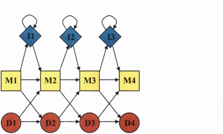
1.2 The match, delete and insert states of a profile hidden Markov model 24
1.3 Schematic diagram of the superfamily and sequence family levels in
the CATH d a ta b a s e ... 37
2.1 The common fold of ClpP protease and enoyl-CoA h y d ra ta s e ...40
2.2 Flowchart of the methods and data required for creating and main taining the D H S ... 46
2.3 Structural features of aspartate aminotransferase (PDB entry 2cst) . 48 2.4 Schematic TOPS diagram for the large domain of aspartate amino transferase ...49
2.5 LIGPLOT diagram for aspartate aminotransferase and the PLP co factor ... 50
2.6 Structural relationships between four members of the aspartate aminotransferase superfamily ... 51
2.7 DHS screen snapshot: Protein d e sc rip tio n s... 52
2.8 DHS screen snapshot: Enzyme classification n u m b e r s ... 53
2.9 DHS screen snapshot: SWISS-PROT d e s c rip tio n s ... 53
2.10 DHS screen snapshot: PROSITE p a t t e r n s ... 54
2.11 The CORA multiple structural alignment for the aspartate amino transferase su p erfa m ily ... 54
2.12 DHS screen snapshot: Ligand d a t a ...55
2.13 RASMOL superposition for four members of the aspartate amino transferase su p erfa m ily ... 55
2.14 DOMPLOT diagram for four members of the aspartate aminotrans ferase superfam ily...56
2.15 Sequence-structure plot for proteins within the aspartate aminotrans ferase superfam ily...57
2.16 Sequence identity distributions for proteins in four CATH superfolds . 58
List o f Figures 12
2.17 Pie chart showing the CATH classification methods used for 2,646
protein d o m a in s ... 61
3.1 Overview fiowchart of CATH sequence family g e n e r a tio n ...68
3.2 Principles of the DomainFinder a l g o r i t h m ...70
3.3 Schematic diagram of two multi-domain proteins th a t contain a com mon d o m a in ...72
3.4 Overview flowchart of the SPARTACLUS p ro to c o l...73
3.5 Coarse clustering of sequences using pairwise sequence identity . . . . 74
3.6 The programs within the HMMer software p a c k a g e ... 76
3.7 Refined clustering of sequences using iterated profile a n a ly s is ... 77
3.8 The SPARTACLUS protocol: An example s u p e r f a m ily ...78
3.9 Analysis of sequence clusters for profile d r i f t ... 80
3.10 Annotated tree diagram for the acid protease su p erfam ily ... 89
3.11 Manual analysis and definition of sequence cluster relationships . . . 90
3.12 Determining E-value parameters for SPARTACLUS refined clustering 91 3.13 Measuring the cluster ratio between CATH clusters and Pfam families 96 3.14 Histogram plot of the cluster ratio relationship between CATH clus ters and Pfam f a m ilie s ... 97
3.15 Measuring the cluster overlap between CATH clusters and Pfam families 99 3.16 Histogram plots of the cluster overlap relationship between CATH clusters and Pfam f a m ilie s ...100
3.17 Molscript pictures of proteins in the helix-hairpin-helix DNA repair enzyme su p erfam ily ...105
3.18 Annotated tree diagram for CATH superfamily 1.10.340.10 ... 107
3.19 Principal component analysis plot for CATH superfamily 1.10.340.10. 108 3.20 Molscript pictures of proteins in the legume lectin-like superfamily . . 109
3.21 Annotated tree diagram for CATH superfamily 2.60.120.60 ... I l l 3.22 Principal component analysis plot for CATH superfamily 2.60.120.60. 112 3.23 Molscript pictures of proteins in the aldolase s u p e rfa m ily ...113
3.24 Annotated tree diagram for CATH superfamily 3.20.20.70 ... 116
3.25 Principal component analysis plot for CATH superfamily 3.20.20.70. . 117
3.26 Schematic diagram of cross matches within CATH superfamilies . . . 120
3.27 Matrix of cross matches between refined clusters in the same super family...121
List o f Figures 13
3.29 Matrix of cross matches between refined clusters in different super
families... 124
3.30 World Wide Web interface to the CATH-PFDB HMM profile library 125
3.31 Graphical search results for scanning the sequence of human topoiso-
merase I against the CATH-PFDB HMM lib ra ry ...126
3.32 Molscript and DOM PLOT diagrams for human DNA topoisomerase I 127
4.1 Flowchart describing the generation of the benchmark test set of re
mote h o m o lo g u e s...137
4.2 Graphical description of the HSSP/Rost e q u a t i o n ... 139
4.3 The number of sequence matches associated with a range of Rost
th re s h o ld s ...140 4.4 Plot of sequence identity against alignment length for TESTSET816
false m a t c h e s ... 141
4.5 Plot of sequence identity against alignment length for TESTSET816
true m atch es...141 4.6 Overview of static profile library generation ... 144
4.7 Overview of the SAM-T99 protocol for detecting remote homologues . 145 4.8 Overview of dynamic profile library g e n e ra tio n ...146
4.9 Different approaches for calculating true and false positives for pair
wise and profile library s e a rc h e s 148
4.10 Basic file format for a ranked pair file ( R P F ) ... 150 4.11 Stages required to convert sequence search results into coverage-
versus-error p l o t s ...151
153 154
155
156
157
159 4.12 Coverage plots for different pairwise sequence search methods (I)
4.13 Coverage plots for different pairwise sequence search methods (II)
4.14 Coverage plots for SSEARCH using different sequence libraries .
4.15 Coverage plots for IMPALA using different substitution matrices
4.16 Coverage plots for different static profile library search methods
4.17 Coverage plots for different implementations of SAM software .
4.18 Match quality histogram plots for SSEARCH, HMMer-Local and
H M M e r-G lo b a l... 162
4.19 Match quality histogram plots for IMPALA, SAM-PFDB-CLW and
S A M -T 99-N R D B ...163
4.20 Schematic representation of sequence space for pairwise and profile
m e th o d s ...166
List o f Figures 14
5.2 Distribution of global RMSD values for the CASP3 ab initio structure
prediction c a te g o r y ...173
5.3 Examples of predictions for the m ainly-^ double sandwich cyanovirin (target 5 2 ) ...174
5.4 The SSAP residue environment scoring sch em e... 176
5.5 The SSAP histogram p l o t ...177
5.6 The SSAP coverage p l o t ...178
5.7 Lesk window plots ...179
5.8 Molscript diagrams for the top five predictions for target 77 ... 181
5.9 Secondary structure plots for the top five predictions for target 77 . . 182
5.10 SSAP histogram plots and Lesk window plots for target 7 7 ... 183
5.11 SSAP coverage plot for target 77 ...185
5.12 Molscript diagrams for the top five predictions for target 61 186
5.13 Secondary structure plots for the top five predictions for target 61 . .1 8 7 5.14 SSAP histogram plots and Lesk window plots for target 6 1 ... 188
5.15 SSAP coverage plot for target 61 189
List o f Tables
1.1 Location of the principal DNA sequence d a ta b a s e s ... 18
2.1 The number of branches at each hierarchical level in the CATH
database (release 1 .7 ) ... 42
2.2 World Wide Web resources used by the Dictionary of Homologous
S u p e rfa m ilie s... 45
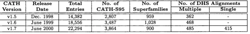
2.3 The number of DHS alignments for each CATH database release . . . 47
2.4 Description of the four sequence families in the aspartate aminotrans
ferase superfam ily...51
2.5 Statistics for four superfolds in the CATH d a t a b a s e ...59
3.1 The number of genomic sequence regions corresponding with CATH
structural domains ( v l.6 .2 )... 71 3.2 Glossary of abbreviated terms used in this c h a p te r ... 75
3.3 Structural and functional descriptions of the CATH-PFDB 52 super
family test s e t ... 84
3.4 Coarse and refined clustering statistics for the 52 superfamily test set 93
3.5 Iteration statistics for the CATH-PFDB 52 superfamily test set . . . 94
3.6 Summary of the overall match between CATH refined clusters and
Pfam families in the tRNA synthetase (class II) s u p e r f a m ily ... 101
3.7 Cluster overlap details for 19 Pfam families with multiple CATH clusters 102
3.8 Cluster overlap details for 15 Pfam families with multiple CATH clusters 103
3.9 Summary of the three CATH superfamilies selected to describe the
SPARTACLUS protocol ...104
3.10 Summary of sequence cluster properties for CATH superfamily
1.10.340.10 ... 106
3.11 Summary of the overall match between CATH refined clusters and
Pfam family definitions for superfamily 1.10.340.10... 107
3.12 Summary of sequence cluster properties for CATH superfamily
2.60.120.60 110
List o f Tables 16
3.13 Summary of the overall match between CATH refined clusters and
Pfam family definitions for superfamily 2.60.120.60... I l l
3.14 Summary of sequence cluster properties for CATH superfamily
3.20.20.70 ... 115
3.15 Summary of the overall match between CATH refined clusters and
Pfam family definitions for superfamily 3.20.20.70... 116
3.16 Refined clustering statistics for the whole CATH-PFDB database . . 118
3.17 Cross matches between refined clusters in the same superfamily. . . .121
3.18 Cross matches between refined clusters in different superfamilies. . . .1 2 3
3.19 Tabular search results for scanning the sequence of human topoiso
merase I against the CATH-PFDB HMM lib ra ry ...126
4.1 The number of different structural classification levels in the
RE-MOTE303 test set ...140
4.2 Pairwise search algorithms and p a ra m e te rs ... 142 4.3 Profile search algorithms and p a r a m e te rs ... 144
4.4 Description of four different profile library approaches th a t use SAM
s o f tw a r e ... 146
4.5 Definitions used for measuring the performance of sequence search
a lg o rith m s...147
4.6 Relationship between observed errors and E-value for SSEARCH and
the REMOTE303 benchmark sequences... 149
4.7 Summary of the coverage results for different pairwise methods . . . .1 5 3
4.8 Summary of the coverage results for SSEARCH using different se
quence l ib r a r ie s 155
4.9 Summary of the coverage results for IMPALA using different matrices 156 4.10 Summary of the coverage results for static profile m e t h o d s ... 157
4.11 Summary of the coverage results for different implementations of SAM
s o f tw a r e ... 159 4.12 Summary of the quality of the REMOTE303 sequence matches . . . . 160
4.13 Summary of benchmarking c o n c lu sio n s ...168
5.1 Descriptions of the fifteen ab initio t a r g e t s ... 172 5.2 The top five predictions for target 77 ranked by SSAP criteria . . . . 184
5.3 The top five predictions for target 61 ranked by SSAP criteria . . . . 187 5.4 The top five prediction groups for the medium and hard targets . . . 190
5.5 A short description of the structure prediction methods used by
C hapter 1
In trod u ction
1.1
P r o te in s
Proteins play key roles in virtually all biological processes (Stryer, 1995). They
mediate a remarkably diverse range of functions including catalysis, transport and
storage, mechanical support, co-ordinated motion, immune protection and the con trol of growth and differentiation. In 1951, Sanger and Tuppy demonstrated the
linearity of proteins through sequencing a single chain of the polypeptide hormone insulin (Sanger & Tuppy, 1951). Sequencing was initially carried out on polypep
tides due to their stability and relative ease of purification. The main technique used
was the manual process of sequential Edman degradation (Edman, 1950). It was not
until the techniques of gene cloning and PCR (Polymerase Chain Reaction) provided
large amounts of purified DNA did the focus turn to nucleic acid sequencing. In 1975, Sanger and Coulson developed a rapid method for determining nucleotide sequences
(Sanger & Coulson, 1975). This method and subsequent improvements (Wu, 1978)
coupled with the continued development in autom ated techniques has facilitated the
rapid growth in sequencing to the point where we now have a rough draft of the
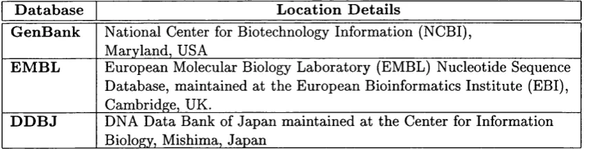
human genome (Lander et ai, 2001). The DNA sequences are stored at three major
DNA sequence databases, GenBank (Benson et ai, 2000), EMBL (Stoesser et a/.,
2001) and DDBJ (Tateno et ai, 2000). The location of these databases is shown in
table 1.1. The GenBank database contained 12,244,000 nucleotide sequence records
as of June 2001 (data from http://w w w .ncbi.nlm .nih.gov/G enBank).
Chapter 1. Introduction 18
D a ta b a s e L o c a tio n D e ta ils
G e n B a n k N ational Center for Biotechnology Inform ation (NCBI), M aryland, USA
E M B L European Molecular Biology L aboratory (EMBL) Nucleotide Sequence Database, m aintained at the European Bioinformatics Institute (EBI), Cambridge, UK.
D D B J DNA D ata Bank of Jap an m aintained a t the Center for Information Biology, Mishima, Japan
T a b le 1.1: Location of the principal DNA sequence databases.
1.1.1
P rotein Sequence D atab ases
A considerable amount of the information in the nucleic acid sequence databases
comes from non-expressed DNA sequences (promoter regions, binding sites etc.).
However, a large proportion represent genes or Open Reading Frames (ORFs) th a t can be translated to yield a protein product. Simple genomes, such as those from
prokaryotic organisms, contain genes whose linear structure is directly related to the
translated product. In eukaryotic organisms, the genes contain both translated (ex
ons) and untranslated (introns) regions. This complicates the process of identifying the protein product.
1.1.1.1 P I R /P S D
The Protein Sequence Database (PSD) was the first collection of sequences to be established. It was developed by M argaret Dayhoff in the 1960’s and is currently
maintained as the Protein Information Resource (PIR) International PSD (Barker
et al., 2001). This is a world wide consortium th a t includes the Protein Information Resource, the Protein Information Database of Japan (JIPID) and the Martinsried
Institute for Protein Sequences (MIPS). The PIR is divided into four sections, P IR l
to PIR4, th at differ in terms of the quality of d a ta and annotation provided. The
latest release of the P IR /PSD database (version 69.01) contained 237,651 entries
(data from http://pir.georgetow n.edu).
1.1.1.2 S W IS S -P R O T
SWISS-PROT (Bairoch & Apweiler, 2000) is a manually maintained sequence
database th at endeavours to provide high-level annotations, including descrip
tions of protein function, post-translational modifications and domain structure.
SWISS-PROT entries also contain cross-references to bibliographic references, pro tein family databases and functional or disease state resources. The most recent
Chapter 1. Introduction 19
http://w w w .expasy.org/sprot). SWISS-PROT is supplemented by a computer anno
tated database called TrEMBL (Translation of EMBL nucleotide sequence database,
Bairoch & Apweiler, 2000). TrEMBL is based on the translation of coding sequences
from the EMBL database. The resource exists to store the ever-increasing number of
protein sequences obtained from genome sequencing projects without compromising
the quality of the SWISS-PROT database. Release 17.3 of the TrEMBL database
contained 471,191 entries.
1.1.1.3 N R D B
The NRDB (Non-redundant Database) is a composite of GenPept (automatic
translations from GenBank), SWISS-PROT, PIR and PDB sequences (Benson
et ai, 2000). The database is comprehensive and up-to-date but is actually non identical rather than non-redundant, with only identical sequences removed from
the database.
1.2
P r o te in S eq u en ce C o m p a riso n
1.2.1
Sequence Sim ilarity
The relationship between two proteins th a t have descended with divergence from a
common ancestor is defined as homologous (Fitch, 1970). It is useful to distinguish between two types of homologues. Proteins th at have evolved from a common
ancestral gene by spéciation and perform the same or similar function in different
species are called orthologues. Paralogous proteins arise from the duplication of a
single gene and exist within the same organism. They can evolve new functions once
free from the constraints of natural selection (Henikoff et al, 1997).
The central hypothesis of sequence analysis is th at sequence similarity can be
used to identify homologous relationships. Sequence similarity can be measured in
terms of the number of identical residues shared between two proteins. This is often expressed as a percentage of the length of the smaller protein (percentage identity).
High identity can be used to indicate homology (Ghothia & Lesk, 1986; Hubbard &
Blundell, 1987; Sander & Schneider, 1991; Flores et al, 1993). However, it becomes
difficult to assign relationships when the level of identity falls below 30% into the
region known as the ‘twilight zone’ (Doolittle, 1986). To measure similarity, the sequences must first be aligned to take into account the insertions and deletions
(indels) th at have occurred over the course of evolution. This process introduces
Chapter 1. Introduction 20
Small
P rolin e
T iny
A liphatic
C harg ed N eg ativ e '
Polar
A rom atic
P o s itiv e
Hydrophobic
F i g u r e 1 .1 : Venn diagram of th e chem ical and physical p ro p erties of am ino acids (Taylor, 1986a). T h e am ino acids are alanine (A), cysteine (C ), asp a rtic acid (D), glutam ic acid (E), phenylalanine (F), glycine (G ), h istidine (H), isoleucine (I), lysine (K ), leucine (L), m ethionine (M ), asparagine (N), proline (P ), g lutam ine (Q ), arginine (R ), serine(S), threonine (T ), valine (V), try p to p h a n (W ) and tyrosine (Y).
into register. Alignm ent of the secpiences highlights positions t h a t are conserved and also those t h a t have changed over time.
1.2.1.1 P h y sic o c h e m ic a l P r o p e r tie s o f A m in o A cids
Proteins are composed of am ino acids of which there are 20 n a tu ra lly occurring variations. A lthough each am ino acid has a distinct chemical structure, they can be grouped together on the basis of their chemical an d physical properties. This can be visualised as a Venn diagram (Taylor, 1986a) as shown in figure 1.1.
Chapter 1. Introduction 21
1.2.1.2 T he M u ta tio n D a ta M atrix (M D M )
The M utation D ata M atrix (MDM) was developed by Dayhoff and is derived from
the comparison of closely related sequences i.e. >85% sequence identity (Dayhoff,
1978). The matrices are based on the concept of the Point Accepted M utation
(PAM). The probability of a residue m utating during an evolutionary distance in
which one point m utation occurs per 100 residues corresponds with a distance of
1 PAM. Matrices corresponding with larger evolutionary distances are obtained by
multiplying the original m atrix by itself, for example, the PAM 250 m atrix reflects
sequence identity levels of 20% between two proteins.
1.2.1.3 T h e B lock s S u b stitu tio n M atrices (B L O SU M )
The BLOSUM series of matrices (Henikoff & Henikoff, 1992) are generated from con
served blocks of aligned sequences th at comprise the BLOCKS database (Henikoff & Henikoff, 1991). The blocks can contain sequences from a wide range of evolution
ary distances. In order to produce matrices th a t reflect substitutions from a defined evolutionary distance, the sequences within the blocks must be clustered. This pro
cess requires calculating the pairwise sequence identity for every pair of sequences. The sequences are then clustered for a given identity threshold according to the
rule th a t any pair of sequences th at have a percentage identity above the threshold
are merged together. In calculating the observed substitutions within each block,
the contributions from within a cluster are averaged. For example, the BLOSUM50
m atrix uses a clustering threshold of 50% identity. A series of BLOSUM matrices at different clustering thresholds have been created and shown to outperform the
PAM matrices in searching for a defined set of homologous relationships (Henikoff
&: Henikoff, 1993).
1.2.2
Pairw ise Sequence A lignm ent
1.2.2.1 R igorous A lign m en t A lgorith m s
Needleman & Wunsch (1970) were the first to propose a dynamic programming
algorithm for the comparison of macromolecular (protein or DNA) sequences. Dy
namic programming enables the optimal alignment to be found efficiently without
checking all possible alignments. The Needleman and Wunsch algorithm performs a
‘global’ alignment of two sequences i.e. all sequence positions are taken into account
Chapter 1. Introduction 22
two sequences, it is useful to consider the local alignment between a substring of
each sequence. Smith and W aterman introduced a minor modification to the global
dynamic programming algorithm to enable optimal ‘local’ alignments between two
sequences to be identified (Smith & W aterman, 1981).
1.2.2.2 H eu ristic A lgorith m s for Sequence A lig n m en t
Several heuristic algorithms have been developed to speed up the alignment proce
dure. The two main algorithms are FASTA (Pearson & Lipman, 1988) and BLAST
(Altschul et al, 1990, 1997), although they are not guaranteed to find the optimal
alignment, they make it practical to undertake routine large scale sequence database
searching. FASTA creates a hash table of all k-tuples (a string length of k) in the
query sequence and uses this to efficiently find identities between the query sequence and the database sequences. For protein sequences, k-tuple values of 1 or 2 are used
with 1 giving higher sensitivity. The identified regions can then be optimally aligned
using dynamic programming. BLAST also uses a word-based heuristic to approx imate a simplified Smith-W aterman algorithm called the Maximal Segment Pairs
algorithm. Tripeptide words (strings of 3 residues) from the query sequence are ‘ex panded’ to include all tripeptides th at score above a threshold when aligned to the
initial tripeptide using a substitution m atrix e.g. BLOSUM62. Tripeptide identities
between query and database sequences from the expanded list are quickly identi
fied and combined to give ungapped High Scoring Segment Pairs (HSPs). Gapped
alignments are created by using the Smith-W aterman algorithm to extend matches in both directions of the alignment.
1.2.2.3 Scoring th e A lign m en t
Once two sequences have been aligned, it is necessary to consider whether the rela
tionship has occurred as a result of evolution (i.e. descent from a common ancestor)
or has arisen by chance. Statistical theories have been developed to convert align
ment scores into probability values to answer this question (Karlin & Altschul, 1990;
Altschul et ai, 1994; Dembo et al, 1994; Altschul & Gish, 1996). These are based on
the observation th a t the distribution of alignment scores for comparisons between
random sequences can be approximated by the Extreme Value Distribution (EVD,
Dembo et al, 1994). For database searching, it is common to use the expectation
value (E-value) as a measure of statistical significance. For a given alignment with
score S, the E-value is defined as the expected number of distinct sequence matches
Chapter 1. Introduction 23
D sequences. For example, an E-value of 1 assigned to a sequence match indicates
th a t one match of equal or better score would be expected by chance alone in the
current search. An E-value of zero corresponds with no expected chance matches.
1.2.3
Profile-based Sequence C om parison A pproaches
Pairwise sequence comparison techniques such as BLAST and FASTA generally as
sume th a t all amino acid positions are equally im portant. However, a multiple align
ment of a protein sequence family can highlight residues th a t are more conserved
than others (e.g. in the active site) or positions where insertions and deletions are more frequent (e.g. loop regions). Several sequence ‘profile’ methods were developed
in the 1980’s (Taylor, 1986b; Gribskov et a/., 1987; Barton k, Sternberg, 1990) to
capture this position-specific information. Formally, a sequence profile is defined as
a consensus prim ary structure model consisting of position-specific residue scores and insertion or deletion penalties (Eddy, 1996). In the classical profile method of
Gribskov et al. (1987), the amino acid substitution scores are created by summing
Dayhoff exchange m atrix values (Dayhoff, 1978) according to the observed amino acids in each column of the alignment. Gap penalties are reduced at alignment posi
tions with gaps, according to the length of the longest insertion spanning th a t point
in the alignment. A modified Smith-W aterman dynamic programming algorithm is used to align the sequence to the profile.
1.2.3.1 H id d en M arkov M od els
The underlying model represented by a profile closely resembles the hidden Markov
models (HMMs) introduced for describing protein families (Krogh et 1994; Baldi
et al, 1994). An HMM is a mathem atical model which produces a stream of ob servable information in a probabilistic manner. HMMs are a general statistical
modelling technique particularly suited to ‘linear’ problems, and have been widely
used in speech recognition for many years (as reviewed by Rabiner, 1989). In the
case of protein sequences the observable information is in the form of amino acids,
and the HMM can be considered to be a sequence generating factory capable of
producing many different sequences with different probabilities.
More specifically, an HMM is a series o f ‘states’ interconnected by state-transition
probabilities. In the profile HMM architecture introduced by Krogh et al. (1994)
and modified by Eddy (1998), each conserved column in a multiple alignment is
Chapter 1. Introduction 24
M3
M4
M l
M2
M D3
D1
F ig u r e 1.2: T he profile hidden Markov model is characterised its m atch (M ), delete (D) and in sert (I) states and the allowed tran sitio n s (arrow s) betw een them .
110 am ino acid present at this position and an insert s ta te allows for the insertion of
one or more am ino acids after the m atch position. S ta r tin g from an initial state, a secpience of states is generated by moving from s tate to s ta te according to the state- transition probabilities until an end s ta te is reached. Each s ta te ‘e m its ’ symbols (residues) according to its emission probability d istribution, creating an observable sequence of symbols (Eddy, 1996). The sequence of states is a first-order Markov chain as the choice of the next sta te to occupy is depen d e n t on the identity of the current state. However, the s tate sequence is not observed, it is hidden, only the symbol sequence is observed and the most likely s ta te sequence must be inferred from an alignm ent of the HMM to the observed sequence (Eddy, 1996).
Two popular HMM software packages are SAM-T99, a development of the SAM- T98 protocol (K arpins et al., 1998) and the unpublished H M M er software (reviewed in E d d y (1998)). SAM-T99 is a tool for detecting rem ote homologues, typically ini tia te d from a single sequence. The HMMer package requires pre-generated multiple alignm ents in order to build HMMs and is used to search and m ain tain the Pfam d a ta b a s e (B atem an et a i , 2000).
1.2.3.2 P S I-B L A S T
Chapter 1. Introduction 25
ate a multiple alignment from which a profile is estimated. In the second iteration,
the profile is used to search the database and the process is repeated until no more
homologues are found or a set number of iterations are reached. A key develop
ment for detecting genuine homologous relationships has been the availability of
robust statistical estimates. This enables the autom atic execution of iterative pro
file searches.
Sequence searching methods th a t use profile-based approaches or intermediate
sequences e.g. PSI-BLAST, hidden Markov models (SAM-T98), IBS (Park et al.,
1997) and MISS (Salamov et al., 1999a) have been shown to detect more distant
homologues than pairwise sequence techniques (Park et al., 1998; Salamov et al.,
1999a). Other sequence searching methods include GeneQuest (Taylor, 1998; Taylor
& Brown, 1999) and BASIC (Rychlewski et al, 2000).
1.2.4 M u ltip le Sequence A lignm ent
Optim al multiple sequence alignment methods are too computationally expensive to
be used for aligning large numbers of sequences. Therefore, the heuristic approach adopted by progressive alignment methods is the most commonly used multiple
alignment method. Progressive alignment consists of three steps th a t can be done separately or merged together. The first stage involves computing the alignment
scores for all pairs of sequences. This information is then used to build a guide
tree to reflect the similarities between the sequences. The sequences are aligned according to the order of the tree with the most similar sequences aligned first.
The algorithm aligns the two sequences or alignments th a t are associated with the
two daughter nodes of each node of the tree. ClustalW, one of the most popular
alignment packages, uses the Neighbour-Joining algorithm (Saitou & Nei, 1987) to
construct the guide tree and profile alignment with position-specific gap penalties to
align two alignments (Thompson et al, 1994, 1997). Progressive alignment speeds
up the alignment process at the cost of fixing alignments at an early stage of de
velopment. Other approaches are now incorporating predicted secondary structure
and re-evaluating the alignments at later stages in the process (Heringa, 1999).
1.3
P r o te in F am ily D a ta b a se s
Sequence families represent collections of homologous proteins th a t share a com mon ancestor. Bringing together related proteins in a multiple sequence alignment
Chapter 1. Introduction 26
structure and function of the proteins in the family are less tolerant to m utation
and are therefore more conserved. Homologous relationships can be identified rela
tively easily if the divergent proteins retain high sequence identities of 30% or more
(Chothia & Lesk, 1986; Sander & Schneider, 1991; Rost, 1999). The presence of a
functional sequence motif (PROSITE) or set of motifs (PRINTS) can be used to de
tect more distant sequence relationships. These are described in more detail below.
Over long periods of evolution, all traces of sequence similarity between two related
proteins can disappear. In these situations, structural similarity (if available) can
provide the evidence th a t the proteins are homologous as structure is typically more
conserved than sequence (Chothia & Lesk, 1986; Flores et al, 1993).
1.3.1
M anually C urated D atab ases
Protein family databases are now well-established tools for protein sequence analysis.
They include the widely used resources, PROSITE, BLOCKS, Pfam and PRINTS. Searching a protein family database can be more sensitive and produce a more
concise list of matches than a primary sequence databank search.
1.3.1.1 P R O S IT E
The PROSITE database contains both regular expression-like patterns and profiles
to describe sequence families (Hofmann et al, 1999). The patterns are typically
chosen to encapsulate biologically significant regions of sequence th a t can be used to
characterise the function of the proteins in the family. PROSITE provides extensive
documentation in the form of a concise description of the protein family or domain
and a summary of the reasons for the development of the pattern or profile. Release
16.43 of PROSITE (August 2001) contained 1,090 documented entries describing 1,476 different patterns and profiles.
1.3.1.2 P R IN T S
PRINTS is a database of protein family ‘fingerprints’, a series of un-weighted se
quence motifs th a t characterise an aligned family (Attwood et al, 2000). Instead
of the binary ‘hit-or-miss’ approach of regular expression pattern matching, finger
prints are able to tolerate mismatches at the level of residues within individual motifs
and at the level of motifs within fingerprints. The resource can be searched using
pattern or profile methods (Scordis et al, 1999) and also using BLAST (Wright
Chapter 1. Introduction 27
were 1,550 entries in the PRINTS database (release 31.0, June 2001) corresponding
with 9,531 sequence motifs.
1.3.1.3 BL O C K S
The BLOCKS database uses multiple ungapped local alignments, called blocks, to
describe family membership (Henikoff & Henikoff, 1991). The blocks are created
using an autom ated method called PROTOMAT th at detects the most highly con
served regions of each protein family (Henikoff et ai, 1995). The raw sequences
of each block are stored in the database. In addition, the sequences in each block
are assigned sequence weights to represent their divergence from other members.
This weighting is taken into account for scoring a sequence match to a sequence in a block. The BLOCKS-f- resource is a recent addition to the BLOCKS database
(Henikoff et ai, 1999). The protein family coverage has been increased by calcu
lating blocks from other databases such as ProDom (Corpet et al, 2000), PRINTS
(Attwood et ai, 2000), Pfam (Bateman et ai, 2000) and DOMO (Gracy & Argos,
1998). Version 13.0 of the BLOCKS Database consisted of 8,656 blocks representing
2,101 families.
1.3.1.4 P fam
Pfam is a large collection of multiple sequence alignments and profile hidden Markov
models (HMMs) for protein domain families (Bateman et u/., 2000). Seed alignments
for each family are manually constructed and HMMs are used to automatically
identify members of the family outside the seed sequences. In addition to the curated
families, called Pfam-A, a supplementary resource, Pfam-B, has been created based
on the automatically generated families of ProDom (Corpet et ai, 2000) to provide
completeness in terms of sequence coverage. Version 6.6 of the Pfam database
August 2001) contained 3,071 Pfam-A families (267,598 sequences) and 57,477 Pfam-
B families (126,378 sequences).
1.3.1.5 InterP ro
InterPro is an integrated document resource for protein families, domains and
functional sites (Apweiler et a/., 2001). It combines the efforts of the PROSITE,
PRINTS, Pfam and ProDom database projects into a single coherent resource. The
member databases will continue to exist separately and co-ordinate their selection
of families to document in an attem pt to minimise any duplication of effort in the
Chapter 1. Introduction 28
1.3.2 A u tom atically C lustered Sequence D atab ases
Unlike signature databases, clustered resources are derived autom atically from the
primary sequence databases using different clustering algorithms. The usual clus
tering strategy is to perform a database search with BLAST or FASTA, followed
by grouping sequences together based on the statistical scores. For example, in
the SYSTERS protein sequence cluster protocol (Krause et ai, 2000), single link
age clustering is applied using BLAST E-values. Clusters are created at different
E-value thresholds to generate a hierarchy of families called the SYSTERS tree.
Problems can arise due to the multi-domain nature of proteins. As a result several
autom atic domain detection algorithms have been developed such as DOMAINER
(Sonnhammer & Kahn, 1994), MKDOM (Gouzy et ai, 1999) or DIVCLUS (Park &
Teichmann, 1998). Recently, May (2001) suggested the use of sequence weighting
and dynamic programming to optimally classify proteins without using subjective
thresholds to define group membership.
1.4
P r o te in S tr u c tu r e
At the atomic level, the structure of a protein determines its function. Detailed
three-dimensional structures reveal mechanistic aspects of a proteins function th at are critical for understanding biological processes. As proteins diverge during the
course of evolution, their structures change to accommodate the differences in amino
acid size and polarity caused by mutations. The structural core often remains very
similar with insertions or deletions occurring in loop regions th a t connect the sec
ondary structure elements (SSEs) (Chothia & Lesk, 1986). In some cases, supersec ondary motifs or small domains are inserted into these loops. Insertions are rarely
seen within SSEs (Pascarella & Argos, 1992), however the m utation of core residues
can cause significant changes to the orientations of the SSEs.
Since the preliminary structure of myoglobin was determined by Kendrew and
co-workers (Kendrew et ai, 1958) the field of structural biology has grown tremen
dously. The Protein D ata Bank (PDB) now contains the co-ordinates of more than
14,000 protein chains consisting of over 27,000 structural domains determined by X-
ray crystallography or NMR (Abola et al., 1987; Berman et ai, 2000). Almost 3,000
new structures were deposited last year (2000) and this number is set to increase as
structural genomic projects gather momentum (Pennisi, 1998). It becomes increas
ingly im portant th at this structural data is organised and annotated in a biologically
Chapter 1. Introduction 29
1.4.1 Structure C om parison M eth od s
1.4.1.1 R igid B o d y S u p erp osition
The first structure comparison techniques used a rigid-body superposition of equiv
alent residues (Rossmann & Argos, 1975). This leads to the calculation of the root
mean squared deviations (RMSD) over all atoms th a t represents the average distance
between the two proteins. However, structural embellishments can significantly af
fect this value. This has lead to calculating RMSD over equivalent residue pairs
within a certain distance threshold from each other. This has been shown to be a
better indicator of structural similarity than global RMSD (Chothia & Lesk, 1986;
Wilson et ai, 2000). There are now many structural comparison methods th a t have
been developed (see Holm & Sander (1994b), Orengo (1994) and Brown et al. (1996)
for reviews). The algorithms fall into two main categories, those th at attem pt to
superpose structures by minimising the inter-molecular distance between equivalent positions, and those th at compare intra-molecular distances between residues or sec
ondary structures. Dynamic programming, used for sequence comparison to handle
insertions and deletions, has also been applied to structural comparison methods.
1.4.1.2 SSA P: Sequential S tructural A lig n m en t P rogram
The SSAP method is a distance plot-based approach for structural comparison
(Taylor & Orengo, 1989; Orengo et ai, 1992). Distance or contact plots are two-
dimensional matrices, labelled horizontally and vertically with the protein’s sequence
and shaded according to whether pairs of residues are in contact in the structure
(Phillips, 1970). In the SSAP method, the three-dimensional internal geometry between proteins is compared using the Needleman-Wunsch algorithm to identify
equivalent positions. The structural environment or view for each residue is de
scribed by the set of vectors from the Cp atom to the Cp atoms of all other residues.
The common frame of reference for each residue view is based on the tetrahedral
geometry of the Cq atom. Dynamic programming is first applied to compare residue
views for each pair of residues between the two structures. The optimal alignment
path through each residue view m atrix is added to a summary m atrix and dynamic
programming is used again to determine the final alignment of residues. This use
of dynamic programming on two levels has been described as double dynamic pro
gramming. The scoring scheme is normalised to return a score between 0 and 100,
with 100 being a perfect match. SSAP scores above 80 are associated with highly
similar structures, suggesting they are descended from a common ancestor (Orengo
Chapter 1. Introduction 30
the evolutionary relationship between the two proteins can still be unclear without
supporting functional evidence.
1.4.1.3 O ther S tru ctu re C om parison M eth o d s
The DALI method (Holm & Sander, 1993) uses simulated annealing to build an
alignment of equivalent hexapeptide backbone fragments between two proteins. The
two stage process first compares hexapeptide contact maps (built using atoms)
to establish equivalent fragments. In stage two, different hexapeptide fragments are combined using simulated annealing. The advantage of this approach is th at
the alignment is not built in a structurally sequential manner allowing comparisons
between topologically different proteins to be performed (Brown et ai, 1996). DALI
is the structure comparison method used to construct the Dali Domain Database
(Holm & Sander, 1999).
Structural comparison is typically much slower than sequence comparison, there
fore approaches to speed up the process have been investigated. Alternative al
gorithms such as geometric hashing or graph theory have been implemented in addition to using simplified representations of protein structure For example, the
VAST structure comparison algorithm (Madej et a/., 1995) used within the MMDB
(Marchler-Bauer et ai, 1999) uses graph theory to rapidly m atch secondary struc
ture elements. Both DALI and VAST use statistical measures such as Z-scores to
provide an estimate of the significance of the structural match in relation to the
background distribution of scores.
1.5
P r o te in S tr u c tu r e C la ssifica tio n
1.5.1 Structural C lassification D atab ases
Protein structure classification databases, CATH (Orengo et al, 1997), SCOP
(Murzin et al, 1995), Dali Domain Dictionary (Holm & Sander, 1999), 3Dee (Sid-
diqui et al, 2001), DDBASE (Sowdhamini et al, 1996) and ENTREZ/M MDB
(Hogue et al, 1996; Marchler-Bauer et al, 1999) are now well established and pro
vide frameworks for ordering the known protein universe. These databases cluster
proteins on the basis of both geometrical and evolutionary considerations. The
approaches vary from manual methods (Murzin et al, 1995) to the application of
autom atic structure comparison methods i.e. SSAP (Taylor & Orengo, 1989), DALI (Holm & Sander, 1993), STAMP (Russell & Barton, 1992), DIAL (Sowdhamini &
Chapter 1. Introduction 31
for structural similarity and groups apply different criteria for assigning proteins to
fold groups.
CATH and SCOP are currently the largest manually validated hierarchical clas
sifications of protein domain structures (Pearl et al, 2001b; Lo Conte et ai, 2000).
Both these databases group proteins into homologous families and superfamilies. Homologous families contain proteins th at have descended from a common evolu
tionary ancestor and share similar functional properties, although the proteins may
not have significant sequence identity. The structural superfamily level clusters to gether protein families th a t often have different functions but they can be shown
to have evolved from a common evolutionary ancestor. This evidence is usually
derived from structural comparisons or the literature. Both these levels are interest
ing to many biologists as they cluster proteins whose core structural and functional
features have often been conserved by evolution (Chothia, 1984; Overington et al.,
1990). Identifying the homologous superfamily of a protein of interest can be an
im portant step in determining the biological role of the protein.
More recently, databases have emerged th at present structural alignments for se
lected protein families. HOMSTRAD (Mizuguchi et ai, 1998b) contains 585 align
ments for homologous families originally developed by Overington et al. (1990).
CAMPASS (Sowdhamini et al., 1998) is a database of 863 protein superfamilies de
rived from DDBASE. In both cases the alignments are annotated with structural
features using JOY (Mizuguchi et al., 1998a).
1.5.2
G eom etric C onsiderations
Proteins are assigned to a particular structural class on the basis of the secondary structure composition and packing (Levitt & Chothia, 1976). Class can be divided
into mainly-CK, mainly-^ and a{3. In some classifications, the class is divided into
a+/3 and alternating a//3 groupings. The a-i-p group involves the a and /3 units to
be segregated along the protein chain, while a//3 contains mixed or alternating a and
13 units. W ithin each class, proteins are clustered according to the spatial orientation
of the secondary structure elements and their connectivity. This is described as the
protein fold or topology. Different folds are considered to be those with different
connectivities between the secondary structures although the overall geometry may
be similar. Estimates of the number of folds observed in nature varies from hundreds
to several thousands (Orengo et al, 1994; Govindarajan et ai, 1999; Wolf et ai,
2000). These attem pts are hampered by two types of bias in the structural data.