Required Bandwidth Capacity Estimation
Scheme For Improved Internet Service Delivery:
A Machine Learning Approach
Mba. O. Odim, Victor C. Osamor
Abstract This paper proposed a data driven, machine learning traffic modelling approach for estimating required bandwidth during telecommunication
planning for good quality service delivery. The multilayer perceptron was employed to estimate the offered traffic, a safety factor was incorporated to ensure smooth flow of traffic and a neutralisation factor for moderating under or over provisioning of the bandwidth resource. The offered traffic input lags were varied from 1 to 24. The training epoch values of 200, 500, and 1000 on one and two hidden layered networks were used. The learning algorithm was backpropagation with 0.1 learning rate and 0.9 momentum on logistic sigmoid activation function. The scheme was implemented in Visual Basic and compared with four existing statistically based bandwidth estimation formulae, using four categories of classified traffic of a residential network of a firm in Nigeria. The findings revealed that the proposed scheme gave the minimum cost function, loss rate, and the highest average utilisation on two of the traffic categories (the HOURLY_IN and of HOURLY_OUT), outperformed two of the existing models on the DAILY_IN traffic category and one of the existing models on the DAILY_OUT traffic set. The study recommended that the proposed scheme would serve more effectively toward enhancing internet management related tasks such as general resource capacity planning.
Index Terms: Bandwidth Estimation; Internet Service; Machine learning; Traffic forecasting. Multilayer Perceptron, Safety margin, neutralization factor
————————————————————
1
INTRODUCTION
THE quality of an internet service depends largely on the availability and adequacy of some critical resources such as the bandwidth. Sufficient bandwidth is required to guarantee smooth flow of traffic, ensure correct performance of applications, and/or maintain a satisfactory quality of service [1]. Bandwidth Provisioning remains a critical issue of concern in Africa for effective internet connection and access. [2] attributed the inability of internet Service Providers in meeting the internet service delivery needs of users to insufficient and high cost of bandwidth. The study showed that the amount of bandwidth allocated to the Management Institute of Technology (MIT), Boston, USA was quite larger than all bandwidth allocated to Nigeria as a whole. It was further noted that insufficient bandwidth, had been a bottleneck to active research and development in Higher institutions of learning in Nigeria. A study conducted by [3] reported that bandwidth cost had been approximately ten times more in Africa than they were in North America and Europe, and that it could be up to hundred times more for broadband connection. This situation has not drastically improved. Bandwidth resource provisioning depends on accurate information about offered traffic [4] .Traffic means are used by operators to, roughly estimate bandwidth capacity. More precise estimates are based on traffic statistics obtained from packet captures, such as variance. To ensure smooth flow of traffic, provision needs to be made to cater for sudden burst [5].
A quick approach to ensure a resource does not constrain the smooth flow of traffic, is to increase the capacity of the resource. However, this approach may not be sustainable due to the fact that resource demand varies and the budget of resources is limited [6]. In addition, traffic data experience high degree of variability, at some point activities are low and at other time the activities are high. [7] observed that traditional bandwidth provisioning formula had been merely based on intelligent guesses. For instance, thirty percent added to the average traffic rate. However, such method neither guarantees no waste of resources nor availability of sufficient resources, resulting to under-forecasting on one hand and as well as over-forecasting on the other hand. Under over-forecasting leads to under-provisioning and this restrict resources and consequently lead to loss of information and poor QoS. Over forecasting on the other hand, leads to over-provisioning which results to wastage of resources and high operational cost. Analytical techniques based on statistical approaches have been applied to traffic modelling and resource estimations. However, the techniques are based on assumptions that are difficult to accurately model the high degree of variability and nonlinearity of Internet traffic, resulting to either high resource costs or constraining smooth flow of traffic. Traditional statistical methods have focused on situations in which data show low or moderate variability and high degree of linearity. Traditional statistical methods also commonly assume that measured data are approximately normally distributed. In contrast, internet measurements are often quite different. In most cases, internet traffic shows high degree of variability [8]. Machine learning techniques have shown strong capability for modelling nonlinear relations and high degree of data set. However, their applications have been mainly limited to traffic forecasting. In the light of the above discussion, this study, therefore proposed a cost-effective scheme for estimating required bandwidth for predicted offered internet traffic.
_____________________________
Mba O. Odim is a Senior lecturer in the Department of Computer Science, Redeemer’s University, Ede, Nigeria. E-mail: [email protected]
327
2 R
ELATEDW
ORKA number of studies have been reported as an attempt in addressing the deficiencies of the existing estimation approaches. [9] proposed an estimation approach that used average traffic rate and its variations at small timescales, with a desired level of performance based on stationarity of input traffic process for Gaussian distribution of traffic and general queuing model. The approach was validated in [10] and [7], where the estimation scheme was expressed as a function of the average traffic rate, traffic variance and the required performance level. In these approaches, precise estimate of the average traffic and the traffic variance were critical. It was rather hard to measure the traffic variance compared to the average traffic rate; due to the measurement on small timescales required. In [11], a bandwidth estimation approach that determines the lowest amount of bandwidth level for a network link that guarantees a level of performance as a function of a given traffic load was proposed. Packets captured from IP-based networks were used to validate the study. The findings from the study showed a higher precision values for the heavy tailed distributions than the Gaussian model. [12] presented a bandwidth estimation scheme for Mobile Ad-hoc Network, using two methods of estimation, namely, ‗Hello Bandwidth Estimation‘ and ‗Listen Bandwidth Estimation‘. The Listen bandwidth estimation method was employed to estimate the used bandwidth, while the Hello bandwidth was used to release the bandwidth if route break occurred. In our approach, required bandwidth is estimated based on predicted offered traffic at a given time to ensure that bandwidth is not grossly under provisioned and over provisioned. [13] investigated various bandwidth estimation techniques in communication networks. The study reported the following estimation techniques: active probing, passive, approaches for wireless network and others. Estimation accuracy, time and overhead were used to compare the techniques in each category. Quite a vast number of research efforts have been on going in exploring machine learning techniques to internet traffic predictions, the results of which have demonstrated their superiority to statistical forecasting methods. [14] have observed that application of artificial neural networks, in particular, has become a promising alternative to internet traffic forecasting. [15], employed a time series traffic forecasting approach based on artificial neural network ensemble (NNE) for TCP/IP. The study revealed that the NNE approach could compete favourably with the Holt -Winter and ARIMA forecasting models. [16] further compared the performance of a neural network ensemble, ARIMA and Holt-Winters approaches to internet traffic forecasting on TCP/IP networks based on empirical study on two internet service providers using various time scales. The neural network approach was reported to have achieved the accuracy on 5 mins and hourly data, while the most superior result for the daily data was reported for the Holt-Winter. The ensembles of artificial neural networks were again applied in [17] for long-term internet traffic prediction. Four traffic models based on Time-Lagged Feedforward Networks (TLFNs) with each differing on the way the training data was read and the number of artificial neural network employed in the prediction was used. The artificial neural network approach again demonstrated its superiority over the Holt-Winters method. The multi-layer artificial perceptron (MLP) neural
network was applied in [18] to analyse a time series IP data network. The result showed a very impressive forecasting performance. The above review showed that required bandwidth estimation schemes has been based mainly on statistical approaches which use traffic summary such as the mean traffic and variances whose reliability has been faulted for their inability to model the high degree of variability of internet traffic [8]. In addition, artificial neural network-based traffic forecasting models had shown higher impressive performance compared with the statistically based forecasting models. Thus, in this study a data driven approach that estimates the offered traffic through a neural network traffic prediction model was proposed. A safety factor to ensure smooth flow of traffic and a neutralisation factor to moderate over and under provisioning of bandwidth resources were integrated into the estimation scheme. The proposed scheme was compared with some statistical based model.
3
Methods
ANDM
ATERIALThe required bandwidth capacity estimation scheme proposed in this study progressed from the generic link dimensioning model described in [9] where three major requirements for bandwidth estimation were outlined as follows:The traffic offered, estimated through a traffic modelRequired performance target; and Formulas estimating the required bandwidth for a certain traffic load and performance target.The provisioning formula is of the following general form:
(A, p) M p.V
(1)
where A is a statistic describing the offered traffic, p denotes performance target. The desired average traffic
load is indicated by M. p
denotes some factor reflecting the target performance p, while V is some traffic fluctuations error rate. It was further noted that a performance criterion p that is accurate for all users and for all possible applications does not exists, due to the following:
It is hard to determine an objective desired performance because of variations to individual perception.
There may be variations in perceptions based on different applications. In this study the bandwidth provisioning model was developed from the generic model as follows:
The offered traffic was described through a time series forecasting model, rather than the expected average traffic M, The time series forecasting of the form
1, 2, t 1
y y y [19], defines a collection of traffic
observations made sequentially in time and an estimate of
the offered traffic at time t,
^
t y
, is then defined as
^
1, 2, 1)
( t
t
y f y y y (2)
The performance target was described by some margin of safety α, (also called factor of safety), which is a proportion
of the estimated traffic
^
t y
, that reflects the desired performance p.
α of√ , was used as performance target [9] in the following bandwidth provisioning formula:
where C is a variable expressing an estimate of bandwidth capacity, , is the long-time mean of the offered traffic with an assumption of stationary traffic. Thus, in this study, αpV
in the generic formula in equatio(1) is replaced by
^ y
. Adding a safety factor could lead to excessive over provisioning beyond the desired level of safety if the value of the forecasted traffic tends to be significantly higher than the expected traffic, or it might not make any significant improvement if the value is significantly lower, resulting to gross under or provisioning of resources. Therefore, an
additional term,d , referred to as ‗neutralisation factor‘ was introduced to the estimation. d , is a factor that either decreases or increases the resource capacity, depending on whether its value is negative or positive. This is an attempt to ensure that resource is neither being grossly under provisioned nor grossly over provisioned. An appropriate expression for d was further investigated.
Thus, the proposed bandwidth resource provisioning
estimate (A, p) represented by Rt was obtained by computing the product sum of the various elements in the model formulation as,
Rt = ^
t y
+ α ^
t y
+ d ^
t y
(4)
By factoring out ^
t y
, in the equations
Rt = ^
t y
(1+ α + d ) (5)
where Rt is the estimate of the bandwidth resource
capacity required at time t, ^
t y
is the estimate of offered traffic predicted at time t, α is factor of safety to cater for
sudden spikes and ensuring free flow of traffic, while d
denotes neutralisation factor. Relating equations (1) with
equation (5), the offered traffic, M, was estimated by
^
t
y , using a time series forecasting model instead of the expected average traffic load. The performance target and a factor to account for the smooth flow of traffic and
fluctuations p V, was estimated by α ^
t y
. Finally, an
additional component d , for regulating over or under estimation of the offered traffic was introduced to moderate over or under provisioning of bandwidth. The task ahead is obtaining expressions for the components in equation (5),
that is, the forecasted offered traffic,
^
t
y , the safety factor α
and the neutralisation factor d
3.1 Estimating the offered traffic, ^
t
y
Traffic forecasting is a typical time series prediction task that estimates the function mapping the future values of a variable to the previous observations of that variable [20]. In some situations, such as internet traffic, data are non-stationary and chaotic, as such, one general assumption is that historical data incorporate all behaviour required to capture the dependency between the future traffic and that
of the past. Thus, the historical data forms the basis for the forecasting process. Secondly its values are expressed by
discrete time series [19]. That is, a vector
yt of observations made at regular intervals, t=1, 2, 3……, N. Typical inputs of forecasting problem are the past observation of the data series and the output is the futurevalue. Suppose the observed time series y1, y2,.yN.of the traffic loads, the major task is to estimate the future
traffic value such as yNk , Where k denotes called ―the lead time or the forecasting horizon‖. A model fitted only to the past observations of the given time series is used forecast a given future traffic load in the case of the
univariate method, such that ^
t y
(N, k) depends only on y1,
y2,.yN-1. The estimate of yN1 is computed as a weighted sum of the past observations:
0 1 1 2 2
^
1
...
N N
N N
w y w y w y
y
(6)where the {
i w
} are weights.This study employed the multilayer perceptron (MLP) artificial neural network to perform the following function mapping
^
1 2
( t , t , . . . , t n)
t
y f y y y (7)where
^
t y
is the traffic estimated at time t, (yt1,yt2, . . . ,ytn)denotes
the training pattern composed of a fixed number (n) of lagged observations of the series.
For a one hidden layer network of the MLP, the general
prediction equation for ^
t y
(the output) based on,
, . . . ,
t j i t j k y y
as the inputs, could be expressed as [21] ^
( ( ) )
o c o h o h c h i h t h
t
h h
y w w w w y
(8) Where which denotes the weights between the constant input and the hidden neurons and wco representing the weight of the direct connection between the constant input and the output. The weights wih and who indicate the weights for the other connections between the inputs and the hidden layer neurons and between the hidden neurons
and the output respectively. o and h are the activation functions used at the hidden layer and at the output respectively. The process of modelling a two hidden architecture is similar to that of one hidden layer with the only addition that the first hidden layer serves as input to the second, before that output layer. The weights are computed by minimizing the sum of squares of the within-sample one-step ahead forecast errors, namely
^ 2 ( t)
t
S y y
(9)
329
^ ^ ^
1, 2
, ,...
t t t
y y y
, with each output would having separate weights for each connection to the neurons or alternatively, feeding back the one-step-ahead forecast to replace the lag 1 value as one of the input variables, and the same architecture then used to construct the two-step-ahead forecast, and so on [22]. This study adopted the latter iterative approach because of its numerical simplicity and because it requires fewer weights to be estimated.
3. 2 Determining the neutralisation factor,d
The neutralisation factor was designed to cushion the effect of excessive over provisioning or under provisioning of resource. Machine learning employs a data driven approach to discover information and concepts hidden in huge amount of data. Furthermore, the testing pattern is designed to assess the generalisation capability of the ANN forecaster for the unforeseen traffic [22], therefore an appropriate term for the neutralisation factor could be discovered by comparing the expected (desired) and the computed (actual) traffic of the test pattern. This study suggests a statistical average for this purpose, such as the mean, median or mode, in particular. The statistical percentage mean difference was used, so as not to make
the value of d too large or too small. d was added to ^
t y
to
moderate over or under estimation of ^
t y
. By computing the percentage mean difference with respect to the desired
traffic, d was expressed as
1
1
( ( ) * 1 0 0 )
n
t t
t t
e c
d
n e
(10) where et is the expected (desired) traffic estimate at time t and ct, the computed (predicted) traffic at time t. A positive
d implies that on the average
^
t y
is under estimated and
adding d will increase the value of
^
t y
moderately. On the
other hand, a negative d implies that ^
t y
is over estimated
and by adding d the value of will increase moderately.
3.3 Determination of the safety factor, α,
Some guidelines from engineering design point of view reveals that universal safety factor does not exist, rather it is dependent on users desired level of perceived satisfaction. Safety factor values in current use include 1.2, 1.3, 1.5, 2 and so on [23]. In this study a platform is provided for operators to choose their safety factor. Nevertheless, a safety factor of 1.3 (i.e. 30% over the predicted traffic) was used for experiments.
3.4 The Model Validation for the traffic forecasting selection
The model was validated by using historical times series data of real traffic measurement of a company‘s network and the results compared with other resource provisioning models.
3.4.1 Data collection and Description
Four categories of time series TCP/IP internet traffic flow of a resident network of a branch of a petroleum producing companies in Nigeria via 21 Century (of the leading internet service providers in Nigeria) were used to test the model. The traffic was categorised into HOURLY_IN, HOURLY_OUT, DAILY_IN and DAILY_OUT. The HOURLY traffic was collected for the period January 1 2010 to September 30 2010 (making up to 6552 data points each for HOURLY_IN and HOURLY_OUT), while the DAILY traffic was collected for the period January 1 to December 31 2010, consisting of a total of 365 data points each for the DAILY_IN and DAILY_OUT traffic. Paessler Router Traffic Grapher (PRTG), which is a network monitoring and bandwidth usage tool from a company called PAESSLER was used for traffic trace. 20Mpbs bandwidth was allocated each for IN and OUT traffic flow statically for the period under consideration. Eighty percent (80%) of the data, that is, 5241.6 approximated to 5242 was used for training the network, while twenty per cent (20%), that is, 1310.4, approximated to 1310, was used for testing the generalisation predictive capability of the network each for the HOURLY_IN and HOURLY_OUT flow traffic. Also, a training set of 80% and testing set of 20% were used for each of the DAILY traffic, that is. 292 data points for training and 73 for testing. The Linear input transformation to [0, 1] was adopted for the input normalisation [24]
(11)
where and represent the normalized and original data: are the minimum, maximum of the column or rows respectively, was adopted.
3.4.2 ANN Paradigm: Finding the Appropriate Complexity of the Network
The input lags were varied from 1 to 24, excluding the bias. The number of hidden layers was varied between 1 and 2. The number of hidden neurons was equal to the number of input lags. This is because several studies have revealed some impressive performance of limiting the number of hidden layers to 1 and 2 and letting the number of hidden neurons being equal to the number of input neurons [24]. The number of output nodes equals 1, for one look-ahead. The iteration method was used for multi-step ahead prediction. So, the model for one hidden layered network would be k, k, 1, and k, k, k, 1 for the two hidden layers, where k represents the number of input lags, (input variables). The best model according to [22] is the one that gives the best result in the test set. The activation function used was the logistic sigmoid. It has been reported that logistic activation (transfer) function is the most popular choice [25]. Training algorithm was the back propagation, with learning rate0.1 and momentum 0.9. The numbers of epochs were 200, 500, and 1000. The training epochs 200, 500 and 1000 were used respectively as the stopping criterion. The sum of squared error (SSE) based objective function or cost function to be minimized during the training process was used in the objective function.
3.4. 3 Measure of Accuracy of the traffic forecasting for model selection
^ 2
1
( t t)
t
R M S E y y
n
(12) where n is the total number of sample group observations, ŷt is the predicted (computed) value while yt is the target value at time t. RMSE is one of the most commonly used measure of forecast error to examine how close the forecast is to the actual value The best model is the one that gives the best result in the test set, that is, the model that has the least RMSE in the testing set [22].
3.5 Required Bandwidth Estimation Performance Metrics
The proposed scheme was evaluated based on the following performance metrics [26]: Average Utilisation (
a v g U
) computes the ratio of the bandwidth utilised (bandwidth provisioned less current traffic rate) to the bandwidth provisioned. If Zt represents the traffic rate and BPt represents the provisioned bandwidth at time t, the average utilization is computed as
1
1
m a x { , 1 . 0 }
n
t t
a v g
t t
B P Z U
n B P
(13) Average Loss Rate: The loss rate gives a measure of the bytes dropped at the interface due to under provisioning of bandwidth. It is computed as follows:
1
1
m a x { , 0 }
n
t t
a v g
t t
Z B P
L R
n B P
(14)
Utility function (U F ): This function is used to evaluate the overall utility of the provisioning mechanism. It is a linear function that accounts for both the total slack bandwidth and the total under-provisioned bandwidth over the entire estimated period. It is undesirable to have under provisioned bandwidth at any instant, therefore a high cost (penalty) is associated with the under-provisioned bandwidth in the function. Thus, the utility function is defined thus:
{ : } { : }
( ) ( )
t t t t
n n
t t t t
t B P Z t Z B P
U F B P Z Z B P
(15) where BPt is the provisioned bandwidth at time t and Zt
being the desired traffic at time t. is the cost associated with under provisioning in the function and n denotes the number of data points. The utility function is essentially a cost function that is, higher value implies lower utility.
4
R
ESULTS ANDD
ISCUSSIONThe model was implemented in Visual Basic and compared with four required bandwidth estimation models. This section presents the traffic forecasting model selection, later discusses and compares the results of the resource capacity estimation of the various traffic categories from the empirical traffic data with four resource provisioning formulae.
4. 1 Traffic Forecasting Model Selection
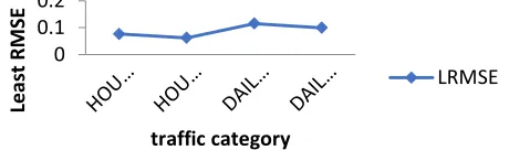
Table 1 and Fig. 2 present the least RMSE of the various traffic forecast categories based on the different traffic forecast design parameters. For the HOURLY_IN traffic, the least prediction RMSE was 0.076698 and it was observed on the parameters‘ combination of two hidden layers, 200
training epochs, and 24 input lags. For the HOURLY_OUT traffic, the least RMSE of 0.062199 was observed with parameters‘ combinations of 13 input lags, 200 training epochs on two hidden layers. 3 input lags, two hidden layers of 3 neurons each using 200 training epochs for predicting the DAILY_IN traffic recorded the least RMSE of 0.115213. For the DAILY_OUT traffic, 3 input lags, one hidden layer of three neurons with 200 training epochs had the least RMSE of 0.099416. The learning rate and momentum of 0.1 and 0.9 were respectively fixed for all experiments.
TABLE1
FORECASTING MODEL SELECTION FOR THE TRAFFIC
CATEGORIES
Hid den laye rs
Epo chs
Learn ing rate
Mo men tum
No of INP UT lags
Least RMSE
HOURLY _IN
2 200 0.1 0.9 24 0.076698 HOURLY
_OUT
2 200 0.1 0.9 13 0.062199 DAILY_I
N
2 200 0.1 0.9 3 0.115213 DAILY_O
UT
1 200 0.1 0.9 3 0.099416
Therefore, the selected traffic forecast model for the HOURLY_IN traffic was two hidden layers, 200 training epochs and 24 input lags; two hidden layers, 200 training epochs and 13 input lags for the HOURLY_OUT traffic category; two hidden layers, 200 training epochs and 3 input lags for the DAILY_IN traffic; and one hidden layer, 200 training epochs and 3 input lags for the DAILY_OUT traffic.
Fig 2. Summary least RMSE model selection of the traffic
categories
Fig. 2 revealed that various forecasting models may exist for different traffic categories, even if the traffic categories are all from the same network operator. This study has observed different forecasting models for the various traffic categories.
4.2 Evaluation of the Resource Provisioning of the Traffic Categories
Having determined the most appropriate predictive models for the Traffic categories, the study proceeded as follows In section 3, the required bandwidth estimation mechanism was formulated and presented in equation (5) as
Rt = ^
t
y(1+ α + d ) (16) 0
0.1 0.2
Least
R
M
SE
traffic category
331 where Rt is the estimate of the resource required at time t,
^
t
y is the volume of traffic predicted at time t, while d denotes neutralisation factor, and α is factor of safety to cater for sudden spikes and ensure smooth flow of traffic.
d
was derived by computing the percentage mean difference with respect to the desired traffic, as
1
1
( ( ) * 1 0 0 )
n
t t
t t
e c
d
n e
(17)
where et is the expected (desired) traffic load at time t and
ct, the computed (predicted) traffic load at time t.
The value which was defined as the margin of safety (some allowance), also referred to as factor of safety which the network manager or the operator wishes to add to make room for smooth flow of traffic, strictly depends of the level of satisfaction the network manager wishes and is ready to pay for. However, based on the recommendations 30% safety margin was used for this study.The neutralisation
factor d
, for each of the traffic category, were estimated using the historical traffic data collected for this study. Table
2 contains the d
value and bandwidth estimation model of the respective traffic at time t.
TABLE2
BANDWIDTH ESTIMATION MODELS FOR THE RESPECTIVE TRAFFIC
CATEGORY AT TIME T
Traffic Category d
value
Bandwidth Estimation at time t
HR_IN -0.06404 ^
(1 0 . 0 6 4 0 4 0 . 3 3 3 3 3 )
t
R t
y
HR_O -.1221214 ^
(1 0 . 1 2 2 1 2 0 . 3 3 3 3 3 )
t
R t
y
DA_IN - 0. 86447 ^
(1 0 . 5 8 6 4 4 7 0 . 3 3 3 3 3 )
t t
R y
DA_OUT ^
(1 0 . 1 5 4 5 7 3 0 . 3 3 3 3 3 )
t t
R y
The study compared
t
R with the expected traffic and
obtained -31.5% mean difference. This implied a guarantee of safety margin of about 31.5%, which was different from the specified 30% specified by 1.3 %. (31.5-30), the percentage of time the resource was inadequate for the traffic was 6.5%, while the percentage of adequacy of resource was 93.5%. For the HOURLY_OUT traffic, on applying the mechanism‘s predictive model, - 32.1723% mean difference was obtained between
t
R and the
expected traffic. This suggested a guarantee of safety margin of about 32.2%, which was different from the initial 30% specified by 2.2 %. The percentage of time the resource was in inadequate for the traffic was 9.1% while the percentage of adequacy of resource was 90.9%. This could be further improved by increasing the safety margin. Similarly, for the DAILY_IN traffic, by comparing Rt with the expected (actual) traffic, -31.4159 mean difference was
observed, that is, a guarantee of -31.4159% safety margin was obtained. This was different by 1.4 % from the 30% originally specified. The percentage of the number of times the resource was inadequate for the traffic flow was 12.85714 %. while the percentage of adequacy of resource was 87.1%. For the DAILY_OUT traffic, by using the selected predictive model, it was compared with the expected (actual) traffic and-27.7434% mean difference was observed, that is, a guarantee of 27.7434% % safety margin. This shows a 2.3 % difference from the 30% originally specified. The percentage of the number of times the resource was inadequate for the traffic flow was 44.28571%, while the percentage of adequacy of resource was 55.7%. This large percentage of under-provisioning implied that a larger safety margin might be required for this traffic category. However, the more the safety margin the more the cost of provisioning the resource.
4.3 Evaluation of the developed provisioning model with some existing formulae
Four variations of existing bandwidth provisioning models in [9]: The traditional provisioning formula, which computes by the mean traffic rate plus a margin of 30%, expressed as
t
R M M
(18) where M is the (expected) average traffic load, and denoting some factor that reflects the desired performance target P. For this experiment was set at 30%.
A generic formula which incorporates some error term into the traditional formula, express as
. t
R M V
(19)
where V is some error term to account for fluctuations of the traffic rate. For this study was set at 30%, and the
standard deviation, V a r , was the error term V .
(i) The bandwidth provisioning formula based on Gaussian counterpart of M /G / input:
t
R (20)
where denotes the long term mean traffic rate and, a
desired performance target. 30% was chosen for also chosen for .
A bandwidth provisioning formula based on generic Gaussian input, stated as
1
( 2 lo g ) . ( )
t
R v T
T
(21)
where T is a length of sample interval, the denotes some small value of fraction of T for which the offered traffic capacity exceeds the link capacity and v T( ) being the variance of traffic arrival.
The following provisioning estimates, shown in Table 3, were obtained respectively for the existing models,
TABLE3
REQUIRED BANDWIDTHESTIMATES OF THE EXISTING
FORMULAE IN KBITS/S
. t
R M M
t
R Rt M .V Rt 1 ( 2 lo g ). ( )v T
T
HR_IN HRY_O DA_IN DA_O
8459.16 3349.86 8833.46 3660.64
6531.25 2592.05 6668.84 2769.68
7336.28 2578.19 7076.37 3105.04
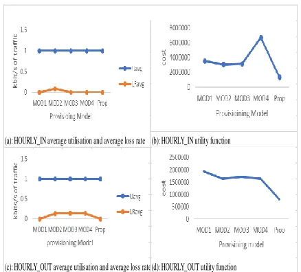
12035.28 2585.95 9276.04 3428.29 Fig. 3 shows the average utilisation, average loss rate and the utility function of HOURLY traffic categories with respect to the various provisioning models. For the HOURLY_IN, the models have the same average utilisation of 1, average loss rate of 0, except for model 2 (one of the existing models) that has an average loss rate of 0.086271935. The result implies that model 2 has the worst loss rate. The developed provisioning mechanism, represented by ‗prop‘ for proposed provisioning, recorded the least value (see Fig. 3 (b)):1312706 of the utility function. By implication it has the highest and most impressive utility compared to the other provisioning model.
Fig. 3. HOURLY traffic average utilisation, average loss
rate and utility function
For the HOURLY_OUT, the models have the same average utilisation of 1. The proposed estimation scheme and one of the existing models have average loss rate of 0. This implies that the propose model had the minimal loss rate, alongside with one of the existing models. This is an impressive result compared to the other models. Fig. 3 (d) gives the utility function of the various models of the HOURLY_OUT traffic set. The minimum value of 796952.8 was recorded again by the developed provisioning mechanism. This shows that the developed mechanism has a highly competitive advantage over the other models for this data set.Fig. 4: presents the average utilisation, average loss rate and the utility function of the DAILY traffic set. For the DAILY_IN traffic category, the models have the same average utilisation of 1, the same loss rate of 0, except for mode1 2 that has loss rate of 0.0090592. This implies that model 2 has the worst loss rate.
Fig. 4: DAILY traffic average utilisation, average loss rate
and utility function
The minimum value the utility function of the DAILY_IN traffic was recorded by MOD2, one of the existing models, with cost function of 829881.10, followed by MOD3, with 87201.47, the next to this was the developed model with the value of 99450.54 and lastly Model 1, with 162584.18. In terms of the utility function for this traffic set, the developed mechanism was outperformed by two of the existing models.Fig. 4 (c) shows the average utilisation and average loss rate of the DAILY_OUT traffic category. The models have the same value of the average utilisation of 1, the same loss rate of 0, except for mode1 2 that has loss rate of 0.076582132, and the developed mechanism with loss rate value of 0.000539374. By implication, the developed provisioning mechanism was only better than one of the existing models, MOD2. The utility function of the DAILY_OUT traffic set is represented in Fig. 4 (d). MOD1 records the highest cost function of 72697.73, followed by the developed mechanism, with the value of 72423.13. In terms of the utility function for this traffic set, the developed mechanism was outperformed by three of the existing models.
4.4 Discussion of the Findings
The result obtained from the proposed required bandwidth estimation was presented and compared with four provisioning methods in section 4. The metric employed were the average utilisation, which is computed as the ratio of the bandwidth utilised (bandwidth provisioned less current traffic rate) to the bandwidth provisioned; the average Loss Rate, which measures the bytes dropped at the interface due to under provisioning of bandwidth, and the utility function, which is used to evaluate the overall utility of the provisioning mechanism. For the HOURLY_IN and HOURLY_OUT traffic sets, the developed provisioning mechanism gave impressive results of the average utilisation, the lowest average loss rate and the minimum cost function, compared with the existing models. It gave the overall best utility of the provisioning, by recording the minimum value of the utility function. These could have stemmed from the learning capability incorporated in the model for representing the offered traffic and a factor for moderating over or under provisioning of resources. However, the performance of the developed mechanism was not so impressive compared with some of the existing models of the DAILY_IN and DAILY_OUT traffic categories. Its performance in terms of the average utilisation and average loss rate was impressively competitive with the (c): HOURLY_OUT average utilisation and average loss rate
(a): HOURLY_IN average utilisation and average loss rate (b): HOURLY_IN utility function
(d): HOURLY_OUT utility function
(c): DAILY_OUT average utilisation and average loss rate
(a): DAILY_IN average utilisation and average Loss Rate (b): Utility Function of the DAILY_IN
333 existing models, on the DAILY_IN traffic set, however, it
was outperformed by two of the existing models on the utility function for this traffic set. On the DAILY_OUT traffic categories, it was observed that the developed provisioning mechanism gave a highly competitive value of the average utility and average loss rate compared with the existing modes. However, it was outperformed by three of the existing models in terms of the utility function. On the overall the performance of the developed provisioning mechanism was better on the HOURLY traffic categories than that of the DAILY traffic sets. This could have been attributed to the large sample size of data used for the HOURLY_IN traffic sets. ANN performs better on large sample data sets than small sample sets [19] , [27] and [24]. The DAILY traffic bandwidth provisioning could be improved upon by deploying large margin of safety at the expense of high cost, say of 100% or above of the predictor. This study has shown that the better the traffic estimator the lower will be the margin of safety required and the lower the cost of provisioning; the worse the traffic estimator the higher the margin of safety required and the higher the cost of provisioning.
5
C
ONCLUSIONThis study proposed and tested an improved resource provisioning mechanism for bandwidth estimation. On the overall, the performance of the proposed scheme was highly impressive in comparison with the existing models. The study further revealed that an accurate traffic forecasting could reduce the cost of provisioning of resources. The better the traffic estimator the lower the required margin of safety and the lesser the cost of provisioning; the worse the traffic estimator, the higher the required margin of safety and the higher the cost of provisioning. The impressive performance of the result could be attributed to the learning capability of the technique employed, which could model the nonlinear and high degree of variability of internet traffic. This will be more useful in service delivery relating to finding solutions in healthcare and research resources involving disease activities[28-30]. Nevertheless, experimentation methods employed to determine the appropriate model for the forecasting component was highly computationally demanding. Therefore, efforts on developing methods for optimum determination of the ANN training parameters remain a worthwhile one. The study has provided an effective and efficient mechanism for required bandwidth resource estimation. The results of this study will effectively contribute to enhancing several internet management related tasks such as general resource management.
A
CKNOWLEDGMENTThe authors wish to thank Redeemer‘s University and Covenant University for providing an enabling environment for this research.
R
EFERENCES[1]. D. Prangchumpol, "A Network Traffic Prediction Algorithm Based On Data Mining Technique," World Academy of Science, Engineering and Technology, vol. 7, no. 7, pp. 999-1002, 2013. [2]. O. Osuagwu, S. Okide, D. Edebatu and U. Eze,
"Low and Expensive Bandwidth Remains Key
Bottleneck for Nigeria‘s Internet Diffusion: A Proposal for a Solution Model.," West African Journal of Industrial and Academic Research, vol. 7, no. 1, pp. 14-30, 2013.
[3]. Bandwidth Task Force Secretariat, "More Bandwidth at Lower Cost," University of Dar es Salaam, Dar es Salaam, 2003.
[4]. R. Hu, J. Jiang, G. Liu and L. Wang, "Efficient Resources Provisioning Based on Load Forecasting in Cloud," The Scientific World Journal, vol. 2014, pp. 1-12, 2014.
[5]. M. Alasmar and N. Zakhleniuk, "Network Link Dimensioning based on Statistical Analysis and Modeling of Real Internet Traffic," Cornell University Library, New York, 2017.
[6]. N. Piedra, J. Chicaiza, J. López and J. García, "Study of the Apllication of Neural Network in Internet Traffic engineering," in Sixth International Conference on Information Research and Applications, Varna, Bulgaria,, 2008.
[7]. A. Pras, L. Nieuwenhuis, R. v. d. Meent and M. Mandjes, "Dimensioning network links: a new look at equivalent bandwidth," IEEE Network, vol. 23, no. 2, pp. 5-10, 2009.
[8]. M. Crovella and B. Krishnamurthy, Internet Measurement: Infrastructure, Traffic and Applications, Wiley, 2006.
[9]. R. v. d. Meent, "Network Link Dimensioining: A measurement & modeling based approach," Centre for Telematics and Information Technology, University of Twente, Enschede, The Netherlands, 2006.
[10]. H. v. d. Berg, M. Mandje, R. v. d. P. A. Meent, F. Roijers and P. Venemans, "QoS-aware bandwidth provisioning for IP network links," Elsevier Computer Networks, vol. 50, no. 5, pp. 635-647, 2006.
[11]. R. d. O. Schmidt, H. v. d. Berg and A. Pras, "Measurement-based network link dimensioning," in 2015 IFIP/IEEE International Symposium on Integrated Network Management (IM), Ottawa, ON, Canada, 2015.
[12]. R. Ali and F. Zafar, "Bandwidth Estimation in Mobile Ad-hoc Network," International Journal of Computer Science Issues, vol. 8, no. 5, pp. 331-337, 2011.
[13]. S. S. Chaudhari and R. C. Biradar, "Survey of
Bandwidth Estimation Techniques in
Communication Networks," Wireless Personal Communications, vol. 83, no. 2, pp. 1425-1478, 2015.
[14]. P. Cortez, M. Rio, P. Sousa and M. Rocha, "Topology Aware Internet Forecasting using Neural Networks," in 17th International Conference on Artificial Neural Networks, Porto, Portugal, 2007. [15]. P. Cortez, M. Rio, M. Rocha and P. and Sousa,
"Internet Forecasting using Neural Networks," in International Joint Conference on Neural Network, Vancouver, 2006.
[17]. M. L. F. Miguel, M. C. Penna, J. C. Nievola and M. Pellenz, "New models for long-term Internet traffic forecasting using artificial neural networks and flow-based information,"in Proceedings of the 2012 IEEE Network Operations and Management
Symposium. , pp. 16-20, 2012.
doi:10.1109/NOMS.2012.6212033
[18]. S. Chabaa, A. Zeroual and J. Antari, "Identification and Prediction of Internet traffic using artificial neural networks," Intelligent Learning Systems & Applications, 2010.
[19]. S. Benkachcha, J. Benhra and H. El Hassani,
"Causal Method and Time Series
Forecastingmodel based on Artificial Neural Network," International Journal of Computer Applications, vol. 75, no. 7, pp. 37-42, 2013. [20]. G. Rutka and G. Lauks, "Study on Internet Traffic
Prediction Models," ELECTRONICS AND ELECTRICAL ENGINEERING, vol. 78, no. 6, pp. 77-50, 2007.
[21]. J. Faraway and C. Chattfield, "Times series forecasting with neural networks: a," Journal of Appl. Statistics, vol. 47, pp. 231-250, 1998. [22]. G. P. Zhang, B. E. Patuwo and M. Y. Hu, "A
Simulation Study of Artificial Neural Networks for Nonlinear Time-series Forecasting," Computer & Operations Research, vol. 128, pp. 381-396, 2001. [23]. H. Peng, J. Zhou, W. Liu, Z. X. and Y. Li, "Study on the Determination of Safety Factor in Calculating Building," in Procedia Engineering: The 5th Conference on Performance-based Fire and Fire Protection Engineering, Beijing, 2011.
[24]. G. Zhang, B. E. Patuwo and M. Y. Hu, "Forecasting with artificial neural networks: The state of the art," International Journal of Forecasting, vol. 14, p. 35 – 62., 1998.
[25]. S. Haykin, Neural Networks and Learning Machines, New Jersey: Pearson Education, Inc., 2009.
[26]. B. Krithikaivasan, K. Deka and D. Medhi, "Adaptive Bandwidth Provisioning Envelope based on Discrete Temporal Network Measurements," in IEEE INFOCOM, Hong Kong, 2004.
[27]. S. Islam, J. Keung, K. Lee and A. Liu, "Empirical prediction models for adaptive resource provisioning in the cloud," Future Generation Computer Systems, vol. 28, pp. 155-162, 2012. [28]. V. Osamor, E. Adebiyi, S. Doumbia, "Comparative
functional classification of plasmodium falciparum genes using kmeans clustering" in International Association of Computer Science and Information Technology - Spring Conference, IACSIT-SC 2009, pp. 491-495. 2009.
[29]. V. C. Osamor, "Experimental and computational applications of microarray technology for malaria eradication in Africa", Scientific Research and Essays, vol 4 no 7, pp. 652-664, 2009.