1504
Quantitative Comparison Of Reconstruction
Methods For Compressive Sensing Mri
T. Surya Kavita, Dr. K.Satya Prasad
Abstract : Magnetic Resonance (MR) Imaging is a non-invasive imaging system utilized generally for clinical diagnosis. MR imaging scanner gathers information in the form of Fourier coefficients and are stored in k-space. There are numerous algorithms to under sample k-space data using compressive sensing (CS) and to reconstruct the image. The under sampling pattern plays a critical role in optimizing compressed sensing MR imaging. In CS the signals are sampled at a rate much lower than traditional sampling rate and violate Nyquist’s criteria. CS MR imaging will reduce acquisition time by capturing only few samples. In this paper k-space information is under sampled with random sampling and reconstructed using different algorithms which are compared qualitatively and quantitatively. In reconstruction of brain MR image, Peak Signal- to-Noise Ratio (PSNR), Structured Similarity Index Measure (SSIM) and Mean- Square- Error (MSE) values are the fault prediction parameters. Based on quality of the visual image and its statistical analysis of the MR images, the Total Variation (TV) norm performed well over the other algorithms.
Index Terms: Compressive Sensing, MRI, MSE, PSNR, SSIM, TV
—————————— ——————————
1
INTRODUCTION
Medical imaging, now-a-days, has been evolved so predominant, involving the translation of details of each organ of patient’s body into a visual image. For diagnosing various diseases of a patient’s body, a medical imaging technique such as Magnetic Resonance Imaging (MRI) has been introduced. MRI is a new medical imaging model which produces an accurate and contented image of tissues and organs of a patient with the help of magnetic fields and radio waves [1]. The data or information acquired by MRI scanner is converted into a Visual Image by various recovery algorithms for the analyses of Medical practitioners. The data obtained by the MRI scanning machines is termed as k-space [2]. Acquisition Time of the MRI scanner is considered as an important parameter in data collection, and to match this scan acquisition time with the Nyquist rate, more data has to be collected based on the resolution of the image chosen. This made to evolve MRI recovery using partial k-spaces, minimizing the acquisition time, artifacts and patient’s exposure to the harmful Magnetic intensities [12][13]. The concept of Compressive Sensing (CS) ensures that sampling the signal down at very low rates than the Nyquist’s has an opportunity of better quality reconstruction. [3] [10]. In this paper, section 2 deals with the concepts of Compressive Sensing, and section 3 describes the recovery of CS MRI using various algorithms such as Basic Pursuit (BP), Orthogonal matching pursuit (OMP), Compressive Sampling Matching Pursuit (CoSaMP), Iteratively Re-weighted Least Squares Minimization (IRLS), Subspace Pursuit (SP) and Total Variation (TV). The performance criteria parameters such as PSNR, SSIM and MSE of the recovery algorithms are explained in section 4. Section 5 depicts the simulation results as a comparison of all reconstructive algorithms and followed by section 6 as conclusions.
2. COMPRESSIVE SENSING
In accordance with Shannon Nyquist theorem, sampling rate is atleast two times greater than the signal bandwidth for signal reconstruction. Compressed sensing Theory is based on sparse representation on signals, using small number of linear measurements. Mathematically, for reconstructing a sparse signal having a few non-zero coefficients, we need linear non-adaptive measurements which are observed from:
(1)
where, is a matrix, which is called sensing matrix and is a vector, called as observation vector.
Fig.1: Traditional Sampling
Fig.2: Compressive Sampling
Fig.1 and Fig.2 shows the concept of traditional sampling and Compressive Sampling (Sensing). Using CS theory, a signal can be reconstructed from samples less than Nyquist Rate [1], [2]. For exact recovery, the number of samples required relies on the recovery algorithm used. The image is transformed to sparse domain by using a sparse transform such as wavelet transform:
(2) Measurement Vector y
Signal
x Sampling Compression
No. of samples >> Information Rate
Number of samples is far less than that in the traditional sampling
Measurement Vector y
Signal
x Compressive Sensing
_________________________
T. Surya Kavita is a Research Scholar in ECE department , JNTU, Kakinada, India, E-mail: [email protected]
1505 IJSTR©2019
www.ijstr.org where, is a sparce transform. is sampled by mixing
with sampling matrix , which is stable and incoherence with the sparce transform:
(3)
where, the product is called the compressed sensing matrix 𝐴. 𝐴 , is called observation vector. The original image is reconstructed from this observation vector. In fidelity reconstruction, sparsity is the basic principle. Reconstruction algorithm using Compressed Sensing has the following steps:
i. Take sparse transformation for the signal . Here discrete wavelet transform (DWT) is used as sparse transform. Obtain .
ii. Design observation matrix M of dimensions m x n which is uncorrelated with the transform basis . Then obtain observation vector, .
iii. Reconstruct signal from using reconstruction algorithms such as orthogonal matching pursuit (OMP).
Figure 3 shows block diagram representation of compressive sensing reconstruction.
Fig. 3: Compressive Sensing Reconstruction
3 RECONSTRUCTION OF CS MRI
Compressive Sensing is a method to under sample image at a rate less than Nyquist’s rate and reconstruct the image from less number of samples. Reduction in the number of samples reduces image acquisition time. k-space data acquired by the MRI scanner is in the form of Fourier coefficients[14]. CS MRI under sample k-space by using under sampling techniques such as Cartesian, random and radial sampling. To get back the original MR image a reconstruction algorithm is to be applied. In the literature of MRI reconstruction, there exist numerous efficient algorithms for finding these coefficients of observation vector on iterations based instead of searching out ‘m’ highest coefficients at the same interval. Let the reconstructed image is represented by a complex vector m, let Ψ denote the sparse transform that transforms from pixel representation into a sparse representation. Let FS denote
the under-sampled Fourier transform. Reconstructions are obtained by solving the following constrained optimization problem [3]:
Minimize ‖ ‖ such that ‖ ‖ (4)
Where, is the measured k-space data from the MRI scanner and controls the fidelity of the reconstruction to the measured data. The threshold parameter is roughly the expected noise level. The reconstruction problem here
is to find a solution that is compressible by the transform among all solutions that are reliable with the acquired data. This paper compares the performance of various reconstruction algorithms.
3.1 Basis Pursuit
Basis Pursuit (BP) algorithm is a technique to solve ℓ1
minimization problem which is formulated as linear programming problem for compressive sensing. This approach is based on the convex ℓ1-minimization that
provides near optimal solution, can be defined as [4]: ‖ ‖ subject to (5)
Where ‖ ‖ ∑ | | is ℓ1 norm and ‖ ‖ is minimum
ℓ1 norm of . BP algorithm aims in decomposition of a
signal into a superposition of library components that have the smallest ℓ1-norm of the coefficients.
3.2 Orthogonal Matching Pursuit
Orthogonal matching pursuit (OMP) belongs to the group of greedy algorithms and overcomes the matching pursuit in many manners as it is simple and recovers the signal quickly. Identifying the position of largest ideal signal is the most important part in signal recovery. It uses an iterative approach, where a component is selected from a component library and approximates better with the residual. Instead of taking a scalar product of residual and the new library component to achieve the weight of coefficient, the actual function is to fix all picked library components through least squares by projecting the function orthogonally unto all picked library components [8].
3.3Compressive Sampling Matching Pursuit
Compressive Sampling Matching Pursuit (CoSaMP) algorithm is another stretch of the OMP algorithm having presumed to be a better one than the latter[9]. Similar to OMP, finding K largest components in x is the most challenging part. At each iteration, the algorithm finds largest 2K components of proxy and unite with index of the current signal approximation. Then it estimates the signal by using the least squares. Next, K largest components are selected as signal approximation to prune signal estimation.
3.4 Iteratively Re-weighted Least Squares Minimization
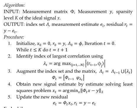
{ }|〈 〉|
[ ]
Algorithm:
INPUT: Measurement matrix , Measurement , sparsity level K of the ideal signal x.
OUTPUT: index set , measurement estimate , residual .
Procedure:
1. Initialize, , , , Iteration . While do
2. Identify index of largest correlation using
3. Augment the index set and the matrix, ⋃{ }
4. Obtain new signal estimate by estimate solving least squares problem ‖ ‖
5. Update the new residual
End while. Reconstructed
Signal
Signal x Sparse
Transform
Reconstruction Algorithm Compressive
1506
Algorithm:
INPUT: Measurement matrix , Measurement , sparsity level K of the ideal signal x.
OUTPUT: K-sparse estimate ̂, index set , signal estimate , residual .
Procedure:
1. Initialize, , , , Iteration .
2. While (halting criterion false) do . 3. Find the proxy of the current samples residual
4. Identify largest 2K components of proxy and unite with index of the current signal approximation.
5. Augment the index set ⋃
Iteratively Re-weighted Least Squares Minimization (IRLS) algorithm offers another alternative in directly getting a solution to ℓ1 minimization problem. A standard sparse
problem in restricted form can be solved by conventional IRLS algorithm [7]:
‖ ‖ subjected to (6)
In practice, ℓ1 norm is replaced by a reweighted ℓ2 norm
given by
subject to (7)
The solution of present iteration can compute the diagonal weight matrix W in ith iteration, in precise, from the diagonal components,
| | (8)
With present weights , the closed form solution for can be obtained as
(9)
3.5 Subspace pursuit
A contentious recovery algorithm named Subspace Pursuit (SP) is another CS algorithm having a recovery status very much higher when compared with ℓ1-minimization [5]. It has
low complexity than Matching Pursuit algorithms for sparse signal recovery. SP works well in both noisy and noiseless environments.
3.6 Total-Variation Minimization
Total variation indicates the integral of absolute gradient of the image. When applied in image reconstruction, excessive details in image have large total variation. Removing these details will reduce TV of the image and is close to the original image. In image processing, the aim of optimization is effectively utilized with a widely used TV norm, when limited variation occurrences are implemented for sparsifying transform. Even if another sparsifying transform is intended, it is typically helpful to incorporate a TV penalty as well. Such a combined objective seeks image sparseness each within the transform domain and the finite-differences domain, at the equal interval. In this regard the optimization can be given asminimize ‖ ‖ such that ‖ ‖ (10)
Where, is reconstructed image, is sparse transform, is total variation, is under sampled Fourier transform, is the threshold parameter and λ trades sparsity with limited-variations sparsity [6].
4
PERFORMANCE CRITERIA
To evaluate and compare the performance of various recovery algorithms of an MRI, a few regularized criteria were utilized by the researchers from the past. Three primary objective criteria used are: Peak Signal-to-Noise Ratio (PSNR), Structured Similarity Index Measure (SSIM) and Mean Square Error (MSE). They are used to evaluate the performance comparison of different reconstruction algorithms. PSNR is the most widely used objective criterion for evaluating the quality of images and is defined as
(11)
where, is the maximum pixel value. For an 8-bit image L is 255 and for good reconstruction PSNR is high.
SSIM stood for many years as a measurement of evaluating the reconstructed image quality with the help of a reference image. If two images reference and reconstructed, having local windows of a and b respectively, then SSIM is given as
(12)
where, , stand for the intensity mean values of a and
b, and , stand for variance values of a and b respectively. Subsequently, the constants and are introduced to eradicate the unstableness caused when SSIM denominator approaches zero. Its range starts at no correlation value of 0 to a complete correlation value of 1.From the quantitative perspective, MSE can be a great measure; however, it can easily become misleading. When MSE is used within the same type of image artifact, it is great at distinguishing between small levels of error. It gives the squared difference between the actual image and reconstructed image.
} ̃ ⋃
̃} Algorithm:
INPUT: measurement matrix Φ, measurement y, sparsity level K of the ideal signal .
Initialization : , .
Iteration : Follow the below steps at the ith iteration 1. {
2. ̃ {‖ ‖ ̃} 3. {
4. {‖ ‖ } 5. Until the stopping criteria is met.
Output: , supp( )
( )
Algorithm:
INPUT: Measurement matrix , Measurement , ideal signal x.
While the halting criterions do not meet Update W: | |
Update X: ( ) Update
1507 IJSTR©2019
www.ijstr.org (13)
Here represents input or original image and represents output or reconstructed image. k and l are position of pixel in an image.
5
SIMULATION RESULTS
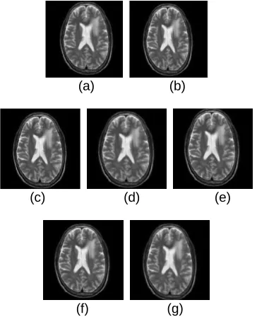
The simulation results performed using MATLAB tool for the MRI reconstruction is depicted in this section at 75% sampling using various methods. Compressive sensed MRI is reconstructed using various algorithms and all the algorithms are tested on 256 × 256 brain image. Actual MR brain image and reconstructed images using different algorithms are shown in Fig.4. MR image is converted into sparse domain by using DWT, and then under sampled using random sampling to achieve CS. The Quality of the reconstructed MR image is evaluated with the help of PSNR and MSE. The calculations of the differences are taken over the actual MR image and reconstructed one. A high image quality ensures from a low value of MSE while a high PSNR value indicates a greater quality of image.
(a) (b)
(c) (d) (e)
(f) (g)
Fig. 4: Compressive Sensing Reconstruction using various algorithms (a) Actual image (b) reconstructed using TV (c)
OMP (d) CoSaMP (e) IRLS (f) BP (g) SP
SSIM helps in evaluating the amount of correlation between two images. This is formulated to enhance on ancient methods namely PSNR and MSE, which estimate absolute errors. SSIM is indexed in a complete reference metric and compares pixel intensity local patterns that were normalized for contrast as well as luminance [11].
Table I: Values of PSNR, SSIM and MSE at 75% sampling for reconstructed MR images
Method PSNR SSIM MSE
BP 32.1674 0.9085 29.2340 OMP 28.3968 0.8565 75.7036
CoSaMP 28.8224 0.8594 66.9217 TV 36.5136 0.9495 11.8554 SP 29.0521 0.8687 58.8423 IRLS 33.6198 0.9177 23.8911
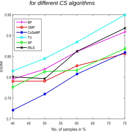
Table I gives the values of PSNR, SSIM and MSE at 75% sampling for reconstructed MR images. SSIM for TV minimization reads as 0.9495 indicating the value very near to that of the actual image. Fig. 5 represents the curves of comparison for the algorithms at number of samples in percentage of 40, 50, 60 and 75. It is observed that the TV norm provides better results compared with its counter parts in case of PSNR. Fig. 6 represents MSE comparison between the discussed algorithms for different sampling percentage. As shown, MSE values are lower for the TV algorithm as compare to other. Hence, the TV algorithm provides better reconstruction. Fig. 7 gives the SSIM comparison between the algorithms for different sampling levels. It is clearly visible that SSIM for TV is better than other, as SSIM approaches to higher values compare to other methods. Performance can be further improved by using a better sparse transform and combining different reconstruction techniques.
Fig. 5: Sampling rates versus PSNR Comparison for different CS algorithms
∑ ∑
1508
Fig. 6: Sampling rates versus MSE Comparison for different CS algorithms
Fig. 7: Sampling rates versus SSIM Comparison for different CS algorithms
6
CONCLUSION
Compressed sensing concept is reviewed and MRI reconstruction is carried out using BP, OMP, CoSaMP, TV, SP and IRLS algorithms in this paper. Based on the experimental results, it is observed that the TV norm algorithm provides better reconstruction compare to BP, OMP, CoSaMP, SP and IRLS. OMP and CoSaMP, BP and IRLS are almost equally efficient in the MR image reconstruction. A good result at a very sampling is given by this reconstruction process. Nevertheless the quality in image differences becomes huge at a very less sampling percentage. Hence by integrating the non linear techniques of reconstruction such as ℓ1 minimization and TV minimizing methods having optimization algorithm like Particle swarm optimization (PSO) increases the overall performance.
REFERENCES
[1] D.L.Donoho: Compressed sensing. IEEE Transactions on Information Theory, 52:1289-1306, (2006).
[2] Candes E.J, Wakin M.B: An Introduction to Compressive Sampling. IEEE Signal Processing Magazine, Vol.2 (5), (March 2008).
[3] E.Candes, J.Romberg: Sparsity and incoherence in compressive sampling. Inverse Problems, Vol.23, p.969, (2007).
[4] Sujit Kumar Sahoo and Anamitra Makur: Signal Recovery from Random Measurements via Extended Orthogonal Matching Pursuit. IEEE transactions on signal processing, vol. 63 (10), (May 2015).
[5] Chao-Bing Song, Shu-Tao Xia, and Xin-Ji Liu: Improved Analysis for Subspace Pursuit Algorithm in Terms of Restricted Isometry Constant. IEEE Signal Processing Letters, Vol. 21 (11), (Nov 2014).
[6] Shiqian Ma, Watao Yin and Amit Chakraborty: An Efficient Algorithm for Compressed MR Imaging using
Total Variation and Wavelets. IEEE Conference on Computer Vision and Pattern Recognition, pp.1-8, (2008).
[7] Chen Chen, unzhou Huang, Lei He, and Hongsheng Li: Fast Iteratively Reweighted Least Squares
Algorithms for Analysis-Based Sparsity
Reconstruction. IEEE Transactions on Pattern Analysis and Machine Intelligence, Vol. XX, (April 2015).
[8] J.A.Tropp and A.C.Gilbert: Signal recovery from random measurements via orthogonal matching pursuit. IEEE Transactions on Information Theory, vol. 53 (12), pp. 4655–4666, (Dec. 2007).
[9] Carrillo, Rafael E. et al.: Iterative algorithms for compressed sensing with partially known support. IEEE International Conference on Acoustics, Speech and Signal Processing, pp. 3654-3657, (2010).
[10] Lustig M., Donoho D. and Pauly J.M.: Sparse MRI: The application of compressed sensing for rapid MR imaging. Magnetic Resonance in Medicine, vol.58, pp.1182-1195, (2007).
[11] Zhou Wang, A. C. Bovik, H. R. Sheikh and E. P. Simoncelli: Image quality assessment: from error visibility to structural similarity. IEEE Transactions on Image Processing, vol. 13, no.4, pp.600-612, (April 2004).
[12] J. Huang, Zhang S., Metaxas D.: Efficient MR image reconstruction for compressed MR imaging. Medical Image Analysis, vol.15 (5), pp.670-679, (2011). [13] J. P. Haldar, D. Hernando and Z.P. Liang:
Compressed-sensing MRI with random encoding. IEEE Transactions on Medical Imaging, vol. 30 (4), pp. 893–903, (2011).