Article
Landslide Susceptibility Mapping at Two Adjacent
Catchments Using Advanced Machine Learning
Algorithms
Ananta Man Singh Pradhan 1 and Yun-Tae Kim 2,*
1 Water Resource Research and Development Centre, Ministry of Energy, Water Resources and Irrigation,
Government of Nepal, Pulchok, Lalitpur, 44600, NEPAL; [email protected]
2 Department of Ocean Engineering, Geo-Systems Engineering Laboratory, Pukyong National University, 45
Yongso-ro, Nam-gu, Busan, 48513, KOREA; [email protected] * Correspondence: [email protected]
Received: 2 August 2020; Accepted: date; Published: date
Abstract: Landslides impact on human activities and socio-economic development especially in mountainous areas. This study focuses on the comparison of the prediction capability of advanced machine learning techniques for rainfall-induced shallow landslide susceptibility of Deokjeokri catchment and Karisanri catchment in South Korea. The influencing factors for landslides i.e. topographic, hydrologic, soil, forest, and geologic factors are prepared from various sources based on availability and a multicollinearity test is also performed to select relevant causative factors. The landslide inventory maps of both catchments are obtained from historical information, aerial photographs and performing field survey. In this study, Deokjeokri catchment is considered as a training area and Karisanri catchment as a testing area. The landslide inventories content 748 landslide points in training and 219 points in testing areas. Three landslide susceptibility maps using machine learning models i.e. Random Forest (RF), Extreme Gradient Boosting (XGBoost) and Deep Neural Network (DNN) are prepared and compared. The outcomes of the analyses are validated using the landslide inventory data. A receiver operating characteristic curve (ROC) method is used to verify the results of the models. The results of this study show that the training accuracy of RF is 0.757 and the testing accuracy is 0.74. Similarly, training accuracy of XGBoost is 0.756 and testing accuracy is 0.703. The prediction of DNN revealed acceptable agreement between susceptibility map and the existing landslides with training and testing accuracy of 0.855 and 0.802, respectively. The results showed that, the DNN model achieved lower prediction error and higher accuracy results than other models for shallow landslide modeling in the study area
Keywords: Deep Neural Network; Extreme Gradient Boosting; Random Forest; Landslide Susceptibility
1. Introduction
Landslide and debris flow are one of a major natural hazard worldwide due to unfavorable geological causes, weathering patterns, shallow soil deposit and heavy rainfall. Landslides created dangerous menaces to the environment. The Korean peninsula is currently experiencing climate change effects, including annual temperature, precipitation and rate of typhoon occurrence [1]. Shallow seated landslides have often resulted from heavy downpour accompanying typhoons and torrential rains during the summer season (Kim and Lee, 2013).
Landslide prediction is a crucial task because the inherent causes of landslide are complex due to mechanical and chemical weathering, nonhomogeneous soil deposit, orientation of geological lineament, and erosion of a slope. The external causes including rainfall, earthquakes, and the excavation of a slope, and the loading of a slope or its crest are the most powerful agents to trigger
the landslide [4–8]. In the Korean Peninsula, one of the main causes of heavy downpour is a typhoon. Every year large-scale typhoons pass over South Korea, leaving a trail of devastation in its path.
Landslide susceptibility is the occurrence of a probability of landslide under certain
geo-environmental conditions and it estimates “where” landslides are most likely to occur in the future
[9,10]. In the last three decades, various researchers have proposed and applied GIS-based qualitative and quantitative methods [11]. The qualitative methods are subjective and depend on expert
decisions [12–14] and quantitative methods are objective and founded on the geographical
distribution of landslide and influencing factors (IFs). The weight of evidence, frequency ratio, relative effect models, logistic regression models have been frequently used in quantitative methods
[15–19]. In recent years, machine learning techniques have been increasingly employed for resolving
the non-linear spatial relationship with landslide occurrences, using either regression or classification methods [20–25].
Advances in computational technologies and the rapid development of advanced machine learning algorithms have amended the understanding and management of many geo-environmental problems. The main advantage of machine learning over traditional techniques is its capability to handle high-dimensional and complex non-linear datasets [26]. Various previous investigators have utilized machine learning in different fields of geosciences and hydrogeology, including spring potential mapping [27], gully erosion mapping [28], flood hazard mapping [29] and landslide studies [30,31]. Application of advanced machine learning algorithms to the landslide susceptibility modelling has been very limited despite their varieties and potential advantages.
The main aim of this research is to evaluate landslide susceptibility based on machine learning techniques i.e. Random Forest (RF), Extreme Gradient Boosting (XGBoost) and Deep Neural Network (DNN) in Deokjeokri and Karisanri catchments. The designed issue of this study is landslide susceptibility mapping with training the model in Deokjeokri catchment and testing the model in Karisanri catchment close to Deokjeokri catchment. Two adjacent catchments (Deokjeokri and Karisanri) were selected as study sites because two sites have similar geological and geomorphological settings and they had severe rainfall-induced landslide problems.
2. Description of study area
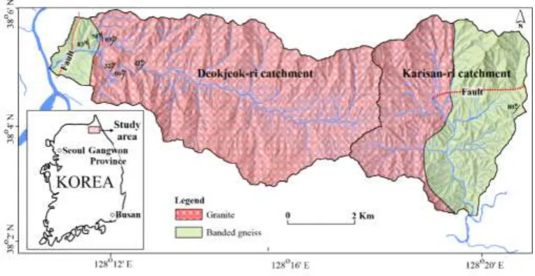
Deokjeokri catchment and Karisanri catchment are located within the Inje region, Gangwon Province in the northeastern part of Korea (inset of Figure 1). Deokjeokri catchment occupies about
33.4 km2, and Karisanri catchment about 22.2 km2. These catchments are confined by moderate to
Figure 1. Geological map of study area. The study sites are predominated by Mesozoic granites (Pink in color in Figure). Location of study area in inset.
3. The collected dataset and methods
3.1. Landslide inventory
A landslide inventory map records the geographic location, size, date, and type of landslide [33–
37]. The precise detection of landslide emplacements is crucial for the prediction and assessment of the landslide susceptibility models. A new generation of satellite images like Word view, Geo-eye aided a quick reproduction of landslide inventory maps [38]. Recently, the application of interferometry techniques to radar images is extensively used in inventory mapping [39]. However, due to the limitation of resources, in this study, we: (1) examined aerial photographs (provided in the web portal site: www.map.daum.net, www.map.naver.com) to prepare a landslide inventory map.
Both web portals give an excellent bird’s eye view with a 25 cm resolution. And (2) performed
fieldwork. The field observations showed that the predominant mass movements are shallow slides that sometimes ensued as debris flows during periods of heavy rainfalls and occurred on natural and man-made slopes with highly weathered bedrock.
As shown in Figure 2, a total of 748 landslides were identified and afterward digitized in ArcGIS 10.3 environment for further analysis in Deokjeokri catchment (training area) and 219 landslides were identified at Karisanri catchment (testing area). Some glimpses of landslide observed during field visits are presented in Figure 3. In this study, a single pixel from the center of each landslide initiation area was extracted. A Gaussian Kernal density function of sampling strategy (an unbiased sample technique) was used [40] for non-landslide pixels. A double number of non-landslide pixels (i.e. 1496 from Deokjeokri and 438 from Karisanri) were sampled in each catchment.
(a) (b)
(c) (d)
(e) (f)
Figure 3. (a)– (e): observed landslides and f) debris deposit.
3.2. Landslide influencing factor (IF)
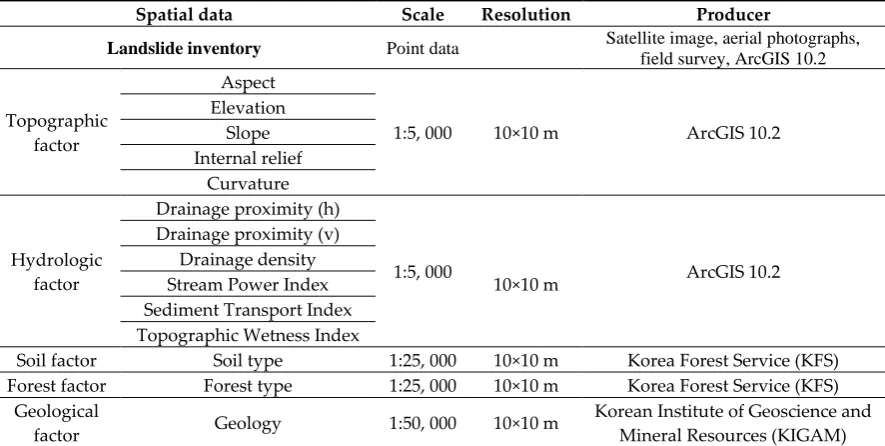
intrinsic factors such as topographic, hydrologic, forest, soil and geological factors, which are collected from available resources and fieldworks. Table 1 represents the spatial database obtained from different sources. In this study, based on reviewing previous researches [3,22,23,42] and availability of data, 14 IFs were utilized to identify the hillslope features of landslide occurrence. Among 14 IFs, topographic (except aspect map) and hydrologic factors are continuous but forest, soil, and geology are categorical factors. The selection of an appropriate pixel is necessary to achieve high precision in landslide susceptibility mapping [43,44]. Tarolli and Tarboton (2006) found that 10 × 10 m resolution is adequate to get better landslide susceptibility prediction performance so that 10 × 10 m resolution digital elevation model (DEM) was created from 5 m interval contours. Similarly, all collected IFs (thematic layers) were rasterized in 10×10 m pixel size.
Table 1. Data type, scale and producer.
Spatial data Scale Resolution Producer
Landslide inventory Point data Satellite image, aerial photographs, field survey, ArcGIS 10.2
Topographic factor
Aspect
1:5, 000 10×10 m ArcGIS 10.2
Elevation Slope Internal relief
Curvature
Hydrologic factor
Drainage proximity (h)
1:5, 000 ArcGIS 10.2
Drainage proximity (v) Drainage density
Stream Power Index 10×10 m
Sediment Transport Index Topographic Wetness Index
Soil factor Soil type 1:25, 000 10×10 m Korea Forest Service (KFS) Forest factor Forest type 1:25, 000 10×10 m Korea Forest Service (KFS)
Geological
factor Geology 1:50, 000 10×10 m
Korean Institute of Geoscience and Mineral Resources (KIGAM)
3.2.1. Topographic factors
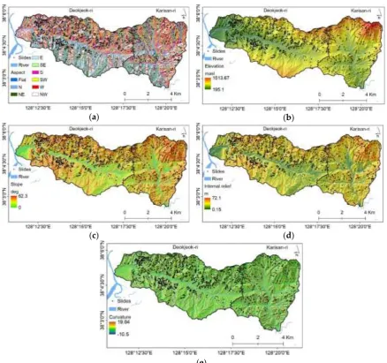
The aspect does not show a direct relation with landslide occurrence, however, the slope aspect of the terrain is related to parameters such as sunlight exposure and precipitation [45,46]. The aspect was divided into north, northeast, east, southeast, south, southwest, west, northwest and flat, as shown in Figure 4a. The elevation is another important element in landslide studies. Study shows that higher altitude tends to cause landslides [45]. The elevation of study area ranges from 195.1 to 1513.67 m asl as presented in Figure 4b. The slope is a very powerful driver of the landslide. In fact, the slope affects the surface and subsurface flow and thus the soil moisture content, soil formation and the likelihood of soil erosion (Cooke and Doornkamp, 1974). In the study area, the slope ranges
(a) (b)
(c) (d)
(e)
Figure 4. Topographic influencing factors: a) aspect, b) elevation, c) slope, d) internal relief and e) curvature.
3.2.2. Hydrologic factors
Hydrological factors are vital factors in rainfall-induced slope instability. Two types of drainage proximity, i.e. horizontal and vertical IFs were used in this study. The drainage proximity (h) (Figure 5a) was obtained from the Euclidean function in the GIS environment. A new topo-hydrological factor i.e. drainage proximity (v) was used. It gives the height above the nearest drainage network (Figure 5b). This index considers the height-differences along flow paths. Drainage density is the length of the drainage within a pixel (Figure 5c). The presence of higher drainage density means less percolation but faster surface flow [50].
The SPI indicates the erosive processes, as caused by runoff. As the specific catchment area and
slope gradient increase, the measure of water contributed by upslope and the surface runoff also increases [51]. Eq. (1) defines the SPI
s
SPI
=
A
tan β
, (1) where As is the specific catchment area, and β is the slope gradient. The spatial distribution of SPI is
(a) (b)
(c) (d)
(e) (f)
Figure 5. Hydrologic influencing factors: a) drainage proximity (h), b) drainage proximity (v), c) drainage density, d) SPI, e) STI, and f) TWI
The STI reflects the erosive power of the overflow drain and the process of erosion and deposition. To calculate STI, two components of the slope which are responsible for soil loss i.e. length (L) and steepness (S) were considered, as suggested by Moore and Burch (1986), given in Eq. (2)
0.6 1.3
s
A
sinβ
STI
22.13
0.0896
=
(2)where Asis the specific catchment area, and β is the slope gradient. The spatial distribution of STI is
shown in Figure 5e.
TWI is related to soil conditions and surface runoff [53]. TWI is the tendency of water to aggregate in the catchment and the propensity of gravitational powers to move downslope [54]. TWI is defined as
α
TWI
log(
)
tanβ
=
(3)where α is the cumulative upslope area, andβ is the slope angle. The distribution of TWI in the study
3.2.3. Forest and soil factors
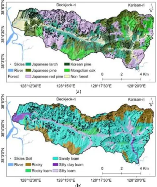
Rickli et al. (2002) addressed the effect of forest in hillslope reinforcement. The crucial role of trees and forests is to forestall mass movements by fortifying and drying soils. The catchments mainly consist of oak, Japanese larch, Japanese red pine, Japanese pine, and Korean pine forest as shown in Figure 6a. The non-forest area consists of agricultural land.
Soil properties affect degrees of drainage and erosion, which influence the landslide occurrence. The particle size and pore distribution affect water movement and the holding of infiltrated water (Kitutu et.al., 2009). Finer soils can hold higher volumes of water than coarse-textured soils [57]. In the study area, predominant soil types are sandy loam soils (Figure 6b). However, downstream areas were covered by silty clay loam and clay loam. The northern and southern elevated areas of the catchments are rocky and covered by a very thin layer of soil.
(a)
(b)
Figure 6. Influencing factors: a) Forest type and b) soil type
3.2.4. Geologic factor
3.3. Modeling approaches
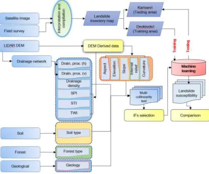
As illustrated in Figure 7, the fundamental working phases of adopted methodology in this study comprises four main steps: 1) preparation of landslide inventory and related database, 2) preparation of training and testing dataset, in this research Deokjeokri catchment was selected as a training area and Karisanri catchment a testing area, 3) landslide Ifs were tested and selected using multicollinearity test, and 4) preparation and comparison of performance of landslide susceptibility maps using RF, XGBoost and DNN models.
Figure 7. Illustrating study flow.
The quality of the predictions was examined using receiver operating characteristic curve (ROC) technique. The machine learning methods that applied in the present study are briefly described below:
3.3.1. Random Forest (RF)
Random Forest (RF) introduced by Breiman in 2001, has demonstrated to be an incredible
method in classification and regression. It has the ability to deal with high–dimension, continuous
and categorical data. RF does not require the assumption about the statistical distribution of the data and it can be considered robust with respect to changes in the composition of the dataset [60]. These properties are very useful in applications using variables that have mutual nonlinear interactions. In
this work, we used the “ModelMap” package [61] in R-statistical environment. The “ModelMap”
regression. After training, a prediction for a query points x, each tree independently predicts as given in Eq. (4) and (5)
( )
1
( )
(
( ))
i ni
j
n e i
Y A x n
I e
f
x
Y
N
A x
=
=
(4)
And the forest averages the predictions of each tree
( ) 1
1
( )
( )
M M j n n jf
x
f
x
M
==
(5)
Where
A x
n( )
denotes the leaf containing x andN A x
e(
n( ))
denotes the number of estimation points it contains.3.3.2. Random Forest (RF)
The XGBoost is based on the Gradient Boosting concept. It uses a more regularized model formalization to control over-fitting, which gives it better performance. It was developed by Chen
and Guestrin (2016). In XGBoost, training is done using an additive strategy. Given samples I with
independent Ifs data X1, X2,…..,Xn, a tree ensemble model uses K additive function to predict the outputs Y.
1
( )
( ),
K
i i k i k
k
Y
x
f x
f
F
=
=
=
(6)
where F is the set of all possible trees. The
f
kis a function at each of the k steps of the descriptorvalues in
x
ito a certain output. The differentiable loss function that measures the difference between the predictions and the target is simply a mean-square error. After each step of boosting, the algorithm scales the newly added weights. In this study, an open source code “xgboost” for R -environment was utilized [63].3.3.3. Deep Neural Network (DNN)
DNN is inspired by information processing and communication pattern in the biological nervous system [64,65]. In DNN, layers representations are learned via models called a neural network. From a technical point of view, DNN algorithms are multilayered neural networks. The main body of DNN consists an input layer that receives the data, an output layer that gives the prediction and core part is the hidden layer that processed the data. With the rapid development of DNN, a great number of libraries and packages have been developed to set a DNN with minimal
effort. In this work, we used the “keras” [66] and “H2O” (LeDell E et.al 2018) packages designed for
the R-statistical environment and runs seamlessly on both ‘CPU’ and ‘GPU’ devices.
4. Results and analysis
4.1. Selection of Ifs
The number of Ifs can be minimized via multicollinearity testing, reducing high-dimensional data. For the susceptibility analysis, the Ifs were examined through a multicollinearity test which is useful to select applicable Ifs. The variance inflation (VIF) and tolerance (TOL) are two indicators of the level of multicollinearity [67,68]. A VIF esteem more prominent than or equivalent of 10 and a TOL esteem under 0.5 demonstrates a genuine multicollinearity issue [69,70]:
2
TOL 1= −R (7)
where the coefficient of determination (R2) is the proportion of the variance in the target variable [71–
73]. The result is presented in Table 2, which shows that IR has a multicollinearity problem. So, IR was eliminated for further analysis.
Table 2. Multicollinearity test.
Statistic R² Tolerance VIF
Aspect 0.05 0.95 1.05
Elevation 0.40 0.60 1.67
Slope 0.70 0.30 3.33
Internal relief 0.90 0.10 10.47
Curvature 0.49 0.51 1.95
Drain prox. (h) 0.45 0.55 1.82 Drain prox. (v) 0.55 0.45 2.23 Drainage density 0.52 0.48 2.10
SPI 0.71 0.29 3.45
STI 0.78 0.22 4.55
TWI 0.74 0.26 3.85
Forest 0.25 0.75 1.33
Soil 0.02 0.98 1.02
Geology 0.09 0.91 1.09
Remark: Bold numbers are failed the multicollinearity test.
4.2. Application of RF in landslide susceptibility mapping
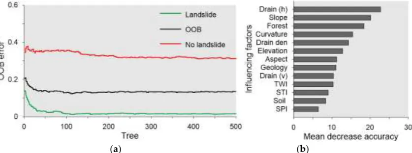
Three training parameters are needed to be defined in the RF model; ntree, the number of bootstrap samples for the original data (the default value is 500); mtry, the number of different predictors tested at each node i.e. as many as the IFs; node size, the minimum size of the terminal nodes of the trees [74]. The elements not included in ntree bootstrap sample are referred to as out-of-bag data (OOB) for that bootstrap sample. OOB is used to estimate an error rate called OOB error rate (Figure 8a). The result suggests that when the training of the data was applied to build the model, the error rates stay constant after 100 trees.
The error rate found to be 12% therefore 88% of the model building result was accurate, which makes this a reasonably good model. Figure 8b depicts the variable importance by means of the mean decrease accuracy in percentage. The result shows that drainage proximity (h) has the highest importance followed by slope and forest.
(a) (b)
4.3. Application of XGBost in landslide susceptibility mapping
Basic training using XGBoost is the most critical part of the modeling. It contains several hyper-parameters to be set [75]. We hold the trees constant at the default of 1000 rounds. The learning rate was selected as 0.1 to avoid overfitting the model. And the maximum depth of the tree was chosen as 3. Figure 9a shows the log loss during the modeling process. After tuning the model, it was found that the log loss of training process is 0.48 and log loss for testing data is 0.56 in 90 iterations, respectively. The model has the capability to check the important variables using bias of all IFs. Figure 9b illustrates that drainage proximity (h) is the most important IF followed by slope and curvature during the XGBoost modeling.
(a) (b) Figure 9. a) Loss vs iteration of XGBoost model and b) variable importance.
4.4. Application of DNN in landslide susceptibility mapping
There is no universal rule for the determination of an optimum neural net structure. In this study, 3 hidden layers and 13 neurons in each hidden layer were used. The input IFs were normalized
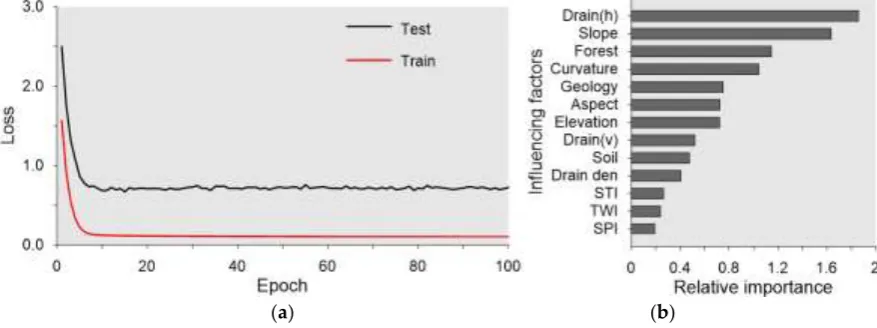
and then a “relu” activation function was used to run the model. The loss function is an important output of the model, which is used to measure the inconsistency between the dependent variable and the predicted outcome. Figure 10a presents the loss function during the modelling process. It has been found that as the number of epoch increases, the loss value for the training and test data decrease. After 10 epochs, the curves were stable. The relative importance of the model is presented in Figure 10b. Drainage proximity (h) is the most important IF followed by slope and forest.
(a) (b) Figure 10. a) Loss vs epoch of DNN model and b) variable importance.
4.5. Evaluation measures
(a)
(b)
(c)
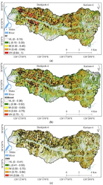
Figure 11. Landslide susceptibility maps: a) RF, b) XGBoost and c) DNN
susceptibility of a landslide occurrence. The high susceptible area is more confined near to the drainage and steep areas. The flat and gentle slopes represent the low susceptible areas.
One of the popular methods for model assessing accuracy is a receiver operating characteristic curve (ROC) in landslide susceptibility assessment. The ROC is a useful method to describe the quality of probabilistic prediction systems [76]. The area under the curve can be utilized as a measurement to evaluate the general execution of the model [77] with the goal that the bigger the area is, the better the presentation of the model becomes. A rough guide for grouping the exactness is the customary scholastic point framework. The following rankings were considered for accuracy test [78]: 0.90 – 1 (excellent), 0.80 – 0.90 (good), 0.70 – 0.80 (fair), 0.60 – 0.70 (poor) and 0.50 – 0.60 (fail).
The ROC evaluation for the three methods in the landslide susceptibility mapping shows that the area under the curve (AUC) values of training data are 0.757 (fair), 0.756 (fair) and 0.855 (good) for RF, XGBoost and DNN respectively (Figure 12a). Similarly, the AUC values of testing data are 0.74 (fair), 0.703 (fair) and 0.802 (good) for RF, XGBoost and DNN respectively (Figure 12b).
(a) (b)
Figure 12. Accuracy assessment using ROC: a) training and b) testing.
The comparison of the three methods shows that the prediction capabilities of these models are different. Among the three models DNN shows the highest prediction capability, followed by XGBoost and then RF model.
In order to compare the reliability of the obtained landslide susceptibility maps, a difference in the three landslide susceptibility methods was evaluated in a 2×2 contingency table. The number of correctly predicted landslides and non-landslides are indicated by TP (True positives) and TN (True negatives), and the number of incorrectly predicted landslides and non-landslides are FN (False negatives) and FP (False positives), respectively. The aim of two-class prediction methods is to separate true cases from false ones. Based on the four descriptors, several further measures can be calculated. Sensitivity also called true positive rate (TPR), and specificity (true negative rate, TNR) shows the ratio of the landslide and non-landslide cases correctly identified by the landslide susceptibility models. Positive predictive value (PPV) (also called precision) and negative predictive value (NPV) is the conditional probability that a landslide or non-landslide variant is predicted as landslide or non-landslide, and accuracy (ACC) is the correctly classified index, respectively. The mathematical basis of these parameters [79] are given as in equations (9)–(13):
TP
Sensitivity
TP
FN
=
+
(9)TN
Specificity
FP TN
=
TP PPV
TP FP
=
+ (11)
TN NPV
FN TN
=
+ (12)
TP TN ACC
TP FP FN TN
+ =
+ + + (13)
The results during the training and testing stages for implemented models are presented in Table 3, which clearly shows that the execution of all models produced very good outcomes. During training and testing phases, the correctly captured presence of landslides (TP) and absence of landslides (TN) are higher in DNN model than RF and XGBoost models. The ACC of DNN shows 74.01% (training phase) and 83.71% (testing phase), on other hand, 68.52% (training) and 74.73% (testing) for XGBoost and 67.28% (training) and 68.19% (testing) for RF model respectively. Performance results show the prediction of probable occurrence of landslide by DNN model surpasses the remaining models by significant tolerance followed by XGBoost and RF.
Table 3 Performance results of implemented models in the training and testing phases.
Data set Model TP FP FN TN Specificity (%) Sensitivity (%) PPV (Precision) NPV (Conditional probability) ACC (%) Training
RF 487 473 261 1022 68.36 65.36 50.73 79.66 67.28
XGBoost 493 451 255 1044 69.83 65.91 52.22 80.37 68.52
DNN 566 401 182 1094 73.18 75.67 58.53 85.74 74.01
Testing
RF 155 145 64 293 66.89 70.77 51.67 82.07 68.19
XGBoost 159 106 60 332 75.79 72.6 60.00 84.69 74.73
DNN 184 72 35 366 83.56 84.01 71.88 91.27 83.71
TP=True positive, FP=False positive, FN=False negative, TN=True Negative, PPV=Positive predictive value, NPV=Negative predictive value, ACC=accuracy
5. Discussion
Although the applied machine learning models are “black box model”, applying machine
learning is a field with a growing interest in recent years. The prescient outcomes do not distinguish the reasons for the landslide, however show the relation between landslides and terrain features. Nevertheless, such results may yield understanding into landslide events and which IF affect landslide in the study area. To get more definitive results, more experiments should be done to validate the model with time series landslide inventories.
Previous studies illustrated that RF method can adequately depict probable occurrence of landslide and spatial data [81,82,86,87]. There are several pieces of research on landslide susceptibility using a gradient boosting algorithm [88–90]. It was found that the Boosted model has better performance than the RF model. Recently, DNN is becoming popular among researchers [91,92]. Wang et al. (2017) has stated that DNN framework achieved higher or comparable prediction accuracy and this study also supports the previous findings [94–96]. Thus, DNN can give better prediction and can improve the understanding of landslide susceptible areas.
6. Conclusions
Landslide susceptibility mapping is an important tool to predict the probability of occurrences of landslide areas in hilly terrain. Therefore, high-quality landslide prediction models are of paramount importance. Two adjacent catchments were selected for application and comparison of three machine learning models i.e. RF, XGBoost, and DNN. Deokjeokri catchment was selected as training and Karisanri catchment as testing areas. A landslide inventory consisting of 748 landslides at Deokjeokri catchment and 219 landslides at Karisanri catchment were prepared by using GIS. 14 thematic layers were collected as landslide influencing factors. Among these, IR was failed in a multicollinearity test. From the comparison in this study, three models have different accuracy levels. The result of DNN (training AUC=0.855, testing AUC=0.802) is significantly better than XGBoost (training AUC=0.756, testing AUC=0.703) and RF (training AUC=0.757, testing AUC=0.74) models. Three models revealed drainage proximity (h) is the most important IFs. The DNN model is a very promising alternative for shallow landslide modeling in the study area. It is obvious that a high-quality landslide susceptibility map can decrease the costs and time. The produced maps can assist in the landuse planning for the planners and governments to provide a better way of keeping safe in the susceptible regions to mitigate further damage.
Author Contributions: Ananta Man Singh Pradhan performed the research, modified the codes, analyzed the data and wrote the manuscript. Yun-Tae Kim designed the research and extensively updated the manuscript.
Funding: Please add: “This research was funded by the Korea Agency for Infrastructure Technology Advancement (KAIA) grant funded by the Ministry of Land, Infrastructure and Transport (Grant 19TSRD-B151228-01).
Acknowledgments:
Conflicts of Interest: The authors declare no conflict of interest.
References
1. Chung, Y.-S.; Yoon, M.-B.; Kim, H.-S. On Climate Variations and Changes Observed in South Korea.
Clim. Change 2004, 66, 151–161, doi:10.1023/B:CLIM.0000043141.54763.f8.
2. Kim, Y.-T.; Lee, J.-S. Slope Stability Characteristic of Unsaturated Weathered Granite Soil in Korea
considering Antecedent Rainfall. Geo-Congress 2013 2013, doi:10.1061/9780784412787.039.
3. Pradhan, A.M.S.; Lee, S.-R.; Kim, Y.-T. A shallow slide prediction model combining rainfall threshold
warnings and shallow slide susceptibility in Busan, Korea. Landslides 2018, 1–13,
doi:10.1007/s10346-018-1112-z.
Environ. Eng. Geosci. 2000, 6, doi:10.2113/gseegeosci.6.1.25.
5. Tarolli, P.; Tarboton, D.G. A new method for determination of most likely landslide initiation points and
the evaluation of digital terrain model scale in terrain stability mapping. Hydrol. Earth Syst. Sci. 2006,
doi:10.5194/hess-10-663-2006.
6. Iida, T. A hydrological method of estimation of the topographic effect on the saturated throughflow.
Japanese Geomorph. Union Trans. 1984, 5, 1–12.
7. Keefer, D.K. Investigating landslides caused by earthquakes - A historical review. Surv. Geophys. 2002,
23, 473–510, doi:10.1023/A:1021274710840.
8. Moore, J.G.; Clague, D.A.; Holcomb, R.T.; Lipman, P.W.; Normark, W.R.; Torresan, M.E. Prodigious
submarine landslides on the Hawaiian Ridge. J. Geophys. Res. 1989, doi:10.1029/jb094ib12p17465.
9. Brabb Innovative approaches to landslide hazard mapping. In Proceedings of the 4th International
Symposium on Landslides; Toronto, 1984; pp. 307–324.
10. Furlani, S.; Ninfo, A. Is the present the key to the future? Earth-Science Rev. 2015, 142, 38–46, doi:10.1016/J.EARSCIREV.2014.12.005.
11. Carrara, A.; Cardinali, M.; Detti, R.; Guzzetti, F.; Pasqui, V.; Reichenbach, P. GIS techniques and
statistical models in evaluating landslide hazard. Earth Surf. Process. Landforms 1991, 16, 427–445, doi:10.1002/esp.3290160505.
12. Chung, C.-J.F.; Fabbri, A.G. Validation of Spatial Prediction Models for Landslide Hazard Mapping. Nat.
Hazards 2003, 30, 451–472, doi:10.1023/B:NHAZ.0000007172.62651.2b.
13. Corominas, J.; van Westen, C.; Frattini, P.; Cascini, L.; Malet, J.-P.; Fotopoulou, S.; Catani, F.; Van Den
Eeckhaut, M.; Mavrouli, O.; Agliardi, F.; et al. Recommendations for the quantitative analysis of
landslide risk. Bull. Eng. Geol. Environ. 2013, 73, 209–263, doi:10.1007/s10064-013-0538-8.
14. Reichenbach, P.; Rossi, M.; Malamud, B.D.; Mihir, M.; Guzzetti, F. A review of statistically-based
landslide susceptibility models. Earth-Science Rev. 2018, 180, 60–91, doi:10.1016/J.EARSCIREV.2018.03.001.
15. Dai, F..; Lee, C.. Landslide characteristics and slope instability modeling using GIS, Lantau Island, Hong
Kong. Geomorphology 2002, 42, 213–228, doi:10.1016/S0169-555X(01)00087-3.
16. Shrestha, S.; Kang, T.-S.; Choi, J.C. Assessment of co-seismic landslide susceptibility using LR and
ANCOVA in Barpak region, Nepal. J. Earth Syst. Sci. 2018, 127, 38, doi:10.1007/s12040-018-0936-1.
17. Aleotti, P.; Chowdhury, R. Landslide hazard assessment: summary review and new perspectives. Bull.
Eng. Geol. Environ. 1999, 58, 21–44, doi:10.1007/s100640050066.
18. Ko Ko, C.; Flentje, P.; Chowdhury, R. Quantitative Landslide Hazard and Risk Assessment:a case study.
Q. J. Eng. Geol. Hydrogeol. 2003, 36, 261–272, doi:10.1144/1470-9236/02-039.
19. Pradhan, A.M.S.; Kim, Y.T. Relative effect method of landslide susceptibility zonation in weathered
granite soil: A case study in Deokjeok-ri Creek, South Korea. Nat. Hazards 2014, 72, 1189–1217, doi:10.1007/s11069-014-1065-z.
20. Hong, H.; Liu, J.; Bui, D.T.; Pradhan, B.; Acharya, T.D.; Pham, B.T.; Zhu, A.-X.; Chen, W.; Ahmad, B. Bin
Landslide susceptibility mapping using J48 Decision Tree with AdaBoost, Bagging and Rotation Forest
ensembles in the Guangchang area (China). CATENA 2018, 163, 399–413, doi:10.1016/J.CATENA.2018.01.005.
21. Pourghasemi, H.; Gayen, A.; Park, S.; Lee, W.; Lee, S.; Pourghasemi, H.R.; Gayen, A.; Park, S.; Lee,
C.-W.; Lee, S. Assessment of Landslide-Prone Areas and Their Zonation Using Logistic Regression,
doi:10.3390/su10103697.
22. Thai Pham, B.; Prakash, I.; Dou, J.; Singh, S.K.; Trinh, P.T.; Trung Tran, H.; Minh Le, T.; Tran, V.P.; Kim
Khoi, D.; Shirzadi, A.; et al. A Novel Hybrid Approach of Landslide Susceptibility Modeling Using
Rotation Forest Ensemble and Different Base Classifiers. Geocarto Int. 2018, 1–38, doi:10.1080/10106049.2018.1559885.
23. Pham, B.T.; Nguyen, M.D.; Bui, K.-T.T.; Prakash, I.; Chapi, K.; Bui, D.T. A novel artificial intelligence
approach based on Multi-layer Perceptron Neural Network and Biogeography-based Optimization for
predicting coefficient of consolidation of soil. CATENA 2019, 173, 302–311, doi:10.1016/J.CATENA.2018.10.004.
24. Kornejady, A.; Pourghasemi, H.R.; Afzali, S.F. Presentation of RFFR New Ensemble Model for Landslide
Susceptibility Assessment in Iran. In; Springer, Cham, 2019; pp. 123–143.
25. Nhu, V.H.; Hoang, N.D.; Nguyen, H.; Ngo, P.T.T.; Thanh Bui, T.; Hoa, P.V.; Samui, P.; Tien Bui, D.
Effectiveness assessment of Keras based deep learning with different robust optimization algorithms for
shallow landslide susceptibility mapping at tropical area. Catena 2020, 188, 104458, doi:10.1016/j.catena.2020.104458.
26. Knudby, A.; Brenning, A.; LeDrew, E. New approaches to modelling fish–habitat relationships. Ecol.
Modell. 2010, 221, 503–511, doi:10.1016/J.ECOLMODEL.2009.11.008.
27. Falah, F.; Ghorbani Nejad, S.; Rahmati, O.; Daneshfar, M.; Zeinivand, H. Applicability of generalized
additive model in groundwater potential modelling and comparison its performance by bivariate
statistical methods. Geocarto Int. 2017, doi:10.1080/10106049.2016.1188166.
28. Arabameri, A.; Yamani, M.; Pradhan, B.; Melesse, A.; Shirani, K.; Tien Bui, D. Novel ensembles of
COPRAS multi-criteria decision-making with logistic regression, boosted regression tree, and random
forest for spatial prediction of gully erosion susceptibility. Sci. Total Environ. 2019, 688, 903–916, doi:10.1016/J.SCITOTENV.2019.06.205.
29. Darabi, H.; Choubin, B.; Rahmati, O.; Torabi Haghighi, A.; Pradhan, B.; Kløve, B. Urban flood risk
mapping using the GARP and QUEST models: A comparative study of machine learning techniques. J.
Hydrol. 2019, doi:10.1016/j.jhydrol.2018.12.002.
30. Kavzoglu, T.; Colkesen, I.; Sahin, E.K. Machine Learning Techniques in Landslide Susceptibility
Mapping: A Survey and a Case Study. In; Springer, Cham, 2019; pp. 283–301.
31. Nguyen, V.; Pham, B.; Vu, B.; Prakash, I.; Jha, S.; Shahabi, H.; Shirzadi, A.; Ba, D.; Kumar, R.; Chatterjee,
J.; et al. Hybrid Machine Learning Approaches for Landslide Susceptibility Modeling. Forests 2019, 10,
157, doi:10.3390/f10020157.
32. Lee, C.-J.N.-J. A Study on Debris Flow Landslide Disasters and Restoration at Inje of Kangwon Province,
Korea. J. Korean Soc. Hazard Mitig. 2009, 9, 99–105.
33. Sameen, M.I.; Pradhan, B.; Bui, D.T.; Alamri, A.M. Systematic sample subdividing strategy for training
landslide susceptibility models. Catena 2020, 187, 104358, doi:10.1016/j.catena.2019.104358.
34. Pašek, J. Landslides inventory. Bull. Int. Assoc. Eng. Geol. 1975, 12, 73–74, doi:10.1007/BF02635432.
35. Ghosh, T.; Bhowmik, S.; Jaiswal, P.; Ghosh, S.; Kumar, D. Generating Substantially Complete Landslide
Inventory using Multiple Data Sources: A Case Study in Northwest Himalayas, India. J. Geol. Soc. India
2020, 95, 45–58, doi:10.1007/s12594-020-1385-4.
36. Guzzetti, F.; Peruccacci, S.; Rossi, M.; Stark, C.P. The rainfall intensity–duration control of shallow
landslides and debris flows: an update. Landslides 2008, 5, 3–17, doi:10.1007/s10346-007-0112-1.
incomplete landslide inventory in the Jilong Valley, Tibet, Chinese Himalayas. Eng. Geol. 2020, 270, 105572, doi:10.1016/j.enggeo.2020.105572.
38. Tofani, V.; Del Ventisette, C.; Moretti, S.; Casagli, N.; Tofani, V.; Del Ventisette, C.; Moretti, S.; Casagli,
N. Integration of Remote Sensing Techniques for Intensity Zonation within a Landslide Area: A Case
Study in the Northern Apennines, Italy. Remote Sens. 2014, 6, 907–924, doi:10.3390/rs6020907.
39. Rosi, A.; Tofani, V.; Tanteri, L.; Tacconi Stefanelli, C.; Agostini, A.; Catani, F.; Casagli, N. The new
landslide inventory of Tuscany (Italy) updated with PS-InSAR: geomorphological features and landslide
distribution. Landslides 2018, 15, 5–19, doi:10.1007/s10346-017-0861-4.
40. Phillips, S.J.; Dudík, M. Modeling of species distributions with Maxent: new extensions and a
comprehensive evaluation. Ecography (Cop.). 2008, 31, 161–175, doi:10.1111/j.0906-7590.2008.5203.x.
41. Pradhan, A.M.S.; Kim, Y.T. Evaluation of a combined spatial multi-criteria evaluation model and
deterministic model for landslide susceptibility mapping. Catena 2016, doi:10.1016/j.catena.2016.01.022.
42. Chen, W.; Pourghasemi, H.R.; Zhao, Z. A GIS-based comparative study of Dempster-Shafer, logistic
regression and artificial neural network models for landslide susceptibility mapping. Geocarto Int. 2017,
32, 367–385, doi:10.1080/10106049.2016.1140824.
43. Glade, T.; Crozier, M.; Smith, P. Applying Probability Determination to Refine Landslide-triggering
Rainfall Thresholds Using an Empirical “Antecedent Daily Rainfall Model.” Pure Appl. Geophys. 2000,
157, 1059–1079, doi:10.1007/s000240050017.
44. Crozier, M.J.; Glade, T. A Review of Scale Dependency in Landslide Hazard and Risk Analysis. In
Landslide Hazard and Risk; 2012 ISBN 9780471486633.
45. Ercanoglu, M.; Gokceoglu, C. Use of fuzzy relations to produce landslide susceptibility map of a
landslide prone area (West Black Sea Region, Turkey). Eng. Geol. 2004, 75, 229–250, doi:10.1016/j.enggeo.2004.06.001.
46. Dai, F.C.; Lee, C.F.; Li, J.; Xu, Z.W. Assessment of landslide susceptibility on the natural terrain of Lantau
Island, Hong Kong. Environ. Geol. 2001, doi:10.1007/s002540000163.
47. Cooke; Doornkamp Geomorphology in environmental management : an introduction / R. U. Cooke and J. C.
Doornkamp. - Version details - Trove; Oxford: Clarendon Press, 1974;
48. Pradhan, A.M.S.; Lee, J.-S.; Kim, Y.-T. Effect of spatial soil depth distribution model on shallow landslide
prediction: a case study from Korean Mountain. 20th EGU Gen. Assem. EGU2018, Proc. from Conf. held
4-13 April. 2018 Vienna, Austria, p.17502 2018, 20, 17502.
49. Erener, A.; Düzgün, H.S.B. Landslide susceptibility assessment: what are the effects of mapping unit
and mapping method? Environ. Earth Sci. 2012, 66, 859–877, doi:10.1007/s12665-011-1297-0.
50. Pachauri, A.K.; Pant, M. Landslide hazard mapping based on geological attributes. Eng. Geol. 1992, 32,
81–100, doi:10.1016/0013-7952(92)90020-Y.
51. Moore, I.D.; Grayson, R.B.; Ladson, A.R. Digital terrain modelling: A review of hydrological,
geomorphological, and biological applications. Hydrol. Process. 1991, 5, 3–30, doi:10.1002/hyp.3360050103.
52. Moore, I.D.; Burch, G.J. Physical Basis of the Length-slope Factor in the Universal Soil Loss Equation1.
Soil Sci. Soc. Am. J. 1986, 50, 1294, doi:10.2136/sssaj1986.03615995005000050042x.
53. He, Q.; Shahabi, H.; Shirzadi, A.; Li, S.; Chen, W.; Wang, N.; Chai, H.; Bian, H.; Ma, J.; Chen, Y.; et al.
Landslide spatial modelling using novel bivariate statistical based Naïve Bayes, RBF Classifier, and RBF
54. Beven, K.J.; Kirkby, M.J. A physically based, variable contributing area model of basin hydrology.
Hydrol. Sci. Bull. 1979, 24, 43–69, doi:10.1080/02626667909491834.
55. Rickli, C.; Zürcher, K.; Frey, W.; Lüscher, P. Wirkungen des Waldes auf oberflächennahe Rutschprozesse
| Effects of forest on landslides. Schweizerische Zeitschrift fur Forstwes. 2002, 153, 437–445, doi:10.3188/szf.2002.0437.
56. Kitutu, M. G., Muwanga, A., Poesen, J., & Deckers, J.A. Influence of soil properties on landslide
occurrences in Bududa district, Eastern Uganda. African J. Agric. Res. 2009, 4, 611–620.
57. Sidle, R.C.; Pearce, A.J.; O’Loughlin, C.L.; American Geophysical Union. Hillslope stability and land use;
American Geophysical Union, 1985; ISBN 0875903150.
58. Yalcin, A. The effects of clay on landslides: A case study. Appl. Clay Sci. 2007, 38, 77–85, doi:10.1016/J.CLAY.2007.01.007.
59. Duna C., R.; D’Arcy, M.; McDonald, J.; Whittaker C., A. Lithological controls on hillslope sediment
supply: insights from landslide activity and grain size distributions. Earth Surf. Process. Landforms 2018,
43, 956–977.
60. Catani, F.; Lagomarsino, D.; Segoni, S.; Tofani, V. Landslide susceptibility estimation by random forests
technique: sensitivity and scaling issues. Nat. Hazards Earth Syst. Sci. 2013, 13, 2815–2831, doi:10.5194/nhess-13-2815-2013.
61. Freeman, E.; Frescino, T.; Moisen, G. ModelMap: An R package for modeling and map production using
Random Forest and Stochastic Gradient Boosting 2009, 507.
62. Chen, T.; Guestrin, C. XGBoost. In Proceedings of the Proceedings of the 22nd ACM SIGKDD
International Conference on Knowledge Discovery and Data Mining - KDD ’16; ACM Press: New York,
New York, USA, 2016; pp. 785–794.
63. Tianqi, C.; He, T.; Benesty, M. Xgboost: extreme gradient boosting. 2015, 1–4.
64. Bengio, Y.; Lee, D.-H.; Bornschein, J.; Mesnard, T.; Lin, Z. Towards Biologically Plausible Deep Learning.
2015.
65. Marblestone, A.H.; Wayne, G.; Kording, K.P. Toward an Integration of Deep Learning and
Neuroscience. Front. Comput. Neurosci. 2016, 10, 94, doi:10.3389/fncom.2016.00094.
66. Allair, J.; Chollet, F. Keras: R interface to Keras 2017.
67. Kavzoglu, T.; Sahin, E.K.; Colkesen, I. Landslide susceptibility mapping using GIS-based multi-criteria
decision analysis, support vector machines, and logistic regression. Landslides 2014, 11, 425–439, doi:10.1007/s10346-013-0391-7.
68. Pradhan, A.M.S.; Kang, H.S.; Lee, J.S.; Kim, Y.T. An ensemble landslide hazard model incorporating
rainfall threshold for Mt. Umyeon, South Korea. Bull. Eng. Geol. Environ. 2017, 1–16.
69. O’Brien, R.M. A caution regarding rules of thumb for variance inflation factors. Qual. Quant. 2007, 41,
673–690, doi:10.1007/s11135-006-9018-6.
70. Menard, S. Applied logistic regression analysis; 1995;
71. Slinker, B.K.; Glantz, S. a Multiple regression for physiological data analysis: the problem of
multicollinearity. Am. J. Physiol. 1985, 249, R1–R12.
72. Slinker, B.K.; Glantz, S.A. Multiple linear regression: Accounting for multiple simultaneous
determinants of a continuous dependent variable. Circulation 2008, 117, 1732–1737.
73. Belsley, D.; Kuh, E.; Welsch, R. Detecting and Assessing Collinearity. In Regression Diagnostics: Identifying
Influential Data and Sources of Collinearity; 1980; pp. 85–91 ISBN 9780471725152.
75. Sandino, J.; Pegg, G.; Gonzalez, F.; Smith, G.; Sandino, J.; Pegg, G.; Gonzalez, F.; Smith, G. Aerial
Mapping of Forests Affected by Pathogens Using UAVs, Hyperspectral Sensors, and Artificial
Intelligence. Sensors 2018, 18, 944, doi:10.3390/s18040944.
76. Swets, J.; Pickett, R.; Whitehead, S.; Getty, D.; Schnur, J.; Swets, J.; Freeman, B. Assessment of diagnostic
technologies. Science (80-. ). 1979, 205, 753–759, doi:10.1126/science.462188.
77. Hanley, J.A.; McNeil, B.J. The meaning and use of the area under a receiver operating characteristic
(ROC) curve. Radiology 1982, doi:10.1148/radiology.143.1.7063747.
78. Hosmer, D.W.; Lemeshow, S. Applied logistic regression; 2nd ed.; Wiley-Blackwell, 2000;
79. Baldi, P.; Brunak, S.; Chauvin, Y.; Andersen, C.A.F.; Nielsen, H. Assessing the accuracy of prediction
algorithms for classification: An overview. Bioinformatics 2000, 16, 421–424, doi:10.1093/bioinformatics/16.5.412.
80. Klimeš, J. Landslide temporal analysis and susceptibility assessment as bases for landslide mitigation,
Machu Picchu, Peru. Environ. Earth Sci. 2013, 70, 913–925, doi:10.1007/s12665-012-2181-2.
81. Shrestha, S.; Kang, T.-S.; Suwal, M. An Ensemble Model for Co-Seismic Landslide Susceptibility Using
GIS and Random Forest Method. ISPRS Int. J. Geo-Information 2017, 6, 365, doi:10.3390/ijgi6110365.
82. Pham, B.T.; Prakash, I.; Singh, S.K.; Shirzadi, A.; Shahabi, H.; Tran, T.-T.-T.; Bui, D.T. Landslide
susceptibility modeling using Reduced Error Pruning Trees and different ensemble techniques: Hybrid
machine learning approaches. CATENA 2019, 175, 203–218, doi:10.1016/J.CATENA.2018.12.018.
83. Nobre, A.D.; Cuartas, L.A.; Hodnett, M.; Rennó, C.D.; Rodrigues, G.; Silveira, A.; Waterloo, M.; Saleska,
S. Height Above the Nearest Drainage - a hydrologically relevant new terrain model. J. Hydrol. 2011,
doi:10.1016/j.jhydrol.2011.03.051.
84. Gökceoglu, C.; Aksoy, H. Landslide susceptibility mapping of the slopes in the residual soils of the
Mengen region (Turkey) by deterministic stability analyses and image processing techniques. Eng. Geol.
1996, 44, 147–161, doi:10.1016/S0013-7952(97)81260-4.
85. Convertino, M.; Troccoli, A.; Catani, F. Detecting fingerprints of landslide drivers: A MaxEnt model. J.
Geophys. Res. Earth Surf. 2013, 118, 1367–1386, doi:10.1002/jgrf.20099.
86. Lagomarsino, D.; Tofani, V.; Segoni, S.; Catani, F.; Casagli, N. A Tool for Classification and Regression
Using Random Forest Methodology: Applications to Landslide Susceptibility Mapping and Soil
Thickness Modeling. Environ. Model. Assess. 2017, 22, 201–214, doi:10.1007/s10666-016-9538-y.
87. Xu, C.; Dai, F.; Xu, X.; Lee, Y.H. GIS-based support vector machine modeling of earthquake-triggered
landslide susceptibility in the Jianjiang River watershed, China. Geomorphology2012, 145–146, 70–80, doi:10.1016/J.GEOMORPH.2011.12.040.
88. Kim, J.C.; Lee, S.; Jung, H.S.; Lee, S. Landslide susceptibility mapping using random forest and boosted
tree models in Pyeong-Chang, Korea. Geocarto Int. 2018, 33, 1000–1015, doi:10.1080/10106049.2017.1323964.
89. Lombardo, L.; Cama, M.; Conoscenti, C.; Märker, M.; Rotigliano, E. Binary logistic regression versus
stochastic gradient boosted decision trees in assessing landslide susceptibility for multiple-occurring
landslide events: application to the 2009 storm event in Messina (Sicily, southern Italy). Nat. Hazards
2015, 79, 1621–1648, doi:10.1007/s11069-015-1915-3.
90. Song, Y.; Niu, R.; Xu, S.; Ye, R.; Peng, L.; Guo, T.; Li, S.; Chen, T. Landslide susceptibility mapping based
on weighted gradient boosting decision tree in Wanzhou section of the three gorges reservoir area
(China). ISPRS Int. J. Geo-Information 2019, 8, doi:10.3390/ijgi8010004.
machine learning methods and deep-learning convolutional neural networks for landslide detection.
Remote Sens. 2019, 11, doi:10.3390/rs11020196.
92. Xiao, L.; Zhang, Y.; Peng, G. Landslide susceptibility assessment using integrated deep learning
algorithm along the china-nepal highway. Sensors (Switzerland) 2018, 18, doi:10.3390/s18124436.
93. Wang, F.; Xu, P.; Wang, C.; Wang, N.; Jiang, N. Application of a GIS-Based Slope Unit Method for
Landslide Susceptibility Mapping along the Longzi River, Southeastern Tibetan Plateau, China. ISPRS
Int. J. Geo-Information 2017, 6, 172, doi:10.3390/ijgi6060172.
94. Dou, J.; Yunus, A.P.; Merghadi, A.; Shirzadi, A.; Nguyen, H.; Hussain, Y.; Avtar, R.; Chen, Y.; Pham,
B.T.; Yamagishi, H. Different sampling strategies for predicting landslide susceptibilities are deemed
less consequential with deep learning. Sci. Total Environ. 2020, doi:10.1016/j.scitotenv.2020.137320.
95. Krizhevsky, A.; Sutskever, I.; Hinton, G.E. ImageNet classification with deep convolutional neural
networks. Commun. ACM 2017, doi:10.1145/3065386.
96. Ciregan, D.; Meier, U.; Schmidhuber, J. Multi-column deep neural networks for image classification. In
Proceedings of the Proceedings of the IEEE Computer Society Conference on Computer Vision and