Linkage Disequilibrium Testing When Linkage Phase Is Unknown
Daniel J. Schaid
1Department of Health Sciences Research, Mayo Clinic/Foundation, Rochester, Minnesota 55905
Manuscript received April 10, 2003 Accepted for publication September 10, 2003
ABSTRACT
Linkage disequilibrium, the nonrandom association of alleles from different loci, can provide valuable information on the structure of haplotypes in the human genome and is often the basis for evaluating the association of genomic variation with human traits among unrelated subjects. But, linkage phase of genetic markers measured on unrelated subjects is typically unknown, and so measurement of linkage disequilibrium, and testing whether it differs significantly from the null value of zero, requires statistical methods that can account for the ambiguity of unobserved haplotypes. A common method to test whether linkage disequilibrium differs significantly from zero is the likelihood-ratio statistic, which assumes Hardy-Weinberg equilibrium of the marker phenotype proportions. We show, by simulations, that this approach can be grossly biased, with either extremely conservative or liberal type I error rates. In contrast, we use simulations to show that a composite statistic, proposed by Weir and Cockerham, maintains the correct type I error rates, and, when comparisons are appropriate, has similar power as the likelihood-ratio statistic. We extend the composite statistic to allow for more than two alleles per locus, providing a global composite statistic, which is a strong competitor to the usual likelihood-ratio statistic.
L
INKAGE disequilibrium (LD), the nonrandom asso- assumption of random pairing of haplotypes, whichim-plies that each of the loci has genotype proportions that ciation of alleles from different loci, can provide
valuable information on the structure of haplotypes of fit Hardy-Weinberg equilibrium (HWE) proportions
(seeappendix). It has been shown that departure from the human genome. This may prove useful for studying
the association of genomic variation with human traits HWE proportions, which we denote Hardy-Weinberg
disequilibrium (HWD), can bias estimates of haplotype because haplotype-based methods can offer a powerful
approach for disease gene mapping (Dalyet al.2001; frequencies (FallinandSchork2000). The impact of HWD on the statistical properties of the likelihood-ratio
Gabrielet al.2002). The measurement and testing of
statistic is not well known. LD among measured genetic variants is often based on
An alternative method that allows for unknown link-pairs of loci; statistical analyses measure the departure
age phase was provided byWeir (1979) andWeirand of the joint frequency of pairs of alleles from two loci
Cockerham (1989) and discussed in the book byWeir
on a haplotype from random pairing of alleles. Statistical
(1996). They explicitly incorporate the ambiguity of the evaluation of LD is well developed when haplotypes are
double heterozygote by using a composite measure of directly observed (Hedrick1987; Weir 1996). But, it
LD. The composite test measures the association of al-is common to measure genetic markers on unrelated
leles from different loci on the same haplotype (intraga-subjects without knowing the haplotype origin (linkage
metic LD) as well as on different haplotypes (interga-phase) of the marker alleles. In this case, a common
metic LD). The advantages of this approach are that way to test for LD is to enumerate all pairs of haplotypes
HWD at either locus is incorporated into the test statistic that are consistent with each subject’s observed marker
and the statistic is rapidly computed. Weir (1979) phenotypes, calculate maximum-likelihood estimates
showed that this composite statistic provides the correct (MLEs) of the haplotype frequencies, and use these
type I error rate when testing LD whether or not there estimates to construct a likelihood-ratio statistic—twice
is departure from HWE at either locus. the difference between the log-likelihood based on MLEs
The first purpose of this report is to demonstrate and the log-likelihood based on independence of alleles
the impact of HWD on the statistical properties of the from different loci (ExcoffierandSlatkin1995;
Haw-ratio statistic. An advantage of the
likelihood-ley and Kidd 1995; Long et al. 1995; Slatkin and
ratio method is that it allows for more than two alleles
Excoffier1996). This method, however, requires the
at either locus and provides a global test for LD among any of the pairs of alleles from the loci. The second purpose of this report is to extend the method of Weir
1Address for correspondence:Harwick 775, Section of Biostatistics, Mayo
and Cockerham to a global test of LD that allows for Clinic/Foundation, Rochester, MN 55905.
E-mail: [email protected] more than two alleles at either of the loci.
METHODS ⌬ˆ
A1B1⫽ (nA1B1/N)⫺2pˆA1pˆB1,
To provide the necessary background, some of the
where
developments of Weir and Cockerham (1989) are
nA1B1⫽2XA1,A1,B1,B1⫹XA1,A1,B1,B2⫹XA1,A2,B1,B1⫹(1/2)XA1,A2,B1,B2,
briefly reviewed (see alsoWeir1996, pp. 94 and 125). Suppose that locus Ahas J possible alleles,A1,A2, . . .,
Xis a count of the number of subjects with the
pheno-AJ, and locus B has K possible alleles, B1, B2, . . ., BK.
type indicated by its subscript, andpˆA1,pˆB1are estimates
Assuming that alleles are codominant, the probabilities
of allele frequencies. The factor 1⁄
2 in front of the X
of the marker phenotypes at the A locus can be
ex-for double heterozygotes should not be interpreted as pressed in terms of allele frequencies (pAj) and
coeffi-assuming equally likely phases of the double heterozy-cients for HWD,DAij,
gotes, because the advantage of the composite statistic is that this is not assumed. Rather, the coefficients in
P(Ai,Ai)⫽p2Ai⫹ DAii,
front of each X count the number of times that A1
P(Ai,Aj)⫽2pAipAj⫺2DAij, andB1occur on either the same haplotype or different haplotypes, in accordance with the definition of the
where composite statistic based onP(A
jBkon the same or
differ-ent haplotypes). For example, the phenotype (A1, A1,
DAii⫽
兺
j,j⬆iDAij.
B1, B1) must have the underlying haplotype pairA1 ⫺ B1andA1⫺ B1, so there are two occurrences ofA1and WhenDAij⬎ 0, there are fewerAi,Ajheterozygotes than B1on the same haplotype and on different haplotypes.
predicted by HWE proportions, and whenDAij⬍ 0, there The phenotype (A1,A1,B1,B2) must have the underlying are more Ai, Aj heterozygotes than predicted. Similar haplotype pair A1 ⫺ B1 and A1 ⫺ B2, so there is one
probabilities can be written for the phenotypes of the occurrence ofA1andB1on the same haplotype and on
Blocus (with subscriptAreplaced by subscriptB). The different haplotypes. The phenotype (A1,A2,B1,B2) can HWD coefficients can be estimated by the allele frequen- have two pairs of haplotypes, eitherA1⫺ B1 andA2 ⫺ cies and the relative frequencies of the phenotype cate- B2(in which case the count is1⁄
2becauseA1andB1occur
gories. Let fˆAiAjdenote the observed relative frequency on the same haplotype but not on different haplotypes)
of phenotype Ai, Aj (fˆAiAj ⫽ {number of subjects with or A1 ⫺ B2 andA2 ⫺ B1 (in which case the count is1⁄
2
phenotype Ai, Aj}/N, where N is the total number of because A1 and B1 occur on different haplotypes but
subjects). Then, the HWD coefficient for allelesAiand not on the same haplotypes).
Ajis When there are only two alleles per locus, there are
eight phenotype categories, and the counts of these
DˆAij⫽ (2pˆAipˆAj⫺ fˆAiAj)/2.
categories can be represented by the vector X. This emphasizes thatnA1B1is a linear combination of the
ele-Linkage disequilibrium when phase is unknown:
ments of theXvector, and so too arepˆA1andpˆB1. Hence,
When haplotypes are directly observed, linkage
disequi-⌬ˆA
1B1 is a function of linear combinations of observed
librium is measured by the intragametic LD,
multinomial frequencies. This fact makes it straightfor-ward to derive an estimator for the variance of ⌬ˆA1B1,
DAjBk⫽ P(AjBkon same haplotype)⫺pAjpBk.
and the chi-square statistic to test the null hypothesis One could also measure the nonrandom association of no LD isS⫽ ⌬ˆ2
A1B1/Var(⌬ˆA1B1).
of allelesAjandBkfrom different haplotypes, called the When there are more than two alleles at either locus,
all possible pairs of LD coefficients can be estimated. intergametic LD:
For J alleles at locus Aand Kalleles at locus B, there
DAj/Bk⫽P(AjBkon different haplotypes)⫺pAjpBk. are a total of (J ⫺ 1)(K ⫺ 1) composite coefficients.
To extend the work of Weir and Cockerham, we first
When linkage phase is unknown, the underlying pair use the vector
X to denote phenotype counts for all of haplotypes is ambiguous for the double-heterozygous possible distinguishable two-locus phenotypes. The sum phenotypes, and so one cannot directly measure the of the elements of this vector isN, the total number of intragametic LD. To surmount this issue, Weir and subjects. Suppose thatLis the length of vectorX; then, Cockerham proposed a composite measure of LD, the each composite LD can be written as a function of linear
sum of the intra- and intergametic disequilibria: combinations of terms from the vectorX. To see this,
we first define counting vectors, ␣, , and␥, each of
⌬AjBk⫽DAjBk⫹DAj/Bk
lengthL. The vectors␣andare used to count alleles for lociAandB, respectively. A subscript on these
vec-⫽P(AjBkon same or different haplotypes)⫺2pAjpBk.
tors indicates the type of allele that is counted. For When there are only two alleles per locus, there is example, ␣j counts alleles of type Aj. Theith element
of ␣j is denoted␣j,i, which has a value of 1, 0.5, or 0,
according to whether the ith phenotype category has gametic disequilibria and higher-order terms) are zero, but we allow for HWD by including appropriate disequi-2, 1, or 0 alleles of typeAj. The vectorkcounts alleles
of typeBkin a similar manner. Allele frequencies can libria coefficients. Under these assumptions, the
proba-bilities of the marker phenotypes at two loci are be estimated by these count vectors, such as pˆAj ⫽
␣⬘jX/NandpˆBk⫽ ⬘kX/N. The count vector␥is used to
P(Aj,Aj,Bk,Bk)⫽(p2Aj⫹DAjj)(p2Bk⫹DBkk),
count how often specific alleles from lociAandBoccur
together. For allelesAjandBk, the count vector is defined P(A
j,Aj,Bk,Bm)⫽(p2Aj⫹DAjj)(2pBkpBm⫺ 2DBkm),
as follows:
P(Aj,Al,Bk,Bk)⫽(2pAjpAl⫺2DAjl)(p2Bk⫹ DBkk),
P(Aj,Al,Bk,Bm)⫽(2pAjpAl⫺2DAjl)(2pBkpBm⫺2DBkm). (2)
␥jk⫽
2 ifAj,Aj,Bk,Bk
1 ifAj,Ai,Bk,BkorAj,Aj,Bk,Bl, wherei⬆j,l⬆k
0.5 ifAj,Ai,Bk,Bl, wherei⬆j,l⬆k
0 otherwise.
Parameter estimates for allele frequencies and HWD coefficients are substituted into expression (2) to esti-The double heterozygotes receive a factor of 0.5,
be-mate theQvector under the null hypothesis. cause these subjects contribute differently to the
intraga-Testing: To test the null hypothesis that all of the metic and intergametic components of disequilibria
composite LD parameters are zero and that there are [see further details inWeir(1996, p. 122)]. With the
no higher-order disequilibria, we use a global chi-square defined count vectors, an estimate of the composite LD
statistic, can be expressed as
S⫽ ⌬ˆ⬘V⫺1⌬ˆ ,
⌬ˆA
jBk⫽(nAjBk/N)⫺2pˆAjpˆBk
where⌬ˆ is the vector of estimates of all LD coefficients, ⫽ ␥⬘jkX/N⫺ 2(␣⬘jX/N)(⬘kX/N).
andV⫺1is a generalized inverse of the covariance
ma-Variances and covariance: When more than two al- trix. For large samples,S has a chi-square distribution. leles exist at either locus, there is more than one com- If all phenotype categories are observed, V is of full posite LD coefficient. These coefficients are correlated, rank, where d.f.⫽(J⫺1)(K⫺1). We use a generalized because they depend on the multinomial count vector inverse ofV, however, in case it is not of full rank; if
X and because the same alleles can overlap between this occurs, the degrees of freedom are the rank of the different coefficients. To derive the covariance matrix matrixV. The covariance matrixVmay be less than full of the LD coefficients, we use Fisher’s formula, which rank when there are sparse data, particularly when there is a special case for a Taylor series approximation for are many alleles at some loci, of which some are rare. functions that depend on the relative frequencies of the An advantage of this general approach is that if the multinomial categories,Xi/N in our case. For a more global statistic is found to be significant, the individual
complete description of Fisher’s formula, see Bailey coefficients can be tested according to
(1961, p. 285). The covariance of the functionsT1and
T2(e.g.,T1⫽ ⌬ˆAjBkandT2⫽ ⌬ˆAlBm) can be derived from
Si⫽ ⌬
ˆ2
i
Vii
,
Cov(T1,T2)⬇N
兺
L
i⫽1
冢
T1
Xi
冣冢
T2
Xi
冣
Qi ⫺N
冢
T1
N
冣冢
T2
N
冣
. (1) where Si has an approximate chi-square distributionwith 1 d.f. These pair-specific tests are a by-product of After taking derivatives, the terms Xi are replaced by the computations of the global test. Although one could
their expected values, NQi, whereQiis the probability ignore the global test and simply compute all possible
of theith phenotype category. These derivatives for our tests for individual coefficients, one would need to
cor-situation can be expressed as rect for the multiple testing. This approach, of choosing
the smallestPvalue and correcting by Bonferroni meth-⌬ˆA
jBk
Xi
⫽ ␥jk,i
N ⫺
2{(␣⬘jQ)k,i⫹ (⬘kQ)␣j,i}
N , ods, might be most powerful if there were only one pairof alleles from the two loci in strong LD. However, if
the amount of LD is of similar magnitude across multi-⌬ˆA
jBk
N ⫽ ⫺ ␥⬘
jkQ
N ⫹
4(␣⬘jQ)(⬘kQ)
N . ple pairs of alleles, then the global test is likely to have
greater power than testing individual coefficients.
Simulations: To evaluate the type I error rates and Substituting these derivatives into expression (1)
pro-vides a way to estimate the covariance matrix for all power of the composite chi-square and likelihood-ratio statistics, simulations were performed. The composite the LD coefficients. To test the null hypothesis of no
composite LD and no higher-order disequilibria, we chi-square statistic was computed two ways: first by
allowing for HWD as illustrated in expression (2) and compute the covariance matrix by using the vector of
probabilities, Q, computed under the null hypothesis second assuming HWE (i.e.,forcingDA12andDB12
inter-of the composite test with assumed HWE for two rea- in Figure 1A for when allele frequencies arepA1⫽pB1⫽
sons. First, we wish to evaluate whether the composite 0.2. Figure 1 illustrates that the composite chi-square statistic generally achieves the expected nominal error test loses power when in fact data are simulated under
rate of 0.05 over all 25 simulated combinations of values the assumption of HWE. Second, it may be tempting to
forfHWD,AandfHWD,B. For 1000 simulations, the 95%
con-first test for HWE before testing LD; if there is no
statisti-fidence interval for the simulated type I error rate is cal departure from HWE, then we assume HWE when
0.036–0.064. For the data in Figure 1, the type I error using the composite test for LD. This practice might be
rate for the composite statistic ranged from 0.038 to valid if there were significant gains in power by assuming
0.068, and only 1 of 25 values exceeded the upper 95% HWE whenever appropriate.
confidence limit. In contrast, the composite statistic that For simulations under the null hypothesis of no LD,
assumed HWE (Figure 1B) was either overly conserva-the distribution of two-locus phenotypes was simulated
tive when there was negative HWD at either locus or using expression (2) assuming two alleles per locus, with
anticonservative when there was positive HWD at either allele frequenciespA1andpB1equal to either 0.2 or 0.5.
locus, and the joint effects of HWD at both loci tended The amount of departure from HWE was simulated
to accentuate these trends. The type I error rate for the according to the fraction of its extreme values. For locus
composite test with assumed HWE ranged from 0.017
A, the fraction of HWD isfHWD,A⫽ ⫺1 or⫹1 according
to 0.263, with 18 of 25 values falling outside the 95% to whether DA12 is equal to its minimum or maximum
confidence interval (C.I.). The likelihood-ratio statistic value [minimum value⫽max(⫺p2
A1,⫺(1⫺pA1)2);
maxi-tended to be liberal when the HWD at both loci was in mum value⫽ pA1(1⫺pA1)]. A similar parameter,fHWD,B,
the same direction (Figure 1C). The type I error rate was used for locusB. We simulated data according to a
for the likelihood-ratio statistic ranged from 0.042 to grid of values offHWD,AandfHWD,B, each having values of
0.2141, with 10 of 25 values falling outside the 95% C.I. ⫺0.8,⫺0.2, 0,⫹0.2, and⫹0.8.
The trends in Figure 2, for when allele frequencies We also performed simulations under the null
hy-are pA1⫽pB1⫽0.5, tend to follow similar patterns as
pothesis of no LD for three alleles per locus. In this
those in Figure 1. Contrasting Figures 1 and 2 empha-case, there are three types of heterozygotes and hence
sizes that the impact of HWD on the type I error rate threeDcoefficients for HWD at each locus. The patterns
depends not only on the values offHWD,AandfHWD,B, but
of HWD can be complex, as the range of eachD
coeffi-also on the allele frequencies. The composite statistic cient depends on allele frequencies and the other D
maintains the appropriate error rate of 0.05 (range of coefficients. To simplify our evaluations, we assumed
simulated values 0.034–0.068, with 2 of 25 falling outside equal allele frequencies at each locus (pAi⫽ pBi⫽ 1⁄3),
the 95% C.I.), but the composite statistic with assumed and we assumed that only alleles 1 and 2 at each locus
HWE can be grossly conservative or liberal (range of departed from HWE, so that there is only oneD
coeffi-simulated values 0.000–0.274, with 21 of 25 falling out-cient for each locus (i.e., only DA12 and DB12 were
non-side the 95% C.I.). The likelihood-ratio statistic can also zero). The composite- and likelihood-ratio statistics have
have large departures from the nominal 0.05 error rate 4 d.f. when there are three alleles per locus.
(range of simulated values 0.000–0.783, with 11 of 25 To evaluate power, we assumed two alleles per locus,
falling outside the 95% C.I.), with the largest departure so that there is only one LD parameter. Because the
occurring when both loci have extremely large negative likelihood-ratio statistic is biased when there is HWD,
values of fHWD,A and fHWD,B, which implies an excessive
all simulations for power were computed assuming
number of heterozygotes at both loci. This situation is HWE, to assure that the power of the various statistics
the worst for maximizing the likelihood, because double was evaluated at approximately the same type I error
heterozygotes are ambiguous for linkage phase. In the rates. The amount of LD was simulated according to
extreme, with no homozygotes at either locus, the likeli-the fraction of its extreme values, withfLD⫽ ⫺1 when
hood method fails because there are no unambiguous
DA1B1⫽max(⫺pA1pB1,⫺pA2pB2), andfLD⫽ ⫹1 whenDA1B1⫽
haplotypes to help estimate the relative frequencies of min(pA2pB1, pA1pB2); the parameterfLDis equivalent to the
the different linkage phases among the double heterozy-familiar normalizedD⬘A1B1.
gotes. But, an extreme excess number of homozygotes All simulations were based on 50 unrelated subjects
(bothfHWD,Aand fHWD,Bhaving values of 0.8) also led to
and 1000 simulated data sets. Simulations and statistical
an inflated type I error rate for the likelihood-ratio analyses were conducted with S-PLUS software
(Insight-statistic (error rates of 0.14 and 0.13 for allele frequen-ful). The code to compute the composite test is available
cies of 0.2 and 0.5, respectively). Simulations for a nomi-upon request by sending an e-mail to [email protected].
nal error rate of 0.01 demonstrated similar patterns as those illustrated in Figures 1 and 2 (results not shown). Furthermore, simulations with unequal allele
frequen-RESULTS
cies (i.e.,pA1⫽ 0.2, pB1⫽ 0.5, and pA1 ⫽0.5, pB1 ⫽0.2)
Type I error rates:The estimated type I error rates, also showed trends similar to those illustrated in Figures 1 and 2 (results not shown).
Figure 1.—Type I error rates based on simulations without LD, but allowing HWD to vary at each locus, in terms offHWD,AandfHWD,B,
the fraction of HWD relative to their extreme values. Two alleles per locus were simulated, with al-lele frequencies pA1⫽pB1⫽0.2.
The types of statistics were: (A) the composite statistic, (B) the com-posite statistic that assumed HWE, and (C) the likelihood-ratio sta-tistic.
Simulation results for three alleles per locus, with simulated values 0.044–0.416, with 17 of 25 falling out-side the 95% C.I.; see Figure 3C). Again, the largest alleles 1 and 2 at each locus departing from HWE and
yet no LD between the loci, are presented in Figure 3. departure occurred when both loci had extremely large negative values offHWD,AandfHWD,B—an excessive number
Similar to the case of two alleles per locus, the composite
statistic maintains the appropriate error rate of 0.05 of heterozygotes at both loci.
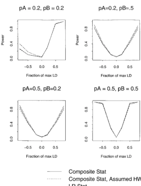
Power:The power of the three statistics is presented (range of simulated values 0.032–0.063, with 2 of 25
falling outside the 95% C.I.; see Figure 3A); the compos- in Figure 4. These simulations assumed HWE, so that all tests could be compared with the same approximate ite statistic with assumed HWE can be grossly
conserva-tive or liberal (range of simulated values 0.006–0.187, type I error rate. Figure 4 illustrates that all three statis-tics have similar power, although there is a small power with 18 of 25 falling outside the 95% C.I.; see Figure
3B); and the likelihood-ratio statistic can have large advantage of the likelihood-ratio statistic when pA1⫽
departures from the nominal 0.05 error rate (range of pB1⫽0.2 and there is negative LD between the loci (see
Figure 2.—Type I error rates based on simulations without LD, but allowing HWD to vary at each locus, in terms offHWD,AandfHWD,B,
the fraction of HWD relative to their extreme values. Two alleles per locus were simulated, with al-lele frequencies pA1⫽pB1⫽0.5.
Figure 3.—Type I error rates for three alleles per locus (equal allele frequencies). Simulations allowed HWD to vary at each lo-cus, in terms offHWD,AandfHWD,Bfor
alleles 1 and 2 at each locus. The types of statistics were: (A) the composite statistic, (B) the com-posite statistic that assumed HWE, and (C) the likelihood-ratio sta-tistic.
assume HWE for the composite statistic and that there Figure 4, left side). Surprisingly, there was no power
difference between the composite test that allowed for can be a significant disadvantage in terms of robustness HWD and that which assumed HWE. These results sug- of the type I error rate to departures from HWE. gest that there is no advantage, in terms of power, to
DISCUSSION
Our simulation results illustrate that when linkage phase is unknown, departures from HWE can have dra-matic effects on the commonly used likelihood-ratio statistic for testing LD. Gross departures from HWE, particularly an excess number of heterozygotes, can in-crease the rate of false-positive conclusions regarding LD. In contrast, the composite statistic provides a robust method to test for LD between loci. This statistic is based on estimates of composite LD and their covariances under the null hypothesis of no LD and no higher-order disequilibria. Our methods are direct extensions of those by Weir and Cockerham, where we derive the covariance between composite measures of LD. An alter-native statistic, proposed by Weir (1979), is based on the goodness-of-fit of the observed phenotype frequen-cies to their null expected values and is implemented in SAS (2003). For large sample sizes, the Wald-type of statistic that we propose and the goodness-of-fit statistic by Weir are expected to give similar results. For sparse data, due to some rare alleles, we speculate that the goodness-of-fit statistic may not be well approximated by the chi-square distribution, as is often found for other goodness-of-fit statistics. Our approach, based on covari-ances of composite LD measures, can use the singular values of the covariance matrix to assess the numerical
Figure 4.—Power for the composite statistic, composite
stability of the statistic and reduce the degrees of
free-statistic that assumed HWE, and likelihood-ratio free-statistic, with
dom according to the rank of the covariance matrix, if
allele frequencies (pA and pB) varied between 0.2 and 0.5.
sample properties of our proposed statistic and the quencies; seeHedrick(1987) for more discussion. Sec-ond, the composite measure depends not only on the goodness-of-fit statistic.
Although it may be tempting to first test for HWE association of alleles between two loci on the same ga-mete (the usualDvalue), but also on the association of and then decide whether or not to assume HWE in the
composite statistic, our simulations suggest that assum- alleles between the two loci on different gametes. This latter type of association is typically ignored, but may ing HWE does not provide any power advantage, yet it
could inflate the type I error rate. This suggests that occur when there are departures from HWE. The com-posite measure of LD is confounded between LD and the composite statistic should be used for routine testing
for LD regardless of whether or not HWE exists at either HWD. Clearly, more work is required to determine the best measure of LD when the assumption of HWE is locus.
Several forces could cause departure from HWE, and violated.
In conclusion, our results suggest that testing for the a critically important cause could be error in the
mea-surement of genotypes. For this reason, departures from presence of LD between two loci with unknown linkage phase should be performed by the composite statistic. HWE are often used as a crude measure of quality
con-trol. This approach, however, does not provide adequate We have extended the work of Weir and Cockerham to allow for more than two alleles at either of the loci, and guidelines on when a marker should be excluded from
the analysis (i.e.,the threshold of statistical significance so this general composite statistic is a strong competitor to the traditional likelihood-ratio statistic.
for concern) or whether particular subjects should be
excluded. An alternative approach is to incorporate ge- This research was supported by United States Public Health Services, notyping errors into methods of analysis, an approach National Institutes of Health, contract grant no. GM65450. that has been successful in linkage analysis of pedigree
data (Sobelet al.2002). Because departures from HWE
could be caused by genotyping errors, explicit models of LITERATURE CITED
genotyping error could be incorporated into the usual
Bailey, N., 1961 Introduction to the Mathematical Theory of Genetic Link-likelihood models for haplotype frequencies, so that age. Oxford University Press, Oxford.
Daly, M., J. Rioux, S. Schaffner, T. HudsonandE. Lander, 2001 departures from HWE would be absorbed into
parame-High-resolution haplotype structure in the human genome. Nat. ters that measure genotyping error rates. More work
Genet.29:229–232.
along this type of modeling may prove beneficial. Al- Devlin, B., andN. Risch, 1995 A comparison of linkage diequili-brium measures for fine-scale mapping. Genomics29:1–12. though our simulations are limited in terms of the many
Excoffier, L., andM. Slatkin, 1995 Maximum-likelihood estima-different patterns of LD that could arise when more
tion of molecular haplotype frequencies in a diploid population. than two alleles exist at either locus, the broad range Mol. Biol. Evol.12:921–927.
Fallin, D., andN. Schork, 2000 Accuracy of haplotype frequency of LD that we explored for the simple case of two alleles
estimation for biallelic loci, via the expectation-maximization al-per locus suggests that the composite statistic has power
gorithm for unphased diploid genotype data. Am. J. Hum. Genet. similar to that of the likelihood-ratio statistic. It may be 67:947–959.
Gabriel, S. B., S. F. Schaffner, H. Nguyen, J. M. Moore, J. Royet al., possible to construct situations where the
likelihood-2002 The structure of haplotype blocks in the human genome. ratio statistic has greater power, yet the potential
infla-Science296:2225–2229.
tion of the type I error rate does not seem to warrant Hawley, M. E., andK. K. Kidd, 1995 HAPLO: a program using the EM algorithm to estimate the frequencies of multi-site haplotypes. routine use of this method.
J. Hered.86:409–411. Our work has focused entirely on determination of
Hedrick, P. W., 1987 Gametic disequilibrium measures: proceed an appropriate way to test for LD, regardless of whether with caution. Genetics117:331–341.
Long, J. C., R. C. WilliamsandM. Urbanek, 1995 An E-M algorithm either locus attains HWE. We have not addressed the
and testing strategy for multiple-locus haplotypes. Am. J. Hum. best way to estimate the amount of LD when there are
Genet.56:799–810.
departures from HWE. Numerous authors have dis- SAS, 2003 Genetics User’s Guide for SAS, Release 8.2 (http://support. sas.com/documentation/onlinedoc/genetics/).
cussed the statistical properties of competing measures
Slatkin, M., andL. Excoffier, 1996 Testing for linkage disequilib-of LD when linkage phase disequilib-of double heterozygotes is
rium in genotypic data using the expectation-maximization
algo-known (Hedrick1987;DevlinandRisch1995;Zabe- rithm. Heredity76:377–383.
Sobel, E., J. C. PappandK. Lange, 2002 Detection and integration
tianet al.2003), but there is little understanding about
of genotyping errors in statistical genetics. Am. J. Hum. Genet. measures of LD when linkage phase is unknown and
70:496–508.
there are departures from HWE. The composite mea- Weir, B., 1979 Inferences about linkage disequilibrium. Biometrics
35:235–254. sure offers appeal, but it can be difficult to interpret
Weir, B., 1996 Genetic Data Analysis II. Sinauer Associates, Sunder-for several reasons. First, it is an additive measure of
land, MA.
the departure of the observed genotype frequency from Weir, B. S., andC. C. Cockerham, 1989 Complete characterization of disequilibrium at two loci, pp. 86–110 inMathematical Evolution-that expected if there were no LD. This is analogous
ary Theory, edited by M. W.Feldman. Princeton University Press,
to the measure D when linkage phase of the double
Princeton, NJ.
heterozygotes is known (i.e.,DAB⫽ pAB⫺pApB). Hence, Zabetian, C. P., S. G. Buxbaum, R. C. Elston, M. D. Kohnke, G. M.
fre-the DBH locus strongly influences fre-the magnitude of association Under this assumption, the probability of the single-between diallelic markers and plasma dopamine beta-hydroxylase
locus genotypeAjAj⬘ is
activity. Am. J. Hum. Genet.72:1389–1400.
Communicating editor: R. W.Doerge P(A
jAj⬘)⫽
兺
k兺
k⬘P(AjBk)P(Aj⬘Bk⬘)
⫽
冢
兺
k
P(AjBk)
冣冢
兺
k⬘P(Aj⬘Bk⬘)
冣
APPENDIX
The random pairing of haplotypes implies that the
⫽ P(Aj)P(Aj⬘),
genotypes at each locus are expected to have genotype proportions in HWE. We can show why this occurs for the case of two loci; it is straightforward to extend our
which illustrates that the probability of the single-locus arguments to more loci. LetAjBkdenote a haplotype. If
genotype is the product of its allele frequencies and haplotypes are randomly paired, the probability of the
hence fits HWE. Symmetric arguments can be used to pair (AjBk,Aj⬘Bk⬘) is
show that single-locus genotypes at theBlocus are also expected to fit HWE.