A Nonlinear Knapsack Problem Arising in Location Problems with Lead Time and Safety Stock Considerations.

(1)

ABSTRACT

JARUGUMILLI, KRISHNA PRASHANT. A Nonlinear Knapsack Problem Arising In Location Problems With Lead Time And Safety Stock Considerations. (Under the direction of Dr. Reha M Uzsoy.)

(2)

c

(3)

A Nonlinear Knapsack Problem Arising In Location Problems With Lead Time And Safety Stock Considerations

by

Krishna Prashant Jarugumilli

A thesis submitted to the Graduate Faculty of North Carolina State University

in partial fulfillment of the requirements for the Degree of

Master of Science

Industrial Engineering

Raleigh, North Carolina

2012

APPROVED BY:

Dr. Brian T Denton Dr. Yahya Fathi

(4)

DEDICATION

This thesis is dedicated in loving memory to S.N.C. Dasaka

(5)

BIOGRAPHY

(6)

ACKNOWLEDGEMENTS

I would like to thank my advisor Dr. Reha M Uzsoy for guiding me and supporting me throughout my research. I thank him for providing me the opportunity to work with him.

I also would like to thank my other committee members Dr. Yahya Fathi and Dr. Brian T Denton for serving in my committee and their valuable comments regarding my thesis.

I would like to thank the entire faculty of Department of Industrial Engineering in North Carolina State University who contributed to my education. I would like to thank my friends in particular: Benjamin Lobo, Nils Buch, Claire Buch, Jennifer Mason, Sean Carr, Hakan Sungur, Hakan Fathi, Peter Prim, Muge Gultekin, Gurdas Sandhu, Ra-jneesh, Erinc Albey, Daniel Underwood, Xi Gong, Yuan Tian; my lab mates(Amirhosein Norouzi, Dr. Yongha Kang, Ilke Bakir, Necip Kacar) in particular for sharing their time and resources. I also thank: Vikram, Nagraj, Kiran, Anand, Narhari, Sandeep, Srikant, Adarsh, Ankur, Balaji, Raveesh, Anup and Suraj for their friendship.

(7)

LIST OF TABLES

Table 2.1 Network design models considering lead time and/or safety stock . 10

Table 3.1 Inputs for the 0-1 knapsack problem . . . 22

Table 3.2 Problem parameters . . . 22

Table 3.3 Illustration of the greedy heuristic . . . 23

Table 4.1 Demand profile for the MPNDLS . . . 31

Table 4.2 Cost Scenarios . . . 31

Table 4.3 Capacity and Relative Priorities . . . 32

Table 4.4 Summary of the experimental design . . . 33

Table 4.5 GA specific factors . . . 34

Table 4.6 Performance of GA and branch-and-bound(BB) algorithm for 15 retailer problem . . . 37

Table 4.7 Computational time of GA for 15 retailer problem(in seconds) . . 37

Table 4.8 % deviation of GA from the linear bound for 49 and 88 retailer problem . . . 45

(9)

LIST OF FIGURES

Figure 1.1 Operations of a DC in the MPNDLS . . . 3

Figure 3.1 Single point and two point crossover(binary encoding) . . . 26

Figure 3.2 Illustration of using random keys for implementing GA . . . 28

Figure 4.1 Average computational time of Branch and bound for 15 node problem . . . 37

Figure 4.2 Objective value of GA(15 retailers) . . . 40

Figure 4.5 Time vs % increase in objective value as a function of population size(49 retailers) . . . 42

Figure 4.6 Time vs % increase in objective value as a function of population size(88 retailers) . . . 43

Figure 4.7 Objective value vs Elitism of GA(88 retailers) . . . 44

(10)

Chapter 1 Introduction

In this chapter, we introduce the Multi Product Network Design Problem and describe the nonlinear 0-1 knapsack problem that is the focus of this thesis, which arises as a subproblem within a Lagrangian heuristic used for the location model. The model we present is that of Sourirajan, Ozsen, and Uzsoy [2011].

1.1 Multi product network design problem

(11)

since the operational effectiveness of a production-distribution network is reflected by the operational performance measures such as customer service level and lead times. In addition, most existing location models consider only a single product. However, different products may have contrasting characteristics(e.g., cost differences), hence aggregating all the different products into a single product may not always be practical.

The work in this thesis arises from an attempt to develop an alternative Lagrangian approach for the multi-product problem that does not require product aggregation. Our work is based on Sourirajan et al. [2011], who consider a two stage supply chain consisting of a set of production facilities and a set of distribution centers. The first stage consists of a set of production facilities that produce different types of products which are shipped to a number of distribution centers at the second stage. Each distribution center(DC), in turn, serves a number of retail demand areas consisting of several independent dealers who serve as the retail outlets. We shall refer to the problem as the Multi-Product Network Design Model considering Lead time and Safety stock, denoted by MPNDLS in the rest of the thesis. We first provide some definitions which we will be using throughout this thesis.

1.1.1 Lead Time

(12)

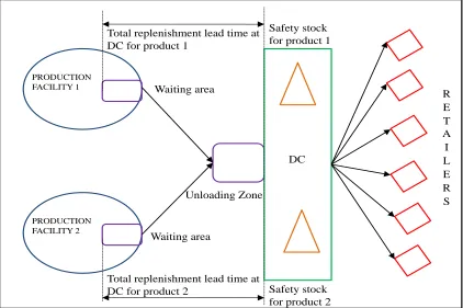
the DCs are sufficiently far from the production facility and that the shipment quantities are sufficiently high so that this approach is valid. When the shipments arrive at the DC, they dock at an unloading zone, where they wait in a First-In-First-Out(FIFO) queue to be unloaded and sent to the retailers. This process is illustrated in Figure 1.1, adapted from Sourirajan, Ozsen, and Uzsoy [2007].

PRODUCTION

FACILITY 1 _{Waiting area}

DC

R E T A I L E R S

PRODUCTION FACILITY 2

Waiting area

Unloading Zone Total replenishment lead time at DC for product 1

Total replenishment lead time at DC for product 2

Safety stock for product 1

Safety stock for product 2

Figure 1.1: Operations of a DC in the MPNDLS

The replenishment lead time for each product at a DC has three components:

1. Load make-up time: This is the queuing time experienced in the outbound

(13)

ordered from a single DC for this product to ensure the shipment of a full truck load of that product to that DC. Consequently, this wait time depends on the demand volume of a product assigned to each DC. As more demand is assigned to the DC, the average load make-up time per unit decreases for that product. Thus, the load make-up time component depends only on the volume of demand of each product assigned to the DC. Note that we assume products cannot share trucks.

2. Constant DC replenishment time (time/unit): This is the replenishment

lead time between the production facility and the DC due to the physical locations of facilities. We assume that it also includes the time spent due to delays such as material handling, general inefficiency and unavoidable processing, such as comple-tion of required paperwork. This component of lead time is not a funccomple-tion of the demand volumes, but of the location of the production facility supplying a given product and the DC receiving the shipment.

3. Congestion time: This is the time spent in the unloading zone of the DC. At high utilization of the unloading resources at the DC, shipments have to wait longer in the queue to be unloaded. This implies that congestion increases as the demand to a location approaches its capacity. Since shipments of all products compete for the same resources at the unloading zone, the total mean demand of all products served by a DC is used in the calculation of expected congestion time.

1.1.2 Service Levels

(14)

high service level and holding cost. In our problem, the DCs carry safety stock to ensure that the retailers achieve their desired service levels. By assigning retailers to a DC, we exploit risk-pooling effects and thus reduce the total inventory held in the system. Eppen [1979] has shown that inventory cost for a centralized system is less than that for a decentralized system. The model we consider uses this result to determine the amount of safety stock to be stored in a DC.

1.2 Research Objective

The objective of MPNDLS is to locate distribution centers to support the operation of a number of retailers by minimizing the sum of fixed facility location costs, transportation costs and inventory holding costs. The problem is formulated as a nonlinear integer programming problem. Solving the nonlinear integer programming problem may be feasible for small problems but as the problem size increases it becomes intractable. Hence by relaxing the assignment constraint, the problem decomposes inton subproblems that have the structure of a nonlinear 0-1 knapsack problem as presented in Sourirajan et al. [2011]. Their Lagrangian heuristic for the multi-product problem uses the procedure developed for the single-product problem by Sourirajan et al. [2007] by aggregating the multiple products into a single product. However, when the products differ widely in their cost structures, this procedure can result in large optimality gaps, although solutions obtained by their genetic algorithm suggest these solutions are likely to be near-optimal. The work we present here arises from an attempt to develop an alternative Lagrangian approach for the multi-product problem that does not require product aggregation.

(15)

branch and bound procedure for this problem to obtain an exact solution. We further use a genetic algorithm and a greedy heuristic to obtain approximate solutions and compare their performance to the solution obtained by branch and bound procedure.

1.3 Complexities of the model

Solving the nonlinear 0-1 knapsack problem is difficult because the objective function is nonlinear and neither convex nor concave. The objective function is also non-separable, which precludes conventional dynamic programming methods(Kellerer et al. [2004]). Due to the nonlinear nature of the problem and the lack of tight lower bounds the branch and bound procedure requires long CPU times. Hence the nonlinearity and the knapsack structure of our problem make it more difficult to solve.

1.4 Thesis Organization

(16)

Chapter 2 Literature Review

In this chapter, we provide the literature review and position our work. We focus on the Multi-product Network design problem and the nonlinear 0-1 knapsack problem. We present a classification of facility location models, discuss the most basic location models such as Uncapacitated Facility Location(UFL), and build up to our network design problem with lead time and safety stock.

Facility location models can be broadly classified based on characteristics such as planning horizon, number of products, distribution of parameters, and the existence of different types of facilities.

1. Planning horizon: If the cost parameters remain unchanged over a long period of time then a single period model is appropriate, whereas, if they may vary over time a multi-period model may be more realistic.

2. Number of products: As the number of products increases, the complexity of

(17)

3. Distribution of parameters: Based on parameters such as demand and lead time, we can classify location models as either deterministic or stochastic.

4. Existence of different types of facilities: A crucial aspect of many practical location problems regards the existence of different types of facilities. The facilities may be identical or may be different with each playing a specific role(i.e., one facility involved in production, while the other may be involved in warehousing).

Francis and Mirchandani [1990], Daskin [1995], and Drezner and Hamacher [2004] discuss facility location problems in great detail. The most basic of all facility location problems is the Uncapacitated Facility Location problem (UFL), in which the objective is to minimize the total cost, made up of facility location costs and transportation costs, subject to demand satisfaction constraints. The problem has been shown to be NP-hard(Krarup and Pruzan [1983]). When a capacity constraint is imposed on UFL, we obtain a Capacitated Facility Location Problem (CFL). Sridharan [1995] reviews the solution methods for CFL. Cornu´ejols et al. [1991], perform a computational study of different relaxations of the CFL. When a constraint of opening only p-facilities is imposed on UFL, we obtain a

P−median problem. These models treat demand arising in different customer locations as deterministic, and focus mainly on the tradeoff between the fixed costs of facility location and variable transportation costs. However, in recent years a number of models have been developed that consider the costs of safety stocks arising from the allocation of customers to service facilities which is the motivation of our study.

(18)

where the lead time to traverse a given distribution center increases nonlinearly with the total flow through the facility due to congestion of resources. Sourirajan et al. [2007] integrates the results of these two streams of research by considering the location of DCs in a two-stage supply chain where lead times at the DCs depend on total flow, and safety stocks take replenishment lead times into account. These authors are able to exploit the structure of the problem to develop an efficient Lagrangian heuristic that yields small optimality gaps. In a subsequent paper, Sourirajan et al. [2011] extend this model to a multiproduct environment. The Lagrangian solution for the single-product problem is used by aggregating the multiple products into a single representative product. However, when products differ widely in their cost structures, this procedure can result in large optimality gaps, although the solutions obtained by a genetic algorithm suggest these solutions are likely to be near-optimal. In this work, we consider an alternative Lagrangian formulation that does not require product aggregation.

(19)

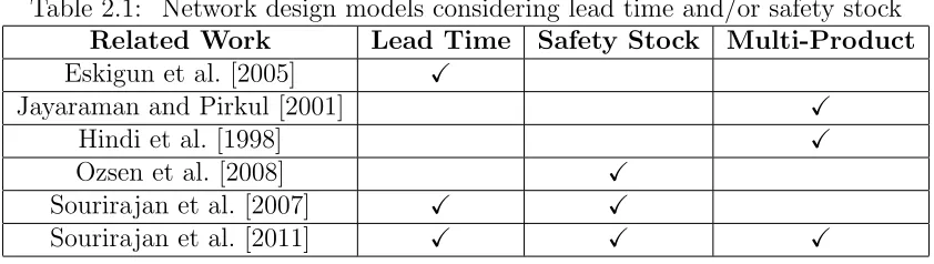
convex nor concave and non-separable. Due to the nonlinear nature of the problem, effi-cient branch and bound procedures are difficult to develop. Hence the nonlinearity and the knapsack structure of our problem make it more difficult to solve than the conven-tional linear 0-1 knapsack problem, which is already NP-hard(Martello and Toth [1990]) in the ordinary sense. In this thesis our focus is on solving the nonlinear 0-1 knapsack subproblem, whose solutions will be later used to develop a Lagrangian procedure for the larger location problems. Table 2.1 gives a summary of the literature on network design problems considering lead time, safety stocks, and number of products.

Table 2.1: Network design models considering lead time and/or safety stock

Related Work Lead Time Safety Stock Multi-Product

Eskigun et al. [2005] _X

Jayaraman and Pirkul [2001] _X

Hindi et al. [1998] _X

Ozsen et al. [2008] _X

Sourirajan et al. [2007] _X _X

(20)

Chapter 3 Modeling and Analysis

In this chapter we discuss the mathematical formulation of the multi-product network design problem considering lead time and safety stock(MPNDLS). The objective of this problem is to minimize the sum of fixed facility location costs, pipeline inventory costs between the production facilities and the distribution centers(DCs) and the cost of safety stocks at the DCs. MPNDLS is subject to set of assignment constraints, linking con-straints, capacity constraints and binary restrictions on decision variables. We wish to develop approximate solutions and lower bounds on the optimal objective function value by relaxing the assignment constraint, yielding subproblems that have the form of 0-1 knapsack problems with a complex, nonlinear objective function.

(21)

are better solution quality and short run time. There is always a trade off between the solution quality and run time. Approximate algorithms that do not guarantee an optimal solution may have significantly smaller run times than branch and bound techniques. Hence, we also present heuristic solution methods including a greedy heuristic and a family of genetic algorithms to obtain approximate solutions and compare them to the optimal solution obtained by branch and bound.

In the rest of the chapter we discuss in detail the mathematical formulation of MP-NDLS and the proposed solution methodologies. Section 3.1 gives a formal statement and formulation of the MPNDLS using Lagrangian multipliers. Section 3.2 presents the nonlinear 0-1 knapsack problem obtained by relaxing the assignment constraint in the original formulation of MPNDLS. In Sections 3.3, 3.4 and 3.5, we discuss the solution methods to the knapsack problem.

3.1 Multi-Product Network Design problem with safety

stock and service level considerations

We consider a Multi-Product Distribution Network Design problem consisting of a set of retailers and distribution centers. Let I be the set of all products, indexed by i =1,...,P and K the set of all retailers, indexed by k=1,...,N. For each product i, a dedicated production facility replenishes retailers located at discrete points within a region where the demand for the product occurs. We aim to locate DCs, each of which serves a set of retailers, such that the sum of the location, pipeline inventory and safety stock costs is minimized.

(22)

stationary Poisson distribution, implying that the variance of the demand is equal to the mean. We also assume that the DCs are close enough to the retailers that pipeline inventory between the retailers and the DCs is negligible. We use the following notation: Parameters

f_j: Fixed cost of locating a DC at candidate site j

C_j: Capacity of the DC at candidate site j

θ_ij: Unit cost of pipeline inventory for producti at DC candidate sitej

H_ij: Unit cost of safety stock inventory for product i at DC candidate site j

p_ij: Load make-up time parameter of lead time at DC candidate sitej for product i q_ij: Constant lead time component per unit at DC candidate sitej for product i

r_j: Congestion parameter of lead time for DC candidate site j

D_ik: Mean demand for product i at retailer k

β_ij: Adjusted safety stock holding cost per unit at DC candidate site j for product i

α_i: Service level that has to be achieved at the retailers for product i

z_α

i: Inverse of the Standard Normal distribution for a probability ofi

Lij: Mean replenishment lead time per unit between the DC candidate site j and the

production facility that produces product i

Zij: Total mean demand of product i assigned to DC j

Decision Variables

y_j =       

(23)

x_ijk =       

1, if demand for product i at retailer k is assigned to DC candidatej 0, otherwise

Before we discuss the mathematical model, we briefly describe the modeling of lead time and service level as presented in Sourirajan, Ozsen, and Uzsoy [2011]. As mentioned in Chapter 1, the replenishment lead time between the DC candidatej and the production facility that serves product i is given by sum of the average load makeup time per unit for producti, the constant DC replenishment time per unit for producti, and the average congestion time per unit for producti as shown in Equation (3.1).

Lij =

pij

Zij

uij +qij+

rjZij

Cj −

P

iZij

(3.1)

From Equation (3.1) it can be seen that the load make up time is nonlinearly decreasing in the demand for a product at a DC, while the congestion time is nonlinearly increasing. This model of lead time is a result of work by Eskigun [2002]. Using Little’s Law, we obtain an expression for the expected pipeline inventory P Iij in the system between the

production facility and the DC given by:

P Iij =LijZij (3.2)

The expected pipeline inventory cost between the production facility serving product i and DC at candidate site j is:

CostP I,ij =θij pijuij +qij

X

k

D_ikx_ijk+ rj P

kDikxijk

C_j −P

l,kDlkxljk

!

(3.3)

(24)

the DC at candidate site j is given by Eppen [1979] as

SSij =zαi

p

LijZij (3.4)

From (3.1) and (3.4), the expected safety stock cost of product i at DC j is given by:

CostSS,ij =Hijzαi

v u u

t p_iju_ij+q_ij X

k

D_ikx_ijk+ rj P

kDikxijk

C_j −P

l,kDlkxljk

!

(3.5)

Using (3.3) and (3.5), we obtain the MPNDLS formulation below:

Minimize X

j

f_jy_j+X

j

X

i:P

kxijk>0

θ_ij p_ij +q_ijX

k

D_ikx_ijk+ rj P

kDikxijk

C_j−P

l,kDlkxljk

! +

X

i:P

kxijk>0

β_ij

v u u

t p_ij +q_ij X

k

D_ikx_ijk+ rj P

kDikxijk

C_j−P

l,kDlkxljk

!

(3.6)

subject to

x_ijk ≤y_j, ∀i, j, k (3.7) X

j

x_ijk = 1, ∀i, k (3.8)

X

i

X

k

D_ikx_ijk ≤C_j, ∀j (3.9)

x_ijk ∈ {0,1}, ∀i, j, k (3.10)

(25)

where β_ij =Hijzαi.

The objective function (3.6) has three terms- the fixed facility location costs, the pipeline inventory costs between the production facilities and the DCs and the safety stock costs at the DCs. Constraint set (3.7) states that we cannot assign demand to location j

unless we locate a DC at j. Constraint set (3.8) is an assignment constraint ensuring that we assign the demand for each product from a particular retailer to exactly one DC. Constraint set (3.9) requires the mean demand flow through a DC to be less than the capacity of a given DC. Constraint sets (3.10)-(3.11) impose binary restrictions on the decision variables.

3.2 Lagrangian Relaxation

(26)

Maxλ∈<Minx,yLD(x, y, λ) =

X

j

f_jy_j +X

j

W_j x₁_j₁· · ·x_{P jN}+X

i,k

λ_ik 1−X

j

x_ijk

!

(3.12) where, W_j x₁_j₁· · ·x_{P jN} is given by

X

i:P

kxijk>0

θ_ij p_ij +q_ijX

k

D_ikx_ijk+ rj P

kDikxijk

C_j −P

l,kDlkxljk

!

+ X

i:P

kxijk>0

β_ij

v u u

t p_ij +q_ij X

k

D_ikx_ijk+ rj P

kDikxijk

C_j−P

l,kDlkxljk

!

(3.13)

Simplifying (3.12), we obtain:

Maxλ∈<Minx,yLD(x, y, λ) =

X

i,k

λ_ik+X

j

f_jy_j −X

i,j,k

λ_ikx_ijk+X

j

W_j x₁_j₁· · ·x_{P jN}

(3.14) subject to

x_ijk ≤y_j, ∀i, j, k (3.15) X

i

X

k

D_ikx_ijk ≤C_j, ∀j (3.16)

(27)

Minimize f_j−X

i

X

k

λ_ikx_ijk+W_j x₁_j₁· · ·x_{P jN}

(3.18)

subject to

X

i

X

k

D_ikx_ijk ≤C_j (3.19)

x_ijk ∈ {0,1} ∀i, k (3.20)

We solve the knapsack problem for location j and based on the objective function value (3.18) we decide if a DC is built at candidate site j i.e., if the objective value is posi-tive then yj=1 else yj=0. Now to consider aforementioned problem as a nonlinear 0-1

knapsack problem, we need to write (3.18) as a maximization problem instead of a min-imization problem, yielding

Maximize −f_j +X

i

X

k

λ_ikx_ijk−W_j x₁_j₁· · ·x_{P jN} (3.21)

(28)

3.3 Branch and Bound Algorithm

The main idea of branch-and-bound is based on an intelligent implicit enumeration of the solution space since in many cases only a small subset of the feasible solutions are enumerated explicitly. It is, however, guaranteed that the parts of the solution space which were not considered explicitly cannot contain the optimal solution. Branch-and-bound algorithms use two main operations, branching and Branch-and-bounding. We now describe these principles.

In the branching operation, a given subset of the solution space X0 ⊆ X is divided into a number of disjoint subsets X1, ..., Xm such thatX1 ∪X2· · · ∪ Xm = X

0

. This process is repeated until either each subset contains only a single feasible solution, or it is determined that it cannot contain the optimal solution z∗. Now by choosing the best solution from all the feasible solutions obtained we can find the optimal solution for the given problem.

The bounding part of a branch and bound algorithm derives upper and lower bounds for a given subset X0 of the solution space. An upper bound zu _≥ _z∗ _{is obtained from}

(29)

The upper bound is usually obtained by relaxation of the original problem. For our nonlinear knapsack problem, we can consider the LP relaxation of the original 0-1 integer problem obtained by ignoring the nonlinear portion. An alternative upper bound on the optimal value of the problem is obtained by establishing an upper bound on the linear term and a lower bound on the nonlinear term of partial unexplored solution. This is done by setting the values of the unexploredxl0s to be one for the linear term and zeros

for the nonlinear term respectively. The upper bound, similar to the lower bound is used to prune parts of the search space. We now present the branch and bound algorithm which is similar to that presented by Kellerer et al. [2004].

Algorithm:

Branch and Bound (l)

l is the index of the next variable to branch on the current solution is x_j =x0_j for j = 1, ..., l−1

q is the value of the nonlinear termW_j x₁_j₁· · ·x_{P jN}, in the objective function 3.21 the current solution subspace is

X0 = (

x_ij ∈ {0,1} |

l−1 X

j=1

w_jx0_j +

n

X

j=l

w_jx_j ≤C

)

if Pl−1

j=1wjx 0

j > c then return

X0 is empty

if Pl−1

j=1pjx 0

j−q > z then

z:=Pl−1

j=1pjx 0

j −q, x∗ :=x 0

improved solution z

if (l > n) then return

X0 contains only the optimal solution derive U

(30)

where Y=nPl−1

j=1λjx 0

j −q+

Pn

j=lλjxj|xj = 1, ∀j =l...n

o

if U

x0 > z then

x0_l= 1, Branch and Bound(l+ 1)

x0_l= 0, Branch and Bound(l+ 1)

3.4 Greedy Heuristic

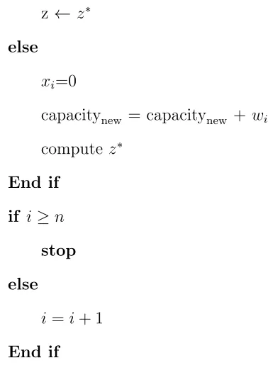
As the name suggests, the principle of the greedy heuristic is to add an item that improves the objective value while satisfying the capacity constraint. Hence at each step, we add an item which increases the objective value the most. The computational complexity of obtaining a solution using a greedy heuristic is low compared to GA or branch and bound. The objective of using the greedy heuristics is to obtain a relatively good feasible solution, which we can use as a lower bound while implementing the branch and bound algorithm. We first give the algorithm for the greedy heuristic, followed by an example where where we illustrate its operation on a two product-three retailer problem(i.e., 6 item knapsack problem).

Inputs w_i, p_i, capacity,n, wherei=1,...,n

Set weight, i,z∗ to 0

Set z to -999

Set capacity_new=capacity

While wi <capacitynew

xi=1

capacity_new = capacity_new -wi

compute z∗

(31)

z ← z∗

else

xi=0

capacity_new = capacity_new +wi

compute z∗

End if

if i≥n

stop

else

i=i+ 1

End if

End while

Following is a specific example that we use to illustrate the application of the greedy heuristic.

Example

Inputs

n= 6, capacity=55

z =−999, i= 1

Table 3.1: Inputs for the 0-1 knapsack problem

Weight 10 12 15 20 25 31

Value 2000 1900 1800 1700 1600 1500

Table 3.2: Problem parameters 1j 2j

pij 1 2

qij 2 4

θij 5 10

(32)

Table 3.3: Illustration of the greedy heuristic Iteration wi capacitynew Feasible z

∗

z Add item

(Capacity (current (current best constraint) objective value) solution value)

1 10 55 Yes 1754 -999 Yes

2 12 45 Yes 3518 1754 Yes

3 15 33 Yes 5128 3518 Yes

4 20 18 No - - No

5 25 18 No - - No

(33)

In this example we implement the greedy heuristic for 2 products and 3 retailers, hence n = 6. Table 3.1 gives the data, value refers to the Lagrangian multipliers and weight

refers to the demand. Table 3.2 gives the values of problem parameters, and the objective value is obtained by substituting the appropriate values in 3.21.

In Table 3.3 we show the iterations of the greedy heuristic. The 2nd_{, 3}rd _{and 4}th

columns of the table give the weight of item i, available capacity before adding item to the knapsack and the feasibility of the capacity constraint. Columns 5 and 6 give the current objective value and current best solution value. Finally column 7 specifies if an item can be added to the knapsack i.e., only if current iteration is feasible and current objective value(z∗) is greater than current best solution value (z).

In Step 6 of the algorithm, at the end of the first iteration we will have only one xijk

equal to 1. As we go through more iterations we add more items to the knapsack as long as the objective function value is non-decreasing. In the process of implementing this algorithm, we may obtain a solution where we might add one item in the first iteration and fail to add further items. This situation will arise when all the items considered in the subsequent iterations decrease the total objective value. To obtain an approximate solution to the nonlinear 0-1 knapsack problem we have embedded the Greedy heuristic with our Genetic Algorithm described in the next section.

3.5 Genetic Algorithm

(34)

be specified for any given implementation are representation, population, evaluation, selection, operators and parameters. In this thesis we use a GA to obtain approximate solutions for the nonlinear knapsack problems which are the focus of this research. In this section we give definitions of the basic elements and a brief outline of the operation of GA.

1. Chromosomes: The strings or chromosomes that represent a solution to the prob-lem being studied are the building blocks of GAs. A set of these chromosomes is called a population.

2. Reproduction: Individual solutions are selected from the current population

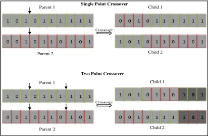
based on their fitness function values and new solutions(offspring) generated by combining and modifying the genes of these solutions. Selection of the parent strings may be biased in favor of solutions with better fitness values. Crossover and mutation are the main mechanisms for driving the reproduction process among chromosomes. Crossover combines the genes of two parents to produce offspring, while mutation randomly alters individual genes to ensure diversity of solutions. Figure (3.1) illustrates single point and two point crossover mechanisms. In our GA implementation, we use random keys to represent a solution, hence our crossover mechanism is somewhat different, as will be discussed later in this Chapter.

(35)

1 0 1 0 1 1 1 1 1 1

0 0 1 0 1 1 0 1 0 1 0 0 1 0 1 1 1 1 1 1

1 0 1 0 1 1 0 1 0 1

Parent 1

Parent 2

Crossover

Child 1

Child 2

1 0 1

1 1 1

1 0 1 0 1 1 1 1 1 1

0 0 1 0 1 1 0 1 0 1

0 1 1 1 1 1 1

0 0 1

1 0 1 0 1 1 0 1 0 1

Parent 1

Parent 2

Crossover

Child 1

Child 2 Single Point Crossover

Two Point Crossover

Figure 3.1: Single point and two point crossover(binary encoding)

generated independently of previous solutions.

Another mechanism we employ is an elitist strategy, the direct transfer of solutions with high fitness values to the next population to ensure that the value of the best solution encountered so far is monotonically non-decreasing from one generation to the next (for a maximization problem). Population convergence to a local maxi-mum is a potential downside of this strategy. Hence it must be accompanied by a suitable diversification strategy such as mutation or immigration.

(36)

con-sider the ranking method. In this method, we rank the chromosomes based on their objective value. Each of the chromosomes is assigned a relative probability,

Pi = f fi/

P

if fi, where Pi is the relative probability of selection of the i

th

chro-mosome; f fi is the fitness(objective) function value of the ith chromosome. From

these relative probabilities we compute the cumulative probabilities. Now using a pseudo random number generator, generating numbers between 0 and 1, we can select the chromosomes for crossover such that those with higher fitness value have higher probability of selection.

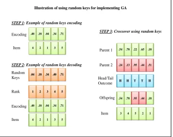
4. Coding schemes: The different coding schemes for representing a solution are: binary coding, integer coding, real number coding, and other specially designed codings. The binary coding scheme can be easily implemented for our problem i.e., 1 represents that we have the item in the knapsack while 0 represents we don’t add the item. However, the binary encoding does not allow us to distinguish between feasible and infeasible solutions. To overcome this disadvantage of binary encoding, we use the random keys approach (Bean [1994]) which eliminates the issue of infeasible chromosomes. We now give the procedure for implementing genetic algorithms using random keys.

(a) Generate n random variates between 0-1 for the x vector(i.e., for product of number of products and retailers). In case of 49 retailer(k) problem and 2 products(i), there will be 98(n) such random variates.

(b) Sort the random variates in ascending order.

(c) Set the iterator j to 0.

(37)

.54 Parent 1

STEP 3: Crossover using random keys

.78 .22 .65 .18

.24 .13 .95 .44 .51 Parent 2

H H T T H Head/Tail

Outcome

Offspring .54 .78 .95 .44 .18 .18 .40

Encoding .18 .04 .34 .71

4 2 1 3 5 Item

STEP 1: Example of random keys encoding

.40

Encoding .18 .04 .34 .71

4 2 1 3 5 Item

.04 Random

Keys .18 .34 .40 .71

1 2 3 4 5 Rank

STEP 2: Example of random keys decoding

3 4 5 2 1 Item

Illustration of using random keys for implementing GA

Figure 3.2: Illustration of using random keys for implementing GA

(e) If capacity constraint is violated in step d remove the jth _{item from knapsack}

and update capacity, else continue tostep f.

(f) If j ≥n continue tostep g, else j =j+ 1 and gotostep d. (g) Repeat steps a tof for all chromosomes in the population.

(38)

(39)

Chapter 4 Experimental Design and Results

In this chapter we present the design of our computational experiments and provide the computational results and analysis for various test instances.

4.1 Design of Experiments

We test our algorithms on six different instance sizes defined by the number of nodes and number of products. Each node represents a retailer location, and all retailer locations are candidates for locating DCs.

(40)

the variance of demand will be equal to the mean demand.

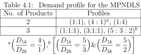
Table 4.1: Demand profile for the MPNDLS No. of Products Profiles

2 (1:1), (4 : 1)a, (1:4) 3 (1:1:1), (3:1:1), (5 : 3 : 2)b aD1k

D2k

= 4 1

,b

D₁_k

D2k

= 5 3

&

D₁_k

D3k

= 5 2

For both the two and three product problems, the ratios are used as a baseline around which we generate the individual product demands for a retailer. We randomly pick the demand profiles for each retailer from the three profiles given in Table 4.1 and ensure that the number of retailers with a given demand profile is approximately the same. We also consider cost scenarios with equal and unequal costs across products using the cost ratios in Table 4.2. For simplicity we refer to cost scenarios with equal and unequal costs across products as no cost difference(ncd) and cost difference(cd), respectively.

Table 4.2: Cost Scenarios No. of Products Profiles

2 (1:1), (1 : 2)a

3 (1:1:1), (1/5 : 1 : 5)b aθ1j

θ2j

= β1j

β2j

= 1 2

,b

θ₁_j

θ2j

= β1j

β2j

= 1 5

&θ1j

θ3j

= β1j

β3j

= 1 25

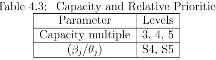
For each cost scenario, we explore the sensitivity of the solution to different weights on pipeline inventory and safety stock (Table 4.3). As we go from S4 to S5, the ratio of the safety stock cost to pipeline inventory cost in the objective function for each product increases by a factor of 10(S4=1000, S5=10000).

(41)

Table 4.3: Capacity and Relative Priorities Parameter Levels

Capacity multiple 3, 4, 5 (βj/θj) S4, S5

capacity multiple increases, the total available system capacity increases. We also vary the priority given to safety stocks over the pipeline inventory costs as given in Table 4.3. We consider only two levels of safety stock factor because the effect of safety stock factor at lower levels was negligible in our pilot experiment. Since we assume Poisson demand at the retailers, variances are set equal to the mean demand values. We use

zα=2.00, corresponding to a 97.75% service level. The constant DC replenishment lead

timeqij is arbitrarily set to ten for all candidate locationsj and we use the values forpij,

rj, and Cj proposed by Sourirajan et al. [2007](refer to the Appendix for derivation of

parameters). A challenging aspect of this problem is the determination of values to the coefficients of the linear component of the objective function. In the Lagrangian scheme that is our ultimate objective, these coefficients will be determined by the values of the Lagrange multipliers at each iteration. However, without solving the Lagrangian problem it is difficult to estimate a range for these coefficient values. In this thesis we take the approach of generating these coefficients as a function of the demand associated with the customer site, computed by multiplying the mean demand at the site by a uniform random variate between zero and 10.

(42)

ncd respectively.

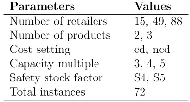
Table 4.4: Summary of the experimental design

Parameters Values

Number of retailers 15, 49, 88 Number of products 2, 3 Cost setting cd, ncd Capacity multiple 3, 4, 5 Safety stock factor S4, S5 Total instances 72

Table 4.5 summarizes the experimental design for genetic algorithm. We performed 5 replications for each problem instance. For the 15 node problems we considered only one level of the factors population and stopping criteria, since we computed the optimal solution using branch and bound algorithm. For 49 node and 88 node problems we considered all levels as given in Table 4.5, and obtained a simple upper bound by taking the LP relaxation of nonlinear 0-1 knapsack problem ignoring theWj term in 3.21. Since

the appropriate values of population and stopping criteria in the GA are likely to depend on problem size, we relate them to the number of retailers. We terminate the procedure when the best solution found has not improved in 2n generations for 15 retailer problem,

(43)

Table 4.5: GA specific factors Parameter Levels Population size 3n, 5n, 10n

Stopping criteria 3n, 5n, 10n

Elite factor .05, .1, .15 Immigration factor .05, .1, .15

4.1.1 Algorithm-Related Factors

In the previous section we discussed the factors specific to the model formulation given in Table 4.1, 4.2 and 4.3. In this subsection, we list the factors we consider for the experiment specific to genetic algorithm (refer Table 4.5). We give a brief description of each of the factors that include population size, stopping condition, and crossover rate.

(44)

2. Reproductive strategy(Crossover/Immigration/Elitism): We consider all the three terms together since Pcrossover +Pimmigration +Pelitism = 1. Elitism is

selecting the best solutions of the current generation and passing them to the next generation. We use the overlapping population criterion by passing a fraction of the best solutions of the current generation to the next generation. Immigration is the random generation of new chromosomes as part of the diversification process. Crossover combines the genes of two parents to produce offspring. In our experi-ment we have considered three levels of immigration and elitism, keeping crossover constant(refer Figure (3.1)). By varying these two factors we can control the diver-sification and intendiver-sification process. We investigate the influence of these factors for finding the final solution.

3. Stopping Criteria: The stopping criteria is a significant factor for any genetic algorithm. We use a flexible stopping criteria described below.

if zx−zx−1 > then

k =x+i.n

end

where,

zx: Objective value in generation x

zx−1: Objective value in generation x-1

: significant difference from generationx-1 to generation x(In our problem = 0)

i: multiple of Stopping criteria(1, 3 and 5)

n: product of number of retailers and number of products

(45)

In the flexible stopping criteria, we compute the difference in the objective function values of best solutions in generation x and x−1. If the increase in objective function value is significant,i.e., greater than then we increase the minimum number of generations before we terminate the search by a factor.

4.2 Computational results

In this section, we present the numerical study and compare the performance of branch and bound algorithm and the GA. We compare the GA solution to the optimal solution obtained by the branch and bound algorithm for 15 retailer problems, while for the 49 and 88 retailer problems we use an upper bound obtained from LP relaxation by ignoring the nonlinear term in 3.21, i.e., 0 ≤ xijk ≤ 1. Table 4.6 illustrates the computation

time for the branch and bound algorithm(4th _{column), which increases exponentially}

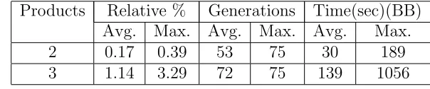
with the increase in number of products for 15 retailer problem(refer Figure 4.2). The capacity multiplier also has a major effect on the computational time. When the capacity increases, we allow more items to be added to the knapsack, which further increases the number of nodes to be explored resulting in an increase in computational time. We also give the relative performance(2nd column) of the GA to the optimal solution and the number of generations(3rd column) for GA to terminate. We see in Table 4.7 that on average the GA yields solutions which are within 2% of the optimal solution in only a few seconds of computation time.

(46)

Table 4.6: Performance of GA and branch-and-bound(BB) algorithm for 15 retailer problem

Products Relative % Generations Time(sec)(BB) Avg. Max. Avg. Max. Avg. Max.

2 0.17 0.39 53 75 30 189

3 1.14 3.29 72 75 139 1056

Table 4.7: Computational time of GA for 15 retailer problem(in seconds) No. of items Capacity multiple No Cost difference Cost difference

(ncd) (cd)

Avg SD Avg SD

30

3 0.45 0.09 0.45 0.08

4 0.51 0.14 0.52 0.08

5 0.60 0.15 0.57 0.10

45

3 1.36 0.28 1.40 0.29

4 1.64 0.26 1.73 0.32

5 1.79 0.27 1.92 0.36

0 50 100 150 200 250 300 350

S4 S5 S4 S5 s4 s5 s4 s5

ss factor ss factor ss factor ss factor

ncd cd ncd cd

2 products 3 products

T

im

e(sec)

Capacity multiple 3

Capacity multiple 4

Capacity multiple 5

(47)

For a fixed relative priority between safety stock and pipeline inventory as the capacity level increases the objective function value increases, which is intuitive. We also see a decreasing trend in objective value as the relative priority factor increases, due to the increase in the nonlinear term at each level. We also see a decreasing trend in the objective value as the number of products increases, because the objective value is a function of capacity which is dependent on the mean demand(i.e., mean demand for three products is less than two products).

(48)

this section, increasing capacity increases the number of items added to the knapsack resulting in more iterations. Increasing the population size, increases the computational complexity of computing objective value for all chromosomes in each generation and also increases the complexity in the ranking process.

Hence, we observed that the problem parameters that affected the computational time of GA are capacity multiple, number of products, cost difference and the safety stock factor. The GA factors that affected the time and solution quality are population size and stopping criterion. The other factors: immigration and elitism didn’t have significant effect on the solution quality.

(49)

2.00E+08 2.50E+08 3.00E+08 3.50E+08 4.00E+08 4.50E+08

S4 S5 S4 S5 S4 S5 S4 S5

cd ncd cd ncd

Ob jectiv e f u n ctio n v alu e

Capacity multiple 3 Capacity multiple 4 Capacity multiple 5

Figure 4.2: Objective value of GA(15 retailers)

4.00E+08 5.00E+08 6.00E+08 7.00E+08 8.00E+08 9.00E+08 1.00E+09 1.10E+09 1.20E+09

S4 S5 S4 S5 S4 S5 S4 S5

cd ncd cd ncd

Ob jectiv e f u n ctio n v alu e

Capacity multiple 3

Capacity multiple 4

Capacity multiple 5

(50)

0.00E+00 5.00E+07 1.00E+08 1.50E+08 2.00E+08 2.50E+08

S4 S5 S4 S5 S4 S5 S4 S5

cd ncd cd ncd

Ob

jectiv

e f

u

n

ctio

n

v

alu

e

Capacity multiple 3

Capacity multiple 4

Capacity multiple 5

(51)

n 3n 5n

3n 5n 3n

5n

n

5n

3n

0 20 40 60 80 100 120 140 160 180 200

0.00 0.20 0.40 0.60 0.80 1.00 1.20

T

im

e

(sec)

% increase in objective value

98 items ncd

98 items cd

147 items ncd 147 items cd

(52)

3n

5n 3n

5n n

3n 5n

0 200 400 600 800 1000 1200

0.00 0.10 0.20 0.30 0.40 0.50 0.60

T

im

e

(sec)

% increase in objective value

176 items ncd

176 items cd

264 items ncd 264 items cd

(53)

0.00E+00 5.00E+07 1.00E+08 1.50E+08 2.00E+08 2.50E+08

0.05 0.1 0.15

Elitism

Object

ive

function va

lue

Capacity 3 Capacity 4 Capacity 5

Figure 4.7: Objective value vs Elitism of GA(88 retailers)

0.00E+00 5.00E+07 1.00E+08 1.50E+08 2.00E+08 2.50E+08

0.05 0.1 0.15

Immigration

Object

ive

function va

lue

Capacity 3 Capacity 4 Capacity 5

(54)

Table 4.8: % deviation of GA from the linear bound for 49 and 88 retailer problem No. of retailers No. of products Capacity Multiple SS factor

S4 S5

Avg (%) Min (%) Max (%) Avg (%) Min (%) Max (%)

49

2

3 8.24 8.20 11.49 10.34 10.29 12.82

4 7.36 7.30 8.96 9.69 9.52 12.15

5 6.18 6.13 7.52 8.34 8.32 9.90

3

3 6.50 5.10 8.23 7.55 6.94 8.35

4 5.94 4.51 18.73 6.75 5.57 8.98

5 4.28 3.26 15.73 4.05 3.66 4.72

88

2

3 8.81 8.74 9.29 13.55 13.45 14.15

4 7.82 7.52 8.44 12.20 12.01 12.85

5 7.09 6.84 7.79 11.16 10.74 12.71

3

3 3.32 2.97 4.20 10.35 9.94 11.84

4 2.87 2.64 3.86 9.04 8.75 10.00

(55)

Table 4.9: Computational time of GA for 49 and 88 retailer problems(in seconds)

No. of items Capacity multiple No Cost difference (ncd) Cost difference (cd)

n 3n 5n n 3n 5n

Avg SD Avg SD Avg SD Avg SD Avg SD Avg SD

98

3 2.3 1.2 11.2 6.1 24.8 13.0 2.6 1.3 12.7 6.9 27.7 14.5

4 2.5 1.3 12.0 6.4 25.8 13.5 2.8 1.4 12.9 6.8 28.4 14.7

5 2.8 1.5 12.4 6.5 27.2 13.4 3.0 1.5 13.6 6.8 29.5 14.7

147

3 17.5 12.0 81.4 64.2 176.2 107.6 21.2 10.0 137.6 71.2 121.3 59.9 4 21.4 13.8 94.8 64.6 190.2 112.8 23.4 10.8 175.9 90.9 137.7 67.6 5 20.1 14.7 87.2 55.2 194.6 112.3 25.5 12.0 220.4 120.0 153.4 75.7

176

3 18.2 10.0 134.6 71.2 118.3 59.9 17.8 9.9 149.6 75.2 130.1 70.0 4 20.4 10.8 172.9 90.9 134.7 67.6 19.3 10.5 158.6 82.8 143.5 72.4 5 22.5 12.0 217.4 120.0 150.4 75.7 21.4 11.4 226.4 128.1 150.8 74.3

264

(56)

Table 4.10: Objective function value obtained by GA(in 105₎

# of items CM No Cost difference (ncd) Cost difference (cd)

S4 S5 S4 S5

Avg SD Avg SD Avg SD Avg SD

30

3 2852.91 2.04 2743.44 17.82 2841.53 9.29 2685.63 16.71 4 3703.50 6.01 3584.79 10.72 3696.94 3.61 3522.29 14.55 5 4540.41 16.28 4386.79 21.59 4522.44 25.87 4326.16 10.20

45

3 2658.55 33.95 2548.11 19.13 2588.37 57.77 2308.83 25.50 4 3328.58 27.58 3145.43 62.48 3269.54 17.60 2891.94 41.81 5 3879.34 24.42 3664.51 155.53 3781.35 127.68 3413.92 54.85

98

3 6736.71 48.64 6573.69 52.31 6721.61 70.05 6566.87 65.86 4 9045.44 43.24 8819.11 38.59 9006.15 53.43 8786.07 91.31 5 11391.30 57.39 11117.11 53.74 11358.67 50.72 11111.23 57.39

147

3 4159.19 17.38 4123.69 13.67 4418.98 830.36 4125.91 19.13 4 5635.99 32.13 5515.98 30.88 5501.48 432.40 5526.42 48.34 5 7129.10 14.34 7070.62 8.64 6984.39 458.94 7076.73 16.80

176

3 1443.96 2.79 1371.50 4.59 1430.93 1.24 1354.13 1.28 4 1935.49 7.61 1841.99 7.53 1914.71 3.84 1825.39 2.54 5 2421.45 7.81 2320.71 16.13 2404.07 6.79 2293.07 7.89

264

(57)

Chapter 5 Conclusions and Future Work

In this thesis, we introduced the Multi Product Network Design Problem developed by Sourirajan et al. [2011] that considers lead times and safety stocks to improve the operational efficiency of a production-distribution system.

In Chapter 1, we introduced the MPNDLS problem. We noted that most models in facility location and allocation models focus on tradeoff between the fixed costs of facility location on the one hand, and the variable cost of transportation on the other. Also, our model incorporates lead times and the cost of safety stocks arising from the customers to service facilities. The lead time we consider consists of three components: load makeup time, constant DC replenishment time and congestion time. Load makeup time is observed at the production facility while waiting for sufficient demand to be ordered from a single DC. Constant DC replenishment time is the replenishment lead time between the production facility and the DC due to the physical locations of the facilities. Finally, the congestion time is the time spent in the unloading zone. We also consider safety stocks for the DC for the retailers to achieve their desired service levels.

(58)

problems. We broadly classified the facility location models in four categories based on planning horizon, number of periods, distribution of parameters, and existence of different types of facilities. We also discussed various facility location problems such as the Uncapacitated Facility Location problem(UFL), Capacitated Facility Location problem (CFL) and P-median problem. We emphasized the significance of lead times, safety stocks and multiple products begin considered together for the model to reflect the real world scenario. We also noted that the Lagrangian approach proposed in this thesis doesn’t require product aggregation. We also provided literature review on the knapsack problems

In Chapter 3, we presented the mathematical model for the MPNDLS developed by Sourirajan et al. [2011]. We then relaxed MPNDLS to obtain n 0-1 nonlinear knapsack subproblems, which form the subject of this thesis. The complex nonlinear, neither convex nor concave and non-separable structure of the knapsack problem prevent the use of conventional dynamic programming techniques. Hence to solve the problem optimally we developed a branch and bound algorithm. We also developed a greedy heuristic which we embedded within our GA to obtain approximate solutions for larger nonlinear knapsack problems. We could solve only 15 retailer problems (30 and 45 item) with branch and bound, and for 49 retailer (98 items and 147 items) and 88 retailer (176 items and 264 items) we obtained approximate solutions using the GA. We also described in detail the chromosome representation, various reproduction strategies(elitism, crossover and immigration) and selection mechanism.

(59)

to the knapsack, which increases the number of nodes explored. The objective function value also increased with the capacity multiple, and decreased with increase in safety stock cost factor. We also observed that the genetic algorithm gave good solutions with reasonable computational time. In the case of GA too, we observed that as the capacity multiple and population size increased the computational time of GA increased. We observed that the quality of solutions obtained by GA improved as we allowed the GA to run for longer durations. In our problem time is a function of population size and stopping criterion. At high levels of population size and stopping criterion we obtained good quality solutions. For the 15 retailer problems we compared the solutions obtained by GA to the optimal solutions obtained by branch and bound. We obtained solutions within 2% of optimality on average. For the larger 49 and 88 retailer problems we compared the solution obtained by GA to upper bounds obtained from LP relaxation by ignoring the nonlinear term in objective function. We observed that the solutions obtained GA were within 12% of upper bounds.

(60)

REFERENCES

J.C. Bean. Genetic algorithms and random keys for sequencing and optimization. ORSA Journal on Computing, 6(2):154–160, 1994.

K.M. Bretthauer and B. Shetty. The nonlinear knapsack problem-algorithms and ap-plications. European Journal of Operational Research, 138(3):459–472, 2002. ISSN 0377-2217.

G. Cornu´ejols, R. Sridharan, and J.M. Thizy. A comparison of heuristics and relaxations for the capacitated plant location problem. European Journal of Operational Research, 50(3):280–297, 1991. ISSN 0377-2217.

M. S. Daskin. Network and Discrete Location: Models, Algorithms and Applications. John Wiley and Sons, Inc., New York, 1995.

Z. Drezner and H.W. Hamacher. Facility location: applications and theory. Springer Verlag, 2004. ISBN 3540213457.

G.D. Eppen. Effects of centralization on expected costs in a multi-location newsboy problem. Management Science, 25(5):498–501, 1979. ISSN 0025-1909.

E. Eskigun. Outbound supply chain network design for a large-scale automotive company. ETD Collection for Purdue University, 2002.

E. Eskigun, R. Uzsoy, P.V. Preckel, G. Beaujon, S. Krishnan, and J.D. Tew. Outbound supply chain network design with mode selection, lead times and capacitated vehicle distribution centers. European Journal of Operational Research, 165(1):182–206, 2005. M.L. Fisher. The lagrangian relaxation method for solving integer programming

prob-lems. Management science, pages 1–18, 1981.

R.L. Francis and P.B. Mirchandani. Discrete location theory. Wiley, 1990.

M.R. Garey and D.S. Johnson. Computers and Intractability: A Guide to the Theory of NP-completeness. WH Freeman & Co. New York, NY, USA, 1979. ISBN 0716710447. D.E. Goldberg. Genetic algorithms in search, optimization, and machine learning.

Addison-wesley, 1989. ISBN 0201157675.

(61)

S. Huang, R. Batta, and R. Nagi. Distribution network design: selection and sizing of congested connections. Naval Research Logistics, 52(8):701–712, 2005.

V. Jayaraman and H. Pirkul. Planning and coordination of production and distribution facilities for multiple commodities. European Journal of Operational Research, 133(2): 394–408, 2001.

H. Kellerer, U. Pferschy, and D. Pisinger. Knapsack problems. Springer Verlag, 2004. J. Krarup and P.M. Pruzan. The simple plant location problem: Survey and synthesis.

European Journal of Operational Research, 12(1):36–81, 1983.

Fernando Lobo and Cludio Lima. Adaptive population sizing schemes in genetic al-gorithms. In Fernando Lobo, Cludio Lima, and Zbigniew Michalewicz, editors, Pa-rameter Setting in Evolutionary Algorithms, volume 54 of Studies in Computational Intelligence, pages 185–204. Springer Berlin / Heidelberg, 2007.

S. Martello and P. Toth. Knapsack problems: algorithms and computer implementations. 1990.

L. Ozsen, C.R. Coullard, and M.S. Daskin. Capacitated warehouse location model with risk pooling. Naval Research Logistics, 55(4):295–312, 2008.

K. Sourirajan, L. Ozsen, and R. Uzsoy. A single-product network design model with lead time and safety stock considerations. IIE Transactions, 39(5):411–424, 2007.

K. Sourirajan, L. Ozsen, and R. Uzsoy. An Integrated Multi-product network design model with lead time and safety stock considerations.Research Report, Edward P. Fitts Department of Industrial and Systems Engineering, North Carolina State University, 2011.

R. Sridharan. The capacitated plant location problem. European Journal of Operational Research, 87(2):203–213, 1995. ISSN 0377-2217.

(62)

(63)

Appendix A

Appendix

The following discussion on derivation of problem parameters is adopted from Sourirajan et al. [2007].

The lead time expression used in this thesis is motivated by the results of an extensive simulation study in the automotive industry Eskigun [2002]. However, to test our model, we need to determine reasonable lead time parameters. For this, we use the queueing-analysis-based method outlined in this section to get reasonable values for the lead time parameters. We continue to user as the congestion parameter andpas the load make-up time parameters in our models to maintain a general lead time expression as we can use any reasonable value ofr without changing the results and the solution procedure. Given that we assume the retailer demand process to be Poisson, the demand process at the DC, obtained by a super-position of the retailer demands, is also Poisson.

Load make-up time

(64)

is sent to the DC. Given that the demand process is Poisson at the DCs, let the mean inter arrival times between the product arrivals from the production facility be µ. Let the truck capacity be M products. Since the production facility sends full truckloads to the DCs, the products arriving at the waiting area of the production facility wait till a batch equal to the truck capacity accumulates. Using standard queueing, we have that the Mth product to arrive in a batch does not have to wait to be sent to the DC, the (M - 1)st product has to wait for µtime units on an average and so on. Let LMU(k) be the average time the kth product has to wait. We have LMU(k) = (M−k)µ. Thus, the load make-up time, LM Uavg, which gives the average time a product has to wait at the

production facility is derived as below:

LM Uavg =

PM

k=1LM U(k)

M =

PM

k=1(M −k)µ

M

= M(M −1)/2

M µ=

(M −1)/2

Z

where Z is the total mean demand assignment to the DC. In this thesis, we use the expression for load make-up time to be of the form (p/Z), where p is the load make-up time parameter. Thus, as we can see from the above derivation, p = (M - 1)/2.

Congestion time

(65)

average number of trucks that can be processed by the DC per period. We further assume that the unloading docks have separate queues and the truckload arrivals are split equally between the queues. Thus, an unloading dock faces a mean arrival rate of

Z/M C/M

=

Z C

and has a mean processing rate of one truck load per time period. Assuming each unloading dock is an M/M/1 system, the average time in system per unit, TIS, which gives the congestion time per unit can be written as

Congestion time = 1

(1−(Z −C)) =

C C−Z