DOI: 10.1534/genetics.107.080838
Accuracy of Genomic Selection Using Different Methods to
Define Haplotypes
M. P. L. Calus,*
,1T. H. E. Meuwissen,
†A. P. W. de Roos
‡and R. F. Veerkamp*
*Animal Breeding and Genomics Centre, Animal Sciences Group, Wageningen University and Research Centre, 8200 AB Lelystad, The Netherlands,†University of Life Sciences, Department of Animal and Aquacultural Sciences, N-1432 A˚ s, Norway and
‡HG, 6802 EB Arnhem, The Netherlands
Manuscript received August 20, 2007 Accepted for publication November 6, 2007
ABSTRACT
Genomic selection uses total breeding values for juvenile animals, predicted from a large number of estimated marker haplotype effects across the whole genome. In this study the accuracy of predicting breeding values is compared for four different models including a large number of markers, at different marker densities for traits with heritabilities of 50 and 10%. The models estimated the effect of (1) each single-marker allele ½single-nucleotide polymorphism (SNP)1, (2) haplotypes constructed from two adjacent marker alleles (SNP2), and (3) haplotypes constructed from 2 or 10 markers, including the covariance between haplotypes by combining linkage disequilibrium and linkage analysis (HAP_IBD2 and HAP_IBD10). Between 119 and 2343 polymorphic SNPs were simulated on a 3-M genome. For the trait with a heritability of 10%, the differences between models were small and none of them yielded the highest accuracies across all marker densities. For the trait with a heritability of 50%, the HAP_IBD10 model yielded the highest accuracies of estimated total breeding values for juvenile and phenotyped animals at all marker densities. It was concluded that genomic selection is considerably more accurate than traditional selection, especially for a low-heritability trait.
T
HE availability of many thousands ofsingle-nucleotide polymorphisms (SNPs) spread across the genome for different livestock species opens up possibilities to include genomewide marker informa-tion in predicinforma-tion of total breeding values, to perform genomic selection. Compared to traditional breeding practice, including genomic information yields a consid-erable increase in selection responses for juvenile ani-mals that do not have phenotypic records (Meuwissen
et al. 2001) and potentially can reduce the costs of a breeding program up to 90% (Schaeffer2006).
Genomic selection as described by Meuwissen et al.
(2001) predicts total breeding values on the basis of a large number of marker haplotypes across the entire genome. The underlying assumption of genomic selec-tion is that haplotypes at some loci are in linkage dis-equilibrium (LD) with QTL alleles that affect the traits that are subject to selection. Different ways of deriving haplotypes of combinations of marker alleles, and the relationship between haplotypes at a locus, have been described. One method (SNP1) is to consider each different marker allele at a single locus to be a different haplotype, considering no relationships between differ-ent haplotypes, and thus breeding values are estimated
directly for the marker alleles (Xu 2003). A second
method is to construct haplotypes from two alleles at adjacent markers, assuming a zero relation between haplotypes at the same locus (SNP2) (Meuwissenet al.
2001). A third method is to construct haplotypes (HAP_IBD) using two or more surrounding marker alleles and derive identical-by-descent (IBD) probabili-ties between the different haplotypes at the same locus (Meuwissenand Goddard2001).
The SNP1 model considers only two haplotypes at a locus and therefore may be suited for applications in, for instance, double-haploid populations with only two segregating genotypes at each locus (Xu 2003). For
outbred populations, where the association between markers and QTL might be different in different fam-ilies, the SNP1 model is perhaps less well suited. The advantage of the SNP1 approach is that determining the linkage phase of the haplotypes is not required and the markers do not need to be mapped. A disadvantage of the SNP1 model is that no new haplotypes arise as a result of recombination, while such an event actually might change the linkage between the marker and the QTL alleles. SNP1 and SNP2 do not make a distinction between haplotypes that are alike-in-state (AIS) due to a common ancestor (i.e., IBD) or simply due to chance. The benefit from the HAP_IBD approach is that the common background of haplotypes, and thus the prob-ability that different haplotypes are associated with the
1Corresponding author:Animal Breeding and Genomics Centre, Animal
Sciences Group, Wageningen University and Research Centre, P.O. Box 65, 8200 AB Lelystad, The Netherlands. E-mail: [email protected]
same QTL allele, is modeled more accurately. The HAP_IBD approach, as well as SNP2, however, does require an accurate marker map and the determination of the linkage phase. A disadvantage of the HAP_IBD approach is that it likely will yield much more effects at a single locus that need to be estimated.
The three different approaches have been compared before for their ability to fine map a single QTL (Grapes
et al. 2004). Although it was shown that the SNP1 method was able to compete with the HAP_IBD method, the HAP_IBD method gave more accurate results at the same number of markers (Grapeset al.2004). Arguably,
genomewide selection could be seen as a special appli-cation of multiple-QTL fine mapping. The main differ-ence is that QTL fine mapping aims at determining the position of the QTL, whereas in genomewide selection the aim is to predict accurate breeding values.
The objective of this study was to compare the accu-racy of predicted breeding values used in genomic selection for an outbred population with these three different ways of including genomewide marker in-formation. Since it is expected that the difference in marker density is an important factor, these methods are compared at five marker densities ranging from 1 marker/0.13 cM to 1 marker/2.52 cM.
MATERIALS AND METHODS
Simulation:Data sets with a high and a low heritability trait
at different marker densities were simulated to allow compar-ison of the different models, in terms of accuracy of predicted breeding values. An effective population size of 100 animals was simulated, of which half of the animals were female and the other half male. This structure was kept constant for 1000 generations. Mating was performed by drawing the parents of an animal randomly from the animals of the previous generation.
The considered genome comprised three chromosomes of 1 M each. The positions of 300,000 marker loci and 50,000 QTL loci were randomly determined, with all possible posi-tions on the genome having equal chance. In the first gen-eration, all QTL and marker loci had an allele coded as 1. The probability of having a recombination between two adjacent loci on the same chromosome was calculated using Haldane’s mapping function based on the distance between the loci. In generations 1–1000, on average 300 marker and 50 QTL mutations per generation were simulated in the population, yielding mutated alleles coded as 2. Each locus had one mutation during the 1000 generations in a randomly drawn animal. The mutation rates for the markers and QTL were determined on the basis of the number of polymorphic loci in generation 1000 in preliminary analysis, targeting 2500 polymorphic SNPs and 75 QTL per 3 M. Simulating a whole genome was not realistic, but the value for the markers is comparable to a density of 25,000 SNPs on a 30-M genome. The value of 75 QTL per 3 M was chosen to ensure that the simulated variance would not differ too much across replicates due to a limited number of contributing QTL. All marker loci with a minor allele frequency in generations 1001–1003 of ,0.02 were discarded. Different marker densities were created for each simulated data set, by at random selecting 100, 50, 20, 10, or 5% of the polymorphic markers.
All original QTL alleles were assumed to have no influence on the considered trait. All mutated QTL alleles received an effect drawn from a gamma distribution (with shape param-eter 0.4 and scale paramparam-eter of 1.0), being positive or negative with equal chance, following Meuwissenet al.(2001). After the first 1000 generations, 3 additional generations (1001– 1003) were simulated in which no mutations occurred. The simulated additive genetic variance at each locusi(s2
gi) was calculated using allele frequencies calculated from those three additional generations, using the formulas2
gi ¼2pð1pÞa 2
(Falconerand Mackay1996), wherepis the allele frequency of one of both alleles at a QTL locus, and a is the allele substitution effect. The total simulated genetic variance (s2
g)
was obtained by summing up the variance across all QTL loci, assuming no correlation between QTL. To obtain a heritability of 0.50 (0.10), the residuals were drawn from a random distributionN(0,s2
g) (N(0, 9s 2
g)). All animals in generations
1001 and 1002 received one phenotypic record, obtained by adding a random residual to the true breeding value of the animals. All phenotypic records were scaled back, such that the phenotypic variance was 1.0. In the 1002nd generation, the population was expanded to 1000 animals and produced one more generation of 1000 offspring. Thus, 1100 animals (generations 1001 and 1002) with known phenotype and ge-notype were simulated, as well as 1000 juvenile animals with unknown phenotype and known genotype (generation 1003).
Models:The general model to estimate the breeding values
in the simulated data set was
yi¼m1animali1 Xnloc
j¼1
X2
k¼1
haplotypeijk1ei;
whereyiis the phenotypic record of animali,mis the average phenotypic performance, animali is the random polygenic effect for animali, haplotypeijkis a random effect for a paternal (k¼1) or maternal (k¼2) haplotype at locusj(ofnlocloci) of
animal i, and ei is a random residual for animal i. Gibbs sampling was used for the analysis, which included sampling the presence of a QTL at each considered putative QTL position. The presence of a QTL at locusjwas sampled from a Bernoulli distribution. It was assumed that prior knowledge was based on QTL mapping studies where only 1 QTL was detected per chromosome. Therefore, prior QTL probabili-ties for the HAP_IBD models were calculated as the distance between the two markers surrounding the putative QTL position j, divided by the total length of the chromosome. Prior QTL probabilities for the SNP1 (SNP2) model were calculated as 1 divided by the number of markers on a chro-mosome (number of markers on a chrochro-mosome1). Initially, presence of a QTL was considered at each putative QTL position. The Gibbs sampler is described in more detail by Meuwissenand Goddard(2004).
marker loci. In the SNP1 model, a haplotype was defined as a marker allele on a single locus, yielding two random haplotype effects per locus. In the SNP2 model, a haplotype was defined as a combination of marker alleles of two adjacent loci, yield-ing four possible haplotypes per locus (i.e., 1_1, 1_2, 2_1, and 2_2). The SNP1 model is a model applicable in a practical situation where the linkage phases of the animals cannot be reconstructed. For SNP2, it was assumed that the linkage phase was known without error, to resemble the procedure applied by Meuwissenet al.(2001). In models SNP1 and SNP2 all haplotypes within loci that were not AIS were assumed to be unrelated. In the HAP_IBD models, linkage phases were as-sumed to be unknown and were reconstructed using the procedure described by Windigand Meuwissen(2004), re-sembling a practical situation where linkage phases can be reconstructed. A haplotype in the HAP_IBD2 (HAP_IBD10) model was defined as a combination of marker alleles of one (five) loci to the ‘‘left’’ of the midpoint of a marker bracket and marker alleles of one (five) loci to the ‘‘right’’ of the midpoint of a marker bracket. Between all haplotypes at the same locus, the probability of being IBD was calculated, combining link-age disequilibrium and linklink-age analysis information. The IBD probabilities between haplotypes of the first generation of genotyped animals were predicted using a simplified coales-cence process, with the assumptions that 100 generations were between the current and base population and that the effec-tive population size during those 100 generations was 100. The number of generations since the base population, i.e., the number of generations since the first marker mutation caused segregation of haplotypes at a locus, was generally >1000 generations for any of the loci. Since the applied method to calculate IBD matrices proved to be quite robust for the assumption of the number of generations since the base generations (Meuwissenand Goddard2000), we used 100 for each situation. Haplotypes of animals in later generations were added to the IBD matrices using the recursive formulas as described by Fernando and Grossman (1989). A full de-scription of the method to predict the IBD probabilities is given by Meuwissen and Goddard (2001). All pairs of haplotypes that had an IBD probability.0.95 were assumed to contain the same QTL allele and were therefore clustered, which reduced the number of haplotypes. The IBD matrix was used to model the covariances between haplotypes. As men-tioned, in the SNP1 and SNP2 models the covariance between different haplotypes was considered to be zero.
The polygenic effects and variances were estimated in each of the four alternative models, using an inverse relationship matrix based on the pedigree of the last four generations of animals. Haplotype variances were estimated for each alterna-tive per locus. Therefore, the number of QTL variances estimated was equal to the number of marker loci for model SNP1 and equal to the number of marker brackets for models HAP_IBD2, HAP_IBD10, and SNP2. The estimated haplotype variance at each locus was calculated as the heterozygosity of the haplotypes at that locus multiplied by the estimated vari-ance of the effects at a locus. The heterozygosity was calculated as the frequency of heterozygote animals for each locus in models SNP1 and SNP2. The haplotype variance at a locus for the HAP_IBD models was calculated analogous to estimating the additive genetic variance in a polygenic model, relative to a base population of unrelated animals. In that case, the additive genetic variance is calculated as (1F)3s^2
a, wheres^ 2 ais the
estimated additive genetic variance in the base population, andFis the inbreeding in the current population (Falconer and Mackay1996). We calculated the haplotype variance at a bracket as heterozygosity 3 s^2
h, where heterozygosity is the
heterozygosity in the analyzed population ands^2
his the
esti-mated haplotype variance for the base population. In our
situation we assume that the animals were unrelated in the base population considered in the prediction of the IBD probabilities (100 generations ago), meaning that the hetero-zygosity was assumed to be 1.0 and that the IBD probability between paternal and maternal haplotypes at a locus was 0.0. Across generations, animals became related, and some IBD probabilities between paternal and maternal haplotypes at a locus became .0.0. Following this reasoning, the heterozy-gosity for the HAP_IBD models at a locus was estimated as follows:
1. The probability that an animal was heterozygous at a locus was equal to the probability that the paternal and maternal allele were non-IBD.
2. The heterozygosity per locus was calculated as the average probability (across animals) that an animal was heterozy-gous at this locus.
The four models were compared by the accuracy of the estimated breeding values for animals with (generations 1001 and 1002) and without a phenotypic record (generation 1003) and by regression of the simulated breeding values on the estimated breeding values for the animals of generation 1003. Accuracies were calculated as the correlation between simu-lated and estimated breeding values. Each simusimu-lated data set and model analysis were replicated 10 times.
RESULTS
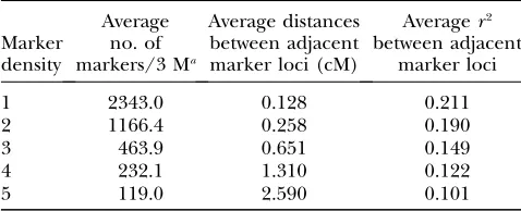
Simulated data: After 10 replicates of each 1000 simulated generations, for the low- and high-heritability trait, on average 78.3 QTL were segregating in gener-ations 1001, 1002, and 1003. The different marker den-sities yielded on average 2343.0, 1166.4, 463.9, 232.1, and 119.0 polymorphic markers across the 3-M genome with distances between adjacent markers averaging from 0.128 to 2.590 cM (Table 1). Average linkage dis-equilibrium between adjacent markers, measured by calculatedr2-values, decreased from 0.211 to 0.101 with increasing average distance between markers (Table 1). The number of haplotypes across the different marker densities was 25–500 times higher for the HAP_IBD models compared to the SNP1 and SNP2 models (Table 2). The number of haplotypes decreased nearly linearly
TABLE 1
Average statistics of the markers of the simulated data sets across the 20 replicates
Marker density
Average no. of markers/3 Ma
Average distances between adjacent marker loci (cM)
Averager2 between adjacent
marker loci
1 2343.0 0.128 0.211
2 1166.4 0.258 0.190
3 463.9 0.651 0.149
4 232.1 1.310 0.122
5 119.0 2.590 0.101
aThe average number of simulated QTL across the 20
with decreasing total number of markers for models SNP1 and SNP2. The number of haplotypes for the HAP_IBD models decreased relatively less with increas-ing total number of markers.
For each of the considered models, a Gibbs chain was run for 600,000 iterations for one of the replicates of the low-heritability trait using the SNP1, SNP2, and HAP_ IBD10 models. The correlation between predicted breeding values for juvenile animals after 30,000 and 600,000 iterations was.0.99. For further analysis 30,000 iterations of the Gibbs sampler were considered to be sufficient, of which 3000 were discarded as burn-in.
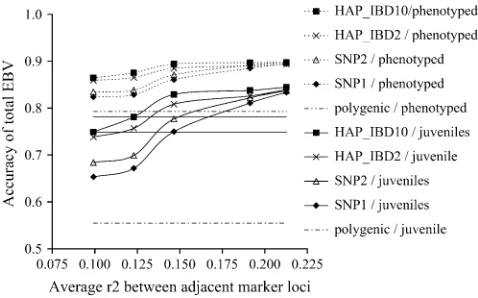
Comparison of simulated and estimated total breeding values: The accuracies of the estimated total breeding values were plotted as a function ofr2-values between adjacent markers (Figures 1 and 2). The accuracies of the estimated breeding values for the high- (low-) her-itability trait using any of the genomic selection models compared to the polygenic model were between 0.03 and 0.10 (0.09 and 0.29) higher for animals with
phenotypes and between 0.10 and 0.29 (0.22 and 0.34) higher for juvenile animals (Figures 1 and 2). Differences in accuracies of estimated breeding values for the high- (low-) heritability trait for phenotyped animals between the different genomic selection mod-els ranged from 0.0 to 0.05 (0.03 to 0.04), whereas for juvenile animals the differences ranged from 0.01 to 0.11 (0.01 to 0.04).
Accuracies of estimated breeding values for the high-heritability trait were across all marker densities, for both phenotyped and juvenile animals, highest for the HAP_IBD10 model and lowest for SNP1 (Figure 1). The differences in accuracies between HAP_IBD and SNP1 were lowest at the highest marker density and were largest at around anr2-value of 0.125 between adjacent markers. When LD between markers decreased, the differences in accuracies between the models increased until an r2-value of 0.12 was reached. For the low-heritability trait, the HAP_IBD10 model yielded the highest accuracies at lower marker densities, but at the highest marker density the accuracy of the SNP1 model was slightly better (Figure 2). Differences between the models were, however, small at all marker densities.
TABLE 2
Number of haplotypes per locus for model HAP_IBD, and average total number of haplotypes for all four models, averaged across the 20 combined replicates of the low- and high-heritability trait
No. of markers
Total no. of haplotypes Average no. of haplotypes per locus
SNP1 SNP2 HAP_IBD2 HAP_IBD10 SNP1 SNP2 HAP_IBD2 HAP_IBD10
2,343.0 4,685 8,022 620,316 192,926 2.0 3.4 264.8 77.0
1,166.4 2,313 4,031 365,231 154,675 2.0 3.5 313.1 123.9
463.9 935 1,652 229,324 128,171 2.0 3.5 494.4 258.8
232.1 474 841 156,443 124,348 2.0 3.6 674.1 491.3
119.0 249 443 129,035 110,574 2.0 3.6 1,085.6 918.7
Figure 1.—Accuracies of total estimated breeding values for the high-heritability trait of phenotyped and juvenile ani-mals estimated with the four different genomic selection models, displayed as a function of differentr2-values for adja-cent marker loci. Standard deviations across replicates ranged from 0.01 to 0.03 for phenotyped animals and from 0.03 to 0.08 for juvenile animals. Coordinates on thex-axis of inter-sections between the model curves and the solid lines indicate the required SNP LD for the different models to obtain accu-racies of 0.75 and 0.78.
The coefficients of the regression of simulated on estimated breeding values were for the high-heritability trait in nearly all cases close to 1.0 for the HAP_IBD model and.1.0 for the SNP1 and SNP2 models (Table 3). This indicates that the SNP models overestimated the total genetic variance when many markers were included,
which is in agreement with the estimated variances (discussed below). The coefficients of the regression of simulated on estimated breeding values were for the low-heritability trait in all cases and for all models,1.0 (Table 3), which is in agreement with the generally overesti-mated total genetic variances (discussed below).
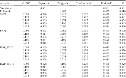
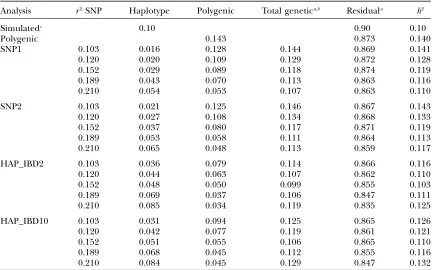
Posterior genetic parameters and QTL probabilities:
Estimated haplotype variances in general increased with increasing marker density for both traits (Tables 4 and 5). For the high-heritability trait, the differences in explained haplotype variance between the models were generally small, and none of the models explained most haplotype variance at all marker densities (Table 4). Estimated haplotype variances for the low-heritability trait were for the HAP_IBD models for all marker den-sities higher than those for the SNP1 and SNP2 models (Table 5). Estimated polygenic variances for both traits tended to be lowest for HAP_IBD2 and highest for SNP1. Estimated residual variances were for both traits and all models close to the simulated value. Standard errors of the estimated variances were for the high-heritability trait at all marker densities smaller for the HAP_IBD models compared to the SNP models, while for the low-heritability trait none of the models had clearly lower standard errors (results not shown).
TABLE 3
Coefficients of regression of simulated on estimated breeding values for animals without phenotypic
records, averaged across 10 replicates with
increasingr2between adjacent markers
Heritability LD SNP SNP1 SNP2 HAP_IBD2 HAP_IBD10
50% 0.099 1.085 1.107 1.009 0.986
0.123 1.127 1.146 1.017 1.003 0.147 1.144 1.140 1.013 0.973 0.191 1.146 1.093 0.993 0.937 0.213 1.137 1.038 0.976 0.896
10% 0.103 0.964 0.971 0.960 0.834
0.120 0.940 0.937 0.950 0.934 0.152 0.922 0.984 0.886 0.894 0.189 0.946 0.974 0.884 0.859 0.210 0.983 0.983 0.920 0.900
SE ranged from 0.009 to 0.053.
TABLE 4
Estimated haplotype, polygenic, total genetic (6SE), and residual (6SE) variances and heritabilities at
different values ofr2between adjacent markers for the high-heritability trait
Analysis r2SNP Haplotype Polygenic Total genetica,b Residuala h2
Simulatedc 0.50 0.50 0.50
Polygenic 0.485 0.455 0.516
SNP1 0.099 0.220 0.412 0.632 0.481 0.543
0.123 0.103 0.379 0.482 0.490 0.491
0.147 0.163 0.274 0.437 0.501 0.454
0.191 0.353 0.150 0.503 0.517 0.463
0.213 0.303 0.090 0.393 0.524 0.420
SNP2 0.099 0.155 0.361 0.516 0.489 0.502
0.123 0.111 0.328 0.439 0.499 0.464
0.147 0.193 0.216 0.409 0.507 0.436
0.191 0.347 0.100 0.447 0.521 0.440
0.213 0.315 0.046 0.361 0.514 0.398
HAP_IBD2 0.099 0.165 0.088 0.253 0.472 0.347
0.123 0.200 0.077 0.276 0.463 0.370
0.147 0.195 0.049 0.244 0.464 0.340
0.191 0.195 0.028 0.222 0.452 0.328
0.213 0.228 0.019 0.247 0.442 0.356
HAP_IBD10 0.099 0.178 0.100 0.278 0.471 0.370
0.123 0.214 0.086 0.299 0.468 0.387
0.147 0.223 0.045 0.268 0.476 0.357
0.191 0.233 0.037 0.269 0.472 0.362
0.213 0.262 0.028 0.290 0.462 0.383
aStandard errors across replicates were calculated as the standard deviation of the estimated variances
di-vided bypffiffiffiffiffi10and ranged from 0.013 to 0.102 for the total genetic variance and from 0.009 to 0.020 for the residual variance.
bThe sum of estimated QTL and polygenic variances.
Estimated heritabilities for the high-heritability trait were especially underestimated by the HAP_IBD models. The heritability estimates of the SNP1 and SNP2 models were closer to the simulated variance, but decreased with increasing marker density. For the low-heritability trait, all models slightly overestimated the heritability.
In Figure 3, the ratio of cumulated estimated haplo-type variance to total simulated QTL variance, across loci with decreasing estimated haplotype variance, is plotted against the cumulative number of loci for marker densities withr2between markers of 0.15 (Figure 3, A and C) and 0.21 (Figure 3, B and D). The points of the curves at the largest number of loci indicate the pro-portion of the simulated QTL variance that is explained by the total estimated haplotype variance across all loci;
i.e., at marker densities withr2between markers of 0.15 and 0.21, respectively, the estimated haplotype variances explained across models on average 38 (Figure 3A) and 54% (Figure 3B) of the simulated QTL variance for the trait with high heritability and 41 (Figure 3C) and 71% (Figure 3D) of the simulated QTL variance for the trait with low heritability. The initial steep progression of the curves indicates that at low marker density in all models a large proportion of the total estimated haplotype variance is fitted on a limited number of loci (Figure 3, A
and C). At high marker density, still a few loci have a large estimated variance, but the contribution of these loci to the total explained haplotype variance is less (Figure 3, B and D). The linear progression of the curves for the HAP_IBD models in Figure 3, following the steep initial progression, indicates that for all situations most of the loci in the HAP_IBD models explain more or less the same amount of variance. The curvilinear progression of the curves for the SNP models, following the steep initial progression, indi-cates that the contribution of loci to the total estimated haplotype variance for the SNP models eventually be-comes smaller. The average posterior probabilities that a QTL was sampled at a locus, for 30 loci with the highest posterior probabilities, are plotted in Figure 4. These results show that for the high-heritability trait the HAP_IBD models sampled QTL with a high posterior probability at a few loci, while the SNP models had much lower posterior probabilities on the loci with the largest estimated haplotype variance (Figure 4A). For the low-heritability trait, average posterior probabilities were much lower for the loci that had the largest estimated haplotype variance, and the highest average posterior probability was actually found for the SNP1 model (Figure 4B).
TABLE 5
Estimated haplotype, polygenic, total genetic (6SE), and residual (6SE) variances and heritabilities at
different values ofr2between adjacent markers for the low-heritability trait
Analysis r2SNP Haplotype Polygenic Total genetica,b Residuala h2
Simulatedc 0.10 0.90 0.10
Polygenic 0.143 0.873 0.140
SNP1 0.103 0.016 0.128 0.144 0.869 0.141
0.120 0.020 0.109 0.129 0.872 0.128
0.152 0.029 0.089 0.118 0.874 0.119
0.189 0.043 0.070 0.113 0.863 0.116
0.210 0.054 0.053 0.107 0.863 0.110
SNP2 0.103 0.021 0.125 0.146 0.867 0.143
0.120 0.027 0.108 0.134 0.868 0.133
0.152 0.037 0.080 0.117 0.871 0.119
0.189 0.053 0.058 0.111 0.864 0.113
0.210 0.065 0.048 0.113 0.859 0.117
HAP_IBD2 0.103 0.036 0.079 0.114 0.866 0.116
0.120 0.044 0.063 0.107 0.862 0.110
0.152 0.048 0.050 0.099 0.855 0.103
0.189 0.069 0.037 0.106 0.847 0.111
0.210 0.085 0.034 0.119 0.835 0.125
HAP_IBD10 0.103 0.031 0.094 0.125 0.865 0.126
0.120 0.042 0.077 0.119 0.861 0.121
0.152 0.051 0.055 0.106 0.865 0.110
0.189 0.068 0.045 0.112 0.855 0.116
0.210 0.084 0.045 0.129 0.847 0.132
aStandard errors across replicates were calculated as the standard deviation of the estimated variances
di-vided bypffiffiffiffiffi10and ranged from 0.003 to 0.010 for the total genetic variance and from 0.002 to 0.008 for the residual variance.
bThe sum of estimated QTL and polygenic variances.
DISCUSSION
The aim of this study was to compare the accuracy of predicted breeding values using four different models to estimate total breeding values for genomic selection. The results confirmed that genomic selection, com-pared to traditional selection based solely on pedigree information, is especially for a trait with low heritability considerably more accurate for juvenile animals, even at an average r2-value between adjacent markers of 0.10 and when using relatively simple models. The benefit is such that accuracies of total genomic breeding values for juvenile animals were actually in most cases higher than those of traditional breeding values for animals with known phenotypic information. Although esti-mated haplotype variance at a few loci explained a rela-tively large part of the simulated QTL variance, a large part of the total estimated haplotype variance was ex-plained by loci that had an average posterior QTL prob-ability,0.01. This suggests that parts of the genome, for which no clear evidence exists for the presence of a QTL, still explain an important part of the genetic variance in applications of genomic selection.
Meuwissen et al. (2001) discussed that their
simu-lated microsatellite markers, spaced at 1-cM distances, resembled approximately three to five SNP markers. Thus, their marker distance of 1 cM would be compa-rable to the average distance between SNP markers of 0.26 cM in our study. The correlation between simulated and estimated breeding values of 0.82 for the high-heritability trait using model SNP2 in our study was comparable to the correlation of 0.79 reported by Meuwissen et al. (2001) when their breeding values
were estimated on the basis of 1000 animals with phe-notypes for a trait with heritability of 50%. Solberget al.
(2006) applied genomic selection to simulated data, estimating effects of single-marker alleles comparable to our SNP1 model for a trait with heritability of 50%. At marker distances of 1 and 0.5 cM the accuracies of their estimated breeding values were respectively 0.66 and 0.72, comparable to accuracies in our study of 0.67 and 0.75 at marker distances of respectively 1.3 and 0.65 cM. It should be noted that in our study polygenic effects were included in the model, whereas they were not in the studies by Meuwissen et al. (2001) and Solberg
et al. (2006). Reported r2-values between markers of $0.3 in, for instance, dairy and beef cattle (Hayeset al.
2006) are comparable to ther2-values in our simulations and indicate a large potential benefit of applying ge-nomic selection. It should, however, be noted that our simulated markers were relatively uniformly distributed, while commercially available SNPs might be less
formly distributed. This implies that next to the LD between adjacent markers, also the distribution of the markers along the genome has to be taken into account to predict the potential benefit of genomic selection.
Four different models were compared in this study. The HAP_IBD2 and SNP2 models both used two markers to construct haplotypes, with the difference that the HAP_IBD2 model included IBD probabilities between different haplotypes. Thus, in the HAP_IBD2 model different linkage phases between marker hap-lotypes and QTL are considered in different (families of) animals, while the SNP2 approach assumes that a certain marker haplotype is always linked to the same QTL allele. The differences found in this study indicate that including linkage analysis information in the model considerably increases the accuracy of breeding values for a high-heritability trait. For the low-heritability trait, there was little difference between the models across the range of marker densities.
Adding additional markers in the HAP_IBD model slightly improved the accuracy for both traits at all marker densities. For QTL mapping, it has been shown that predictive ability of an IBD-based model was largest
for an intermediate number of markers; i.e., at some stage additional markers led to lower predictive ability of the model (Grapes et al. 2006). Since in our study
only two haplotype sizes were considered, it remains unclear whether for genomic selection applications the accuracy of IBD models also is highest at an optimal number of markers or is not.
None of the models was clearly superior for the low-heritability trait. The most striking observation is that the SNP1 model yielded the lowest accuracy at low marker density and the highest accuracy at high marker density. To investigate this apparent inconsistency, we compared the results between the different models at different marker densities within replicates. Results of all replicates for the SNP1 and HAP_IBD10 models, as well as the average accuracy, are shown in Figure 5 for marker densities with r2between adjacent markers of 0.15 and 0.21. Results in, for instance, replicates 4 and 6 appeared to be rather inconsistent, as the SNP1 model was clearly superior at the highest marker density, while at the other marker density (r2¼0.15) the SNP1 model was clearly inferior (see dashed lines in Figure 5). In replicate 4, the SNP1 model found at the highest marker density the highest posterior probability for a QTL that explained 35% of the simulated genetic vari-ance, while at the lower marker density the other models found higher posterior probabilities for this QTL. In replicate 6, at the lower SNP density a few important SNP were lost that disabled the SNP1 model to detect a very large QTL that explained 75% of the simulated genetic variance. The other three models, however, were still well able to pick up this QTL. Having a QTL that explained such a large amount of variance,i.e., both the simulated QTL effect and the heterozygosity (0.47) were large, replicate 6 was rather extreme. However, when discarding the results from replicate 6, the SNP1
Figure4.—Average posterior probabilities for the 30 loci with the largest (decreasing) estimated haplotype variance for the trait withh2¼ 50% (A) andh2 ¼10% (B), both at the highest SNP density.
and HAP_IBD10 models on average gave similar results. Thus, at higher marker density, the SNP1 model may actually yield the highest accuracy when some SNPs are (expected to be) closely linked to some important QTL, while the HAP_IBD models are a better choice if there are no SNPs (expected to be) closely linked to impor-tant QTL.
The main disadvantage of the HAP_IBD models is that the number of effects that needs to be estimated is considerably larger than that for the SNP models. Still, the HAP_IBD2 model was able to accurately estimate total breeding values, using only 1100 phenotypic re-cords, but based on up to 2100 polygenic and 620,316 haplotype effects. The number of haplotype effects that needs to be estimated can be reduced by including more markers per haplotype and perhaps by clustering of haplotypes that have an IBD probability of, for in-stance,.0.80. Reduction of the number of haplotypes not only improves the feasibility, but also may improve the power of the model.
In Figure 1, the top horizontal solid line indicates that the accuracy for juvenile animals of the HAP_IBD10 model for the high-heritability trait at r2 between ad-jacent markers of 0.12 was comparable to the accuracy obtained with the SNP2 model at anr2between adjacent markers of 0.15. The bottom horizontal solid line in-dicates that the accuracy for juvenile animals of the HAP_IBD10 model at an r2 between markers of 0.10 was comparable to the accuracy obtained with the SNP2 model at anr2between markers of 0.14. Translated into numbers of markers in our simulated data sets, in the most extreme situations the SNP2 model needed two to three times as many markers to yield the same results as the HAP_IBD10 model for the high-heritability trait.
In conclusion, there is a clear advantage of genomic selection even at low marker densities and using a sim-ple model that uses marker alleles as haplotypes. Unless there is an expectation that some SNPs are in high linkage disequilibrium with large QTL, the HAP_IBD model is the safest option. However, the results suggest that probably a combination of using alleles of SNPs that have a known effect in combination with reconstructed
haplotypes for the parts of the genome with unknown effect might prove to be the best solution.
The authors thank John Bastiaansen, Egbert Knol, Chris Schrooten, and Addie Vereijken for their suggestions and comments on the results of this study. Hendrix Genetics, HG B.V. (formerly known as Holland Genetics), Institute for Pig Genetics, and SenterNovem are acknowledged for financial support.
LITERATURE CITED
Falconer, D. S., and T. F. C. Mackay, 1996 Introduction to
Quantita-tive Genetics.Longman Group, Essex, UK.
Fernando, R. L., and M. Grossman, 1989 Marker assisted selection
using best linear unbiased prediction. Genet. Sel. Evol.21:467–477. Grapes, L., J. C. M. Dekkers, M. F. Rothschildand R. L. Fernando,
2004 Comparing linkage disequilibrium-based methods for fine mapping quantitative trait loci. Genetics166:1561–1570. Grapes, L., M. Z. Firat, J. C. M. Dekkers, M. F. Rothschildand R. L.
Fernando, 2006 Optimal haplotype structure for linkage
dis-equilibrium-based fine mapping of quantitative trait loci using identity by descent. Genetics172:1955–1965.
Hayes, B. J., A. J. Chamberlainand M. E. Goddard, 2006 Use of
markers in linkage disequilibrium with QTL in breeding pro-grams. Proceedings of the 8th World Congress on Genetics Applied to Livestock Production, Belo Horizonte, MG, Brazil, Communication 30–06.
Meuwissen, T. H. E., and M. E. Goddard, 2000 Fine mapping of
quantitative trait loci using linkage disequilibria with closely linked marker loci. Genetics155:421–430.
Meuwissen, T. H. E., and M. E. Goddard, 2001 Prediction of
iden-tity by descent probabilities from marker-haplotypes. Genet. Sel. Evol.33:605–634.
Meuwissen, T. H. E., and M. E. Goddard, 2004 Mapping multiple
QTL using linkage disequilibrium and linkage analysis informa-tion and multitrait data. Genet. Sel. Evol.36:261–279. Meuwissen, T. H. E., B. J. Hayesand M. E. Goddard, 2001
Pre-diction of total genetic value using genomewide dense marker maps. Genetics157:1819–1829.
Schaeffer, L. R., 2006 Strategy for applying genome-wide selection
in dairy cattle. J. Anim. Breed. Genet.123:218–223.
Solberg, T. R., A. K. Sonesson, J. A. Woolliams and T. H. E.
Meuwissen, 2006 Genomic selection using different marker
types and density. Proceedings of the 8th World Congress on Genetics Applied to Livestock Production, Belo Horizonte, MG, Brazil, Communication 22–13.
Windig, J. J., and T. H. E. Meuwissen, 2004 Rapid haplotype
recon-struction in pedigrees with dense marker maps. J. Anim. Breed. Genet.121:26–39.
Xu, S. Z., 2003 Estimating polygenic effects using markers of the
en-tire genome. Genetics163:789–801.