DEPARTMENT OF STATISTICS North Carolina State University
2501 Founders Drive, Campus Box 8203 Raleigh, NC 27695-8203
Institute of Statistics Mimeo Series No. 2573
August 2004
Multiclass Proximal Support Vector Machines
Yongqiang Tang Hao Helen Zhang
Department of Statistics, North Carolina State University, Raleigh, NC
ytang,[email protected]
MULTICLASS PROXIMAL SUPPORT VECTOR MACHINES
YONGQIANG TANG, HAO HELEN ZHANG
Abstract. We propose an extension of proximal support vector machines (PSVM) to the
multi-class case. Unlike the one-versus-rest approach that constructs the decision rule based on multiple
binary classification tasks, the multiclass PSVM (MPSVM) considers all classes simultaneously and
provides a unifying framework when there are either equal or unequal misclassification costs. The
MPSVM is built in a regularization framework of reproducing kernel Hilbert space (RKHS) and
implements the Bayes rule asymptotically. With regard to computation, the MPSVM simply solves
a system of linear equations and demands much less computational effort than the SVM, which can
be slow due to optimizing a large-scaled quadratic programming under linear constraints. Some
effi-cient algorithm is suggested and one stable computation strategy is also provided for ill-posed cases.
The effectiveness of the MPSVM was demonstrated by both simulation studies and applications to
cancer classification using microarray data.
1. Introduction
Consider the multiclass classification problem with class labels {1, . . . , k}. Given a training set {(xi, yi), i= 1, . . . , n}, wherexi ∈ <d is the measurement vector and yi is the class label, our task is to learn a classification rule from the training set to predict the true class of a future object by only observing its measurement vector. Support vector machine (SVM) (Boser et al. (1992), Vapnik (1998), Burges (1998), and Cristianini and Shawe-Taylor (2000)) has shown successful performances in various studies. What makes the SVM attractive is its ability to condense the information contained in the training set and to find a decision surface determined by certain
Key words and phrases. Bayes optimal classification rules, Nonstandard classifications, Reproducing kernel Hilbert space.
Dr. Hao Helen Zhang’s research is partially supported by NSF Grant DMS-0405913.
points of the training set. Lee et al. (2004) further generalized the SVM to multicategory SVM (MSVM).
The implementation of the SVM or MSVM demands solving a quadratic programming under linear constraints. For large datasets, solving a constrained quadratic problem is generally compu-tational expensive. In the case of a multiclass classification, the computation can be challenging even for a moderate-size dataset with many classes. Proximal support vector machines (PSVM) was introduced recently as a variant of SVM for binary classifications in Suykens and Vandewalle (1999) and Fung and Mangasarian (2001b). In theory, both PSVM and SVM asymptotically target on the optimal Bayes rule, which explains their comparable prediction accuracies in most empirical studies. More importantly, the PSVM solves a system of linear equations using an extremely fast and simple algorithm and thus demands much less computational effort than the SVM. The least squares SVM (Suykens and Vandewalle (1999), Suykens et al. (2002) and Van Gestel et al. (2002a)) has similar loss functions as the PSVM except that the latter penalizes the constant term as well. Several proposals for multiclass PSVM and least squares SVM are based on the one-versus-rest scheme, which essentially transforms the multiclass separation into k binary classifications by ar-tificially relabeling the data and constructing decision rules according to the maximal output. See Van Gestel et al. (2002b) and Fung and Mangasarian (2001a) for details.
The multiclass PSVM (MPSVM) proposed in this paper targets directly on the boundary among k classes by estimating some functions ofk conditional probabilities simultaneously. The MPSVM is constructed in a regularization framework of reproducing kernel Hilbert space (RKHS) and it is optimal in terms of implementing Bayes rule asymptotically. Compared to the approaches based on the one-versus-rest scheme, the MPSVM is more flexible to handle nonstandard situations where there are unequal misclassification costs or nonpresentative training sets. With regard to computation, the MPSVM can be solved more efficiently than the MSVM.
The paper is organized as follows. We briefly review the Bayes classification rule in Section 2 and the binary SVM and PSVM in Section 3. In Section 4, we introduce the MPSVM, study its statistical properties and present two computation algorithms. Section 5 illustrates the performance of MPSVM with simulation examples. In Section 6, the MPSVM is applied to cancer classifications using gene expression data.
2. Bayes classification rules
The Bayes rule is the optimal classification rule if the underlying distribution of the data is known. They serve as golden standards for any reasonable classifiers to approximate. In practice, the underlying distribution is rarely known. One common way to approximate the Bayes rules is to estimate the distribution or related classification functions from the training set.
For ak-class classification problem, we need to learn a classification ruleφ(x) :<d → {1, . . . , k}. Assume that observations in the training data are i.i.d. and drawn from some distributionP(x, y). Letpj(x) = Pr(Y =j|X=x) be the conditional probability of classjgivenX=xforj = 1, . . . , k. Let C be ak×k cost matrix with entry Cjl meaning the cost paid for classifying an observation from class j to class l. All Cjj (j= 1, . . . , k) should equal 0 since the correct decision should not be penalized. The Bayes rule, minimizing the expected cost of misclassifying an observation
E
CY φ(X)
=EX
" k X
l=1
Clφ(x)Pr(Y =l|X=x)
#
=EX
" k X
l=1
Clφ(x)pl(x)
#
,
is given by
(1) φB(x) = arg min
j=1,...,k
" k X
l=1
Cljpl(x)
#
.
When the misclassification costs are all equal, that is, Clj = 1 if j6=l, the Bayes rule simplifies to
(2) φB(x) = arg min
j=1,...,k[1−pj(x)] = arg maxj=1,...,kpj(x),
The majority of classification methods is “standard” in the sense that the samples in the training set represent some target population and the costs of different misclassifications are the same. However, nonstandard classifications may arise in many real situations. See Lin et al. (2002). One typical situation is that some type of misclassifications may be more serious than others and unequal misclassification costs should be assumed. For example, in the diagnosis of disease, considering a healthy person classified as sick or a sick patient as healthy may have different consequences. Sampling bias is another issue that needs special attention (Lin et al. (2002) and Lee et al. (2004)). In many studies where the proportions of each class in the true population were extremely unbalance, the minor classes were usually over-sampled and major classes were usually down-sampled. If the sampling scheme depends only on the class labels Y, and not on the measurements X, the Bayes rule is
φB(x) = arg min j=1,...,k
" k X
l=1 πl πs l
Cljpsl(x)
#
,
whereπl is the proportion of class l in the target population,πls is the proportion of class l in the training set, andpsl(x) = Pr (Ys=l|Xs=x) is the conditional probability that a sample randomly drawn from the training set belongs to class l given Xs = x (Lee et al. (2004)). A remedy for sampling bias is to define the new misclassification costs according to
(3) Cjlnew=Cjl
πl πs l
.
In this paper, we call a classification problem “nonstandard” if misclassification costs are not all equal or there is a sampling bias. We are not going to differentiate the two nonstandard cases since the issue of sampling bias could be handled by defining new costs according to (3).
3. Binary SVM and PSVM
In binary classification problems, the class labels yi are often coded as {+1,−1}. The SVM is motivated by the geometric interpretation of maximizing the margin. It has been shown that SVM
methodology can be cast as a regularization problem in a reproducing kernel Hilbert space (RKHS). See Wahba (1990), Girosi (1998), and Poggio and Girosi (1998). Lin et al. (2002) extended SVM to the nonstandard case. Let HK be an RKHS with reproducing kernel K. The SVM for both standard and nonstandard classifications solves
(4) min
f 1 n
n
X
i=1
L(yi)(1−yif(xi))++λkhk2HK,
over all the functions of the form f(x) =h(x) +β0, where h ∈ HK, (v)+ = max{v,0}, and L(yi) is the cost for misclassifying the i-th observation. The classification rule is sign[f(x)].
Suykens and Vandewalle (1999) and Fung and Mangasarian (2001b) proposed PSVM, which classifies the points by assigning them to the closest of two parallel planes in input or feature space that are pushed apart as far as possible. In an RKHS, the PSVM could be formulated as
(5) min
f 1 n
n
X
i=1
L(yi)[1−yif(xi)]2+λ(khk2HK +β
2 0).
Since eachyi= 1 or −1, formulation (5) is equivalent to
(6) min
f 1 n
n
X
i=1
L(yi)[yi−f(xi)]2+λ(khk2HK +β02).
Thus PSVM could be interpreted as the Ridge regression model (Agarwal (2002)).
By the representer theorem ( Kimeldorf and Wahba (1971) and Wahba (1999)), the solutions to (4) and (5) have a representation of the form
f(x) =β0+ n
X
i=1
βiK(xi,x),
where{βi}n
i=0∈ <. The RKHS framework is closely related to the well-known kernel methodology. The fact that for any positive definite kernel, there exists a unique RKHS is well established by the Moore Aronszjantheorem (Aronszajn (1950)).
When K(xi,xl) =<xi,xl >orh(x) = ˜βx and misclassification costs are all equal, formulation (5) is equivalent to
min f
1 n
n
X
i=1
[1−yi(β0+ ˜βx)]2+λ(kβ˜k2+β02).
This is the linear PSVM studied in Suykens and Vandewalle (1999) and Fung and Mangasarian (2001b). In general, the formulation (5) under equal misclassification costs reduces to
(7) min
f 1 n
n
X
i=1
[1−yif(xi)]2+λ
n
X
j=1 n
X
l=1
βjβlK(xj,xl) +β02
.
Formulation (7) is slightly different from the original kernel PSVM (equation (19), Fung and Man-gasarian (2001b)), which is equivalent to
min f
1 n
n
X
i=1
[1−yif(xi)]2+λ
n
X
j=1
βj2+β02
.
One strategy for constructing multiclass classifiers is to transform the multiclass classification problem into a series of binary subproblems. For SVM-type classifiers, one-vs-rest scheme has been widely used to handle the multiclass classification problems (Van Gestel et al. (2002b) and Fung and Mangasarian (2001a)). The general idea of this scheme is to solve k binary subproblems, each trained to separate one class from the rest, and to construct decision rules according to the maximal output. One disadvantage of one-versus-rest scheme is that the resulting two-class subproblems are often very unbalanced, leading to poor performances in some cases (Fung and Mangasarian (2001a)). In addition, it is not easy to take into account unequal misclassification costs in the one-versus-rest scheme. One alternative strategy is to separate all thekclasses simultaneously instead of classifying one from the rest. In fact, it has been used to formulate multiclass SVM classifiers such as in Vapnik (1998), Weston and Watkins (1999), and Lee et al. (2004). These methods generally need to solve a quadratic programming with linear constraints. For large datasets, the computation effort can be very expensive.
4. Multiclass PSVM
We propose an extension of PSVM to the multiclass case. The MPSVM embraces the binary PSVM as a special case. In Section 4.1, we present the formulation of MPSVM, investigate the properties of its solution and study its asymptotic classification performance. Section 4.2 introduces two efficient computational strategies for implementing the MSPVM.
4.1. The formulation and theoretical properties. In the multiclass problem, the class label is coded as a k-dimensional vector
yi =
1,k−−11, . . . ,k−−110if observation iis in category 1,
−1
k−1,1, . . . ,k−−11
0
if observation iis in category 2,
. . .
−1
k−1,k−−11, . . . ,1
0
if observation iis in category k.
We define ak-tuple of separating functionf(x) = (f1(x), . . . , fk(x))0. Since the sum of components in eachyis 0, we letf satisfy the sum-to-zero constraint,Pk
j=1fj(x) = 0 for anyx∈ <d. Analogous to the binary case, we considerf(x)∈Qk
j=1({1}+HK), the product space ofk reproducing kernel Hilbert spaces HK. In other words, each component fj(x) can be expressed as hj(x) +βj0, where hj ∈ HK and βj0 ∈ <. Define the diagonal matrix W(yi) = diag{Cj1, Cj2, . . . , Cjk} where Cjl (l = 1, . . . , k) are the costs of classifying thei-th observation from class j to class l ifyi indicates classj. The MPSVM is proposed as minimizing
(8) 1
n n
X
i=1
(yi−f(xi))0W(yi)(yi−f(xi)) + 1 2λ
k
X
j=1
(||hj||2HK +b
2 j),
subject toPk
j=1fj(x) = 0 for anyx. The classification rule induced byf(x) isφ(x) = arg maxjfj(x). This formulation handles the standard and nonstandard classifications in a unified way.
The functional form of the solutions to (8) is given by the following representer theorem. Proof of this theorem and all other proofs are given in the appendix.
Theorem 1. Representer TheoremIf the reproducing kernel K is positive definite, minimizing
(8) under the sum-to-zero constraint is equivalent to finding f1(x), . . . , fk(x)
of the form
(9) fj(x) =βj0+
n
X
i=1
βjiK(xi,x),
subject to Pk
j=1βjl= 0 for l= 0, . . . , n.
The formulation (8) embraces the binary PSVM as a special case. To verify this, we will show that the data fit functionals and penalties of model (6) and (8) are identical when k = 2. When yi = (1,−1) (1 in the binary notation), then W(yi) = diag{0, L(1)} and (yi−f(xi))0W(yi)(yi− f(xi)) =L(1)(f2(xi) + 1)2 =L(1)(1−f1(xi))2, where L(1) is the cost of misclassifying a positive sample. Similarly, whenyi= (−1,1) (−1 in the binary notation), we haveW(yi) = diag{L(−1),0} and (yi−f(xi))0W(yi)(yi−f(xi)) =L(−1)(−1−f1(xi))2, whereL(−1) is the cost of misclassifying a negative sample. Thereby, the data fit functionals in (6) and (8) are identical, f1(x) playing the same role asf(x) in (6). Also, note that λ2P2
j=1(||hj||2HK+β
2
j0) = λ2(||h1||2HK+β
2
10+||h2||2HK+β
2 20) = λ(||h1||2HK+β102 ) sinceβ10+β20= 0 andh1(x)+h2(x) = 0 for anyxby Theorem 1. So the penalties to the model (6) and (8) are also identical.
Theorem 2 says that the proposed MPSVM implements Bayes rule asymptotically under certain regularity conditions. We use the theoretical framework Cox and O’Sullivan (1990) for analyz-ing the asymptotics of penalized methods, which had been used to study the SVM and MSVM (Lin (2002) and Lee et al. (2004)). In the formulation (8), the data fit functional component in-dicates that the estimate should follow the pattern in the data, whereas the penalty component imposes smoothing conditions. The limit of the data fit functional as the sample size goes to in-finity, E[(Y −f(X))0W(Y)(Y −f(X))], could be used to identify the target function, which is
the minimizer of the limiting functional. Under the assumption that the target function can be approximated by the elements in the RKHS and certain other regularity conditions, the solution to (8) will approach the target function as n→ ∞.
Theorem 2. The minimizer ofE[(Y −f(X))0W(Y)(Y −f(X))]under the sum-to-zero constraint is implements the Bayes rule, that is
arg max
j=1,...,kfj(x) =argj=1min,...,k k
X
l=1
cljpl(x).
In particular, under equal misclassification costs, argmaxj=1,...,kfj(x) =argmaxj=1,...,kpj(x).
Remark 3. Inversing (23) in the appendix yields an estimate of the class probabilities. When misclassification costs are all equal, τj(x) reduces to 1−pj(x) and
(10) pˆj(x) = 1−(k−1)
1/(1−fjˆ(x))
Pk
l=11/(1−fˆl(x)) ,
for each j= 1, . . . , k.
4.2. Computation Algorithms. Compared to SVM and MSVM, the MPSVM simply solves a system of linear equations and demands much less computational effort. Most classification methods involve parameters that are often predetermined by some tuning strategies such as cross-validation. The computational advantage of the MPSVM makes it possible to perform a finer search of these parameters, which may lead to better results. The speed of the MPSVM makes it also very promising for analysis of large data sets. In this section, two computation strategies are presented and summarized in Algorithm 1 and 2. We assume the kernel K is strictly positive definite. Algorithm 1 runs fast, however it may fail when K is close to singularity since it is impossible or difficult to inverse K numerically. Algorithm 2 is specifically designed to prevent the ill-posed situations.
Let ˆKbe then×nmatrix withilentryK(xi,xl). LetZ = [1n K] andˆ G=
1 00n 0n Kˆ
, where
1n = (1, . . . ,1)0 and 0n = (0, . . . ,0)0. For each j = 1, . . . , k, define vectors y∗j = (y1j, . . . , ynj)0,
cat{l} is the class the l-th observation belongs to, and Ccat{l}j is the cost of classifying the l-th observation as class j. Let λ∗ = nλ/2, β∗j = G1/2βj, Z∗ = ZG−1/2, Zj = Wj∗1/2Z∗ and y∗∗j =Wj∗1/2y∗j forj = 1, . . . , k. By Theorem 1, minimizing (8) is equivalent to minimizing
k
X
j=1
(y∗j −Zβj)0Wj∗(yj∗−Zβj) +λ∗β0jGβj
(11) = k X j=1
(y∗∗j −Zjβ∗j)0(y∗∗j −Zjβ∗j) +λ∗β∗j0β∗j
(12)
subject to Pk
j=1βj =
Pk
j=1β∗j =0n+1.
To solve (12), we consider its Wolfe dual problem
LD = k
X
j=1
(y∗∗j −Zjβ∗j)0(y∗∗j −Zjβ∗j) +λ∗β∗j0β∗j
−2u∗0 k
X
j=1 β∗j,
whereu= 2u∗∈ <n+1 is the Lagrange multiplier.
Setting equal to zero the gradient of LD with respect to β∗j yields
∂LD ∂β∗j = 2Zj
0(Z
jβ∗j −y∗∗j ) + 2λ∗β∗j −2u∗= 0.
Thus
(13) β∗j = Zj0Zj+λ∗I
−1
Zj0y∗∗j +u∗=Bj Zj0y∗∗j +u∗
,
whereBj =Zj0Zj+λ∗I−1 forj= 1, . . . , k. Since 0n+1=Pkj=1β∗j =
Pk
j=1Bj
Z0
jy∗∗j +u∗
, we get
(14) u∗=−
k X j=1 Bi
−1
k
X
j=1
BjZj0y∗∗j
.
The solution to (11) is given by
(15) βj =G−1/2β∗j =Aj Z0Wj∗y∗j+v
,
whereAj =G−1/2BjG−1/2 =
Z0W∗
jZ+λ∗G
−1
and v=−Pk
j=1Ai
−1 Pk
j=1AjZ0Wj∗y∗j
For any (new) observation x, define the vector Kx = [K(x,x1), . . . , K(x,xn)]0. Algorithm 1 could be summarized as follows.
ALGORITHM 1. (1) Solve (11) using (15).
(2) To predict a (new) sample, compute fjˆ(x) = [1, Kx0]βj for j= 1, . . . , k and classify the sample to the class giving the largest fˆj(x).
In theory, the matrix ˆKis strictly positive definite. However, in practice it can be numerically ill-posed. Algorithm 1 may fail when ˆK, and henceGand Aj (j= 1, . . . , k), are close to singularities. In Algorithm 2, the inversion of G is avoided by using ZG−1 = [1
n, I] and ZG−1Z0 = 1n10n+ ˆ
K, which is achieved by some strategic matrix transformation of the solution given in (13) and
(14) via the Sherman-Morrison-Woodbury formula. Our experience shows that, when ˆK is good-conditioned, we should use Algorithm 1 since it is much more efficient than Algorithm 2; otherwise Algorithm 2 provides an alternative way to get the solution.
By the use of Sherman-Morrison-Woodbury formula,
(16) Bj = Zj0Zj+λ∗I
−1
= 1/λ∗
I−Zj0(λ∗I+ZjZj0)−1Zj
= 1/λ∗(I−Z∗0CjZ∗),
where
(17) Cj =Wj∗1/2
h
λ∗I+Wj∗1/2Z∗Z∗0Wj∗1/2i−1Wj∗1/2 =lj
λ∗I+lj Z∗Z∗0−1
,
lj be the column vector containing the diagonal elements of Wj∗1/2, lj =ljl
0
j, and is the elemen-twise products of two matrices.
It is easy to verify that
(18) BjZj0y∗∗j = 1/λ∗
I−Zj0(λ∗I+ZjZj0)−1Zj
LetC = 1/kPk
j=1Cj. Then
(19) B =
k
X
j=1
Bj =k/λ∗(I−Z∗0CZ∗).
By the Sherman-Morrison-Woodbury formula,
(20) B−1 =λ∗/k
I−Z∗0(Z∗Z∗0−C−1)−1Z∗
.
Combining equations (14), (20) and (18), we get
u∗ =−B−1
k
X
j=1
BjZj0y∗∗j
=−λ∗/k(I−Z∗0DZ∗)
Z∗0
k
X
j=1 Cjy∗j
=−λ∗Z∗0Q, (21)
whereD = (Z∗Z∗0−C−1)−1, H= 1/kPk
j=1Cjy∗j, and Q=H−D(Z∗Z∗0)H =−DC−1H. By equations (14), (21), (18) and (16),
β∗j =BjZj0y∗∗j +Bju∗=Z∗0Cjy∗j−(I−Z∗0CjZ∗)Z∗0Q=Z∗0
Cj(y∗j+Z∗Z∗0Q)−Q
.
Hence
βj =G−1/2βj∗=G−1/2Z∗0
Cj(y∗j +Z∗Z∗0Q)−Q
= [1n, I]0
Cj(y∗j+Z∗Z∗0Q)−Q
.
The prediction of ˆfj forxis given by
(22) fˆj(x) = [1, Kx0]βj = (1n+Kx)
Cj(y∗j +Z∗Z∗0Q)−Q
.
ALGORITHM 2. (1) ComputeZ∗Z∗0=ZG−1Z0 =1n10n+ ˆK
(2) Compute Cj (j= 1, . . . , k),C, D, H andQ as defined in (17) and (21).
(3) To predict a (new) sample, compute fˆj(x) for j = 1, . . . , k using (22) and classify the sample to the class giving the largest fˆj(x).
5. Numerical examples
We illustrate the MPSVM by simulation studies in this section and analysis of microarray data in the next section. Throughout, the Gaussian kernel K(xi,xl) = exp
−kxi−xlk2 σ2
was used and (λ∗, σ2) was determined by the use of 10-fold cross-validation. Section 5.2 illustrated an example on nonstandard classifications. In all other examples, equal misclassification costs were assumed.
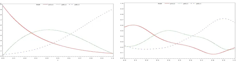
5.1. Comparison with MSVM using simulation. Similar to Lee et al. (2004), a training set of sample size 200 was simulated according to the three-class model on the unit interval [0,1] with the conditional probabilities p1(x) = 0.97 exp(−3x), p3(x) = exp −2.5(x−1.2)2, and p2(x) = 1−p1(x) −p3(x). We applied the MPSVM to the simulated data and used (10) to estimate the conditional probabilities. Figure 1(a) and 1(b) depicted the true and estimated conditional probabilities, respectively. The MPSVM recovered the shape of the true probability functions to some extent. According to (2), the Bayes class boundaries were atx= 0.260 wherep1(x) =p2(x)> p3(x) and x = 0.613 where p1(x) < p2(x) = p3(x) while the two critical points estimated by the MSPVM were around 0.262 and 0.615. So the MPSVM classifier approximate the Bayes optimal rule reasonably well.
(a) The true conditional probabilities (b) The probabilities estimated by MPSVM
Figure 1. The true and estimated conditional probability functions
To compare with the MSVM, we simulated 100 replicate training datasets of sample size 200 and a testing dataset of sample size 10000 and applied MPSVM and one-versus-rest PSVM to each training set. The trained classification rules were then used to evaluate the testing error rates over the testing data. The Bayes optimal classification error rates was 0.3841, whereas the average testing error rate (± standard deviation) over 100 replicates was 0.4068±0.0101 by the MPSVM, and 0.4081±0.0124 by the one-versus-rest PSVM. The same simulation strategy was used to evaluate the MSVM and one-versus-rest SVM in Lee et al. (2004), where the average testing error rate was 0.3951±0.0099 by the MSVM, and 0.4307 ±0.0132 by the one-versus-rest SVM. The performances of PMSVM and one-versus-rest PSVM were almost as good as that of MSVM. The error rate by the one-versus-rest SVM was a little higher. One possible reason was that the one-versus-rest SVM may not approximate the Bayes rule well even when the sample size gets large (Lee et al. (2004)), while all other three classifiers are asymptotically optimal.
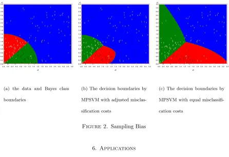
5.2. Sampling bias. To illustrate the effective of MPSVM in handling sampling bias, we firstly simulated a sample of size 500 from the three-class model on the square A = [0,√10]×[0,√10] with the conditional probabilities satisfying P r(Y = j|x ∈ Al) = 0.9 when j = l and P r(Y = j|x ∈ Al) = 0.05 when j =6 l for any 1 ≤ j, l ≤ 3 , where A1 =
X:X12+X22≤2, X1 > X2 , A2 =
X:X12+X22 ≤2, X1≤X2 , and A3 =
X:X12+X22 >2 partition the square A. Since the area ratio of A1, A2 and A3 was 1 : 1 : 8 and about 400 observations belonged to class 3, any observation in class 3 were retained with probability 1/8. So the final sample was biased and was not completely random from the true model. Figure 2(a) plots the data and Bayes decision boundaries A1, A2 and A3. We fitted the MPSVM model using equal misclassification costs and the costs adjusted according to (3). The corresponding decision boundaries were plotted in Figure 2(b) and 2(c). The decision boundaries based on adjusted costs in Figure 2(b) looked more similar
to the Bayes boundaries in Figure 2(a). Adjusting the misclassification costs greatly improved the performance of the classifications.
(a) the data and Bayes class
boundaries
(b) The decision boundaries by
MPSVM with adjusted
misclas-sification costs
(c) The decision boundaries by
MPSVM with equal
misclassifi-cation costs
Figure 2. Sampling Bias
6. Applications
The MSPVM was applied to cancer classifications using two benchmark microarray datasets. One challenge in microarray analysis is that the the number of genes (p) is usually much bigger than the sample size (n), which results in the “largep, smalln” problem. One typical approach is to reduce the dimension of feature by the use of principle component analysis or factor analysis (Khan et al. (2001), West (2003), etc) before applying classification methods. As regularized regression models, the SVM-type methods offer an alternative way to handle the case where the dimension of the input is bigger than the sample size and may be well-suited to the analysis of microarray data.
6.1. Leukemia data. The leukemia dataset was published by Golub et al. (1999) for the classifi-cation of two leukemia, ALL (acute myeloid leukemia) and AML (acute lymphoblastic leukemia). The two cancer types were identified based on their origins, lymphoid (lymph or lymphatic tissue
related) and myeloid (bone marrow related), respectively. ALL could be further divided into B-cell and T-cell ALLs. There are 38 training samples (ALL B-cell: 19, ALL T-cell 8 and AML: 11) in the training set and 34 samples (ALL B-cell: 19, ALL T-cell 1 and AML: 14) in the testing set. For each sample, the expression values of 7129 genes were available. In the literature, it has been treated either as a two-class (ALL/AML) problem (Golub et al. (1999), Dudoit et al. (2002), Tib-shirani et al. (2002), Nguyen and Rocke (2002b), etc) or as a three-class (AML/ALL B-cell/ALL T-cell) problem (Lee and Lee (2003), Nguyen and Rocke (2002a), Dudoit et al. (2002), etc).
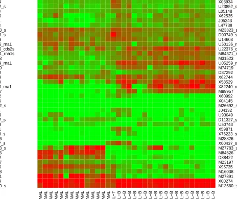
In this paper, we considered the leukemia data as a three-class problem. To compare the classi-fication performance of MPSVM with that of MSVM, the same procedure in Lee and Lee (2003) was used to preprocess the data: (i) thresholding (floor of 100 and ceiling of 16,000), (ii) filtering (exclusion of genes with max/min ≤ 5 and max - min ≤ 500 across the samples), (iii) base 10 logarithmic transformation. The filtering resulted in 3571 genes. After these initial steps, each array was then standardized and F-tests were used to select 40 genes with the largest F-statistics. Figure 6.1 plots the heat maps of the training set and testing set, in which the horizontal rows represent genes, whereas the columns represent samples. The colors depict gene expression values from green (large negative) to red (large positive). For the training set, samples from each class were put together, and hierarchical clustering was used to order the genes so that genes close to each other had similar expression values across the training samples. From Figure 3(a), we can see that for each class, some subset of genes were highly expressed so that the selected 40 genes were very informative in discriminating the three classes. In the heat map (Figure 3(b)) of the testing set, the order of genes was the same as that in the training set, and hierarchical clustering was used to order the testing samples. The expression pattern of testing samples in Figure 3(b) seems to match very well with that of the training samples in Figure 3(a).
Since the sample size was small, the performance of MPSVM and one-versus-rest PSVM was quite robust to the choice of tuning parameters. Using various equally good tuning parameters, no
AML AML AML AML AML AML AML AML AML AML AML
ALL−T ALL−T ALL−T ALL−T ALL−T ALL−T ALL−T ALL−T ALL−B ALL−B ALL−B ALL−B ALL−B ALL−B ALL−B ALL−B ALL−B ALL−B ALL−B ALL−B ALL−B ALL−B ALL−B ALL−B ALL−B ALL−B ALL−B
M13560_s X00274 M27891 M16038 X95735 M23197 D88422 M84526 M27783_s X00437_s M28826 X76223_s X59871 U50743 D11327_s U93049 J04132 M26692_s X04145 X60992 M89957 X82240_rna1 X58529 X62744 D87292 M74719 U05259_rna1 M31523 M84371_rna1s U22376_cds2s U50136_rna1 U14603 D00749_s M23323_s L47738 J05243 X62535 L05148 U23852_s X03934
(a) Heat map of the training set
AML AML AML AML AML AML AML AML AML AML AML AML AML AML
ALL−T ALL−B ALL−B ALL−B ALL−B ALL−B ALL−B ALL−B ALL−B ALL−B ALL−B ALL−B ALL−B ALL−B ALL−B ALL−B ALL−B ALL−B ALL−B ALL−B
M13560_s X00274 M27891 M16038 X95735 M23197 D88422 M84526 M27783_s X00437_s M28826 X76223_s X59871 U50743 D11327_s U93049 J04132 M26692_s X04145 X60992 M89957 X82240_rna1 X58529 X62744 D87292 M74719 U05259_rna1 M31523 M84371_rna1s U22376_cds2s U50136_rna1 U14603 D00749_s M23323_s L47738 J05243 X62535 L05148 U23852_s X03934
(b) Heat map of the testing set
Figure 3. Heat maps of leukemia data.
or one testing sample was misclassified by the MPSVM and the one-versus-rest PSVM. One testing sample was misclassified using the GACV tuning and 0.8 testing sample on average was misclassified using leave-one-out cross-validation tuning by the MSVM (table 1, Lee and Lee (2003)). This demonstrates that the performance of MPSVM is comparable to that the MSVM while MPSVM is much quicker to implement.
6.2. Small round blue cell tumors data. The small round blue cell tumors of children data set was published in Khan et al. (2001). There are four tumor types: neuroblastoma (NB), rhab-domyosarcoma (RMS), non-Hodgkin lymphoma (BL/NHL), and Ewing family of tumors (EWS). The data set contains 2308 genes out of 6567 after some filtering procedure. There are 63 samples (BL: 8, EWS: 23, NB 12, EWS: 23) in the training set and 20 samples (BL: 3, EWS: 6, NB 5, EWS: 20) in the testing set. Similar to the approach for the analysis of the leukemia data, the data were logarithm-transformed and F-tests were used to pre-select 40 genes with the smallest p-values. The testing errors by both MPSVM and one-versus-rest PSVM were 0. This dataset has
been analyzed by the use of many methods (Khan et al. (2001), Lee and Lee (2003), Dudoit et al. (2002), Tibshirani et al. (2002), etc). Nearly all classification methods yield 0 testing errors.
APPENDIX
Proof of Theorem 1: Let fj(x) =βj0+hj(x) with hj ∈ HK for j = 1, . . . , k. Consider the decompositionhj(·) =Pni=1βjiK(xi,·) +ρj(·), whereρj(·) is the element in the RKHS orthogonal to the span of {K(xi,·), i= 1, . . . , n}. By the sum-to-zero constraint, there is
fk(·) =− k−1
X
j=1 βj0−
k−1
X
j=1 n
X
i=1
βjiK(xi,·)− k−1
X
j=1 ρj(·).
By the definition of K, we have< hj(·), K(xi,·)>HK=hj(xi) for i= 1, . . . , n. Thus
fj(xi) = βj0+hj(xi)
= βj0+< hj, K(xi,·)>HK
= βj0+< n
X
i=1
βjiK(xl,·) +ρj(·), K(xi,·)>HK
= βj0+ n
X
i=1
βjiK(xi,xj).
Therefore the data fit functional in (8) does not depend on ρj(·) forj= 1, . . . , k. Furthermore,
khjk2 =k n
X
i=1
βjiK(xi,·)k+kρjk2 for 1≤j≤k−1
and
khkk2 =k k−1
X
j=1 n
X
i=1
βjiK(xi,·)k2+k k−1
X
j=1 ρjk2.
Obviously, the minimizer of (8) does not depend on ρj. This implies equation (9). It remains to show that minimizing (8) subject to Pk
j=1βji = 0 for i = 0, . . . , n is equivalent to minimizing (8) subject to Pk
j=1f(x) = 0 for any x. Let ˆK be the n by n matrix with il entry K(xi,xl). Let fj(·) =βj0+Pni=1βjiK(xi, .) be the minimizer of (8) under the sum-to-zero
constraint for any x. Let β∗j = (βj1, . . . , βjn)0 for j = 1, . . . , k. Define ¯βl = 1/kPkj=1βjl for l= 0, . . . , n and
fj∗(·) =βj∗0+ n
X
i=1
β∗jiK(xi, .) = βj0−β¯0+ n
X
i=1
βji−β¯iK(xi, .).
Then f∗
j(·) =fj(·) sincePkj=1fj(·)≡0. However, k
X
j=1
kh∗jk2+β∗j02
= k
X
j=1
β∗j0Kβˆ ∗j +βj20−kβ¯02−1/k
k
X
j=1 β∗j
0 ˆ K k X j=1 β∗j
≤ k X j=1
β∗j0Kβˆ ∗j +βj20= k
X
j=1
khjk2+βj20
.
The equality has to hold sincefj is the global minimizer. This implies ¯β0 = 0 and
Pk
j=1β∗j
0
ˆ KPk
j=1β∗j
= 0. When ˆK is positive definite,Pk
j=1βji = 0 fori= 0, . . . , n. On the contrary, let fj(.) = βj0+Pni=1βjiK(xi, .) be the minimizer of (8) that satisfies Pkj=1βji = 0 for i= 0, . . . , n. Let β∗j = (βj1, . . . , βjn)0 forj= 1, . . . , k. Thus ˆK
Pk
j=1β∗j
= 0 and
0 = k X j=1 β∗j
0 ˆ K k X j=1 β∗j
= k X j=1 n X i=1
βjiK(xi, .)
2 .
It means thatPk
j=1
Pn
i=1βjiK(xi,x) = 0 and hencePkj=1fj(x) = 0 for any x. Proof of theorem 2: SinceE
(f(X)−Y)0W(Y)(f(X)−Y)
=E E
(f(X)−Y)0W(Y)(f(X)−
Y)X
, we can minimizeE
(f(X)−Y)0W(Y)(f(X)−Y)
by minimizingE
(f(X)−Y)0W(Y)(f(X)− Y)X=x
for everyx. Note that cjl = 0 ifj =l, then
Qx(f) = E
(f(X)−Y)0W(Y)(f(X)−Y) X=x
= k X j=1 " k X l=1 cjl
fl(x) + 1 k−1
2#
pj(x)
= k X j=1 " k X l=1
cljpl(x)
#
fj(x) + 1 k−1
2
= k
X
j=1 τj(x)
fj(x) + 1 k−1
2
,
where τj(x) = Pkl=1cljpl(x). Consider minimizing Qx(f) subject to Pkj=1fj(x) = 0. Using the Lagrange multiplier γ >0, we get
Ax(f) = k
X
j=1 τj(x)
fj(x) + 1 k−1
2
−γ k
X
j=1 fj(x).
Then for eachj = 1, . . . , k, we have
∂Ax ∂fj
= 2τj
fj + 1 k−1
−γ = 0 →fj = γ 2τj −
1 k−1.
Since Pk
j=1fj = 0, we have
γ = 2k k−1.
1
Pk
j=1 τ1j .
The solution is given by
(23) fj =
k k−1
1 τj
Pk
l=1τ1l −k 1
−1.
Thus arg maxj=1,...,kfj(x) = arg minj=1,...,kτj(x) = arg minj=1,...,kPkl=1cljpl(x).
References
Agarwal, D. K.(2002). Shrinkage estimator generalizations of proximal support vector machines.
In Proceedings of the 8th ACM SIGKDD International Conference on Knowledge Discovery and Data Mining. ACM Press.
Aronszajn, N.(1950). Theory of reproducing kernels. Transactions of the American Mathematical
Society 68 337–404.
Boser, B. E., Guyon, I. M. and Vapnik, V. (1992). A training algorithm for optimal margin
classifiers. In5th Annual ACM Workshop on Computational Learning Theory (D. Haussler, ed.). ACM Press, Pittsburgh, PA.
Burges, C. J. C. (1998). A tutorial on support vector machines for pattern recognition. Data
Cox, D.andO’Sullivan, F.(1990). Asymptotic analysis of penalized likelihood type estimators. Annals of statistics 181676–1695.
Cristianini, N. and Shawe-Taylor, J. (2000). An Introduction to Support Vector Machines.
Cambridge University Press.
Dudoit, S., Fridlyand, J. and Speed, T. (2002). Comparison of discrimination methods for
the classification of tumors using gene expression data. Journal of the American Statistical Association 9777–87.
Fung, G. and Mangasarian, O. L. (2001a). Multicategory proximal support vector machine
classifiers. Machine Learning, in press.
Fung, G. and Mangasarian, O. L. (2001b). Proximal support vector machine classifiers. In
Proceedings of the 7th ACM Conference on Knowledge Discovery and Data Mining. ACM press.
Girosi, F. (1998). An equivalence between sparse approximation and support vector machines.
Neural Computation 101455–1480.
Golub, T., Slonim, D., Tamayo, P., Huard, C., Gaasenbeek, M., Mesirov, J., Coller,
H.,Loh, M., Downing, J.,Caligiuri, M.,Bloomfield, C.and Lander, E.(1999).
Molec-ular classification of cancer: class discovery and class prediction by gene expression monitoring. Science 286531–537.
Khan, J., Wei, J., Ringner, M., Saal, L., Ladanyi, M., Westermann, F., Berthold, F.,
Schwab, M., Antonescu, C., Peterson, C. and Meltzer, P. (2001). Classification and
diagnostic prediction of cancers using gene expression profiling and artificial neural networks. Nature Medicine 7 673–679.
Kimeldorf, G.andWahba, G.(1971). Some results on Tchebycheffian spline functions. Journal
of Mathematical Analysis and Applications 3382–95.
Lee, Y. and Lee, C. (2003). Classification of multiple cancer types by multicategory support
Lee, Y., Lin, Y. and Wahba, G. (2004). Multicategory support vector machines, theory, and application to the classification of microarray data and satellite radiance data. Journal of the American Statistical Association 9967–81.
Lin, Y. (2002). Support vector machines and the Bayes rule in classification. Data Mining and
Knowledge Discovery 6 259–275.
Lin, Y.,Lee, Y.andWahba, G.(2002). Support vector machines for classification in nonstandard
situations. Machine Learning 46191–202.
Nguyen, D. V. and Rocke, D. M. (2002a). Multi-class cancer classification via partial least
squares with gene expression profiles. Bioinformatics 18 1216–1226.
Nguyen, D. V. and Rocke, D. M. (2002b). Tumor classification by partial least squares using
microarray gene expression data. Bioinformatics 1839–50.
Poggio, T.and Girosi, F.(1998). A sparse representation for functional approximation. Neural
Computation 101445–1454.
Suykens, J. A. K., Van Gestel, T., De Brabanter, J., De Moor, B. and Vandewalle,
J.(2002). Least Squares Support Vector Machines. World Scientific, Singapore.
Suykens, J. A. K.andVandewalle, J.(1999). Least squares support vector machine classifiers.
Neural Processing Letters 9(3)293–300.
Tibshirani, R.,Hastie, T., Narasimhan, B.andChu, G.(2002). Diagnosis of multiple cancer
types by shrunken centroids of gene expression. Proceedings of the National Academy of Sciences USA996567–6572.
Van Gestel, T., Suykens, J. A. K., Lanckriet, G., Lambrechts, A., De Moor, B. and
Vandewalle, J. (2002a). Bayesian framework for least-squares support vector machine
clas-sifiers, Gaussian processes and kernel Fisher discriminant analysis. Neural Computation 15(5) 1115–1148.
Van Gestel, T., Suykens, J. A. K., Lanckriet, G., Lambrechts, A., De Moor, B.
and Vandewalle, J. (2002b). Multiclass LS-SVMs: moderated outputs and coding-decoding
schemes. Neural Processing Letters 15(1)45–58.
Vapnik, V. N.(1998). Statistical Learning Theory. John Wiley, New-York.
Wahba, G.(1990). Spline Models for Observational Data. CBMS-NSF Regional Conference Series
in Applied Mathematics, 59, SIAM, Philadelphia, Pennsylvania.
Wahba, G. (1999). Support vector machines, reproducing kernel Hilbert spaces and the
random-ized GACV. InAdvances in Kernel Methods: Support Vector Learning (B. Scholkopt, C. Burges and A. Smola, eds.). MIT Press.
West, M.(2003). Bayesian factor regression models in the “large p, small n” paradigm. Bayesian
Statistics 7 723–732.
Weston, J.andWatkins, C.(1999). Support vector machines for multiclass pattern recognition.
In Proceedings of the 7th European Symposium On Artificial Neural Networks. Bruges, Belgium.
Department of Statistics, North Carolina State University, Campus Box 8203, Raleigh, NC
27695-8203, USA
E-mail address: [email protected]