A physical multi-body car model using 3-D (screw) bond graphs

(1)

faculteit der

elektrotechniek

Universiteit Twente

A physical multi-body car model using 3-D

(screw) bond graphs

G.R. de Boer

M.Sc. Thesis

Supervisors: Prof. dr. ir. Job van Amerongen

Dr. ir. Stefano Stramigioli

Dr. ir. Edward Holweg

Ir. Vincent Duindam

June 2002

Report Number Report Number

Control Laboratory Dpt. of Electrical Engineering

University of Twente P.O. Box 217

(2)

(3)

Acknowledgements

(4)

(5)

Summary

The goal of the project was to realize an infrastructure of a car in 20-SIM using (screw) bond graphs. Bond graph description is an energy based means of modeling physical systems. This model can be used for investigation of the X-by-wire concept and independent wheel steering. Enquiry into the basic features of a car provided for the necessary insight in the course of development of the car. Rigid bodies have been used to describe the most significant masses of the car. These are interconnected as so-called kinematic pairs. Within these kinematic pair connections, constraints are used to restrict the separate elements of the car to specific motions only.

Setting the steering angle has been realized with the use of the Ackermann algorithm, which distinguishes between the track (and thus also the radius of curving) of the two front wheels. For more realistic steering behavior, the steer-ing axes of both front wheels have been canted slightly, accordsteer-ing to the Ksteer-ingpin and Caster angles in genuine cars. The resulting model is a realistic reflection of a car is obtained.

With the use of Gauss-maps on the surfaces of the tire and the ground, a contact determining algorithm has been developed. The velocity of the contact point of the wheel relative to the contact point of the surface is fed to a buffer returning an oppositely oriented force. Thus a forward propulsion is accom-plished. Monitoring the force in the contact point and switching to coulomb friction behavior in case the force exceeds a set threshold value, enables the modeling of slip behavior. The slip in the horizontal plain has been coupled. Slip in one direction results in a loss of grip in the perpendicular direction as well.

(6)

(7)

Chapter 1

Introduction

The design of a car nowadays involves a multitude of disciplines. Although in the course of time, the emphasis in the design has been extended from mere functional and technical cunning to e.g. aesthetics and originality, the focus of the research in this thesis will be on the former aspect. The report will enquire into the physical behavior of a car, and how to describe it appropriately.

Some other disciplines besides the functional behavior of enabling the driver to move from point A to point B, are safety and comfort. Much research has been performed in the field of airbags, seatbelts and energy dissipating frameworks in order to increase safety. Active driving control systems influencing the power and brake distribution to the tires, such as ABS (Anti-lock Braking System) and ESP (Electronic Stability Program) provide the user with more safety as well.

More comfort nowadays is achieved with systems like active suspensions, adaptive seats, noise reduction in the cockpit and a variety of electronically remote-controlled features for e.g. windshields, mirrors and headlights.

A field of research covering both safety and comfort is the X-by-wire ap-proach. Similar to the fly-by-wire systems in aeroplanes, the goal is to replace all mechanically or hydraulically controlled functions of a car by electronic ac-tuation. This means no more hydraulic brakes, no mechanical gas lever, no steel steering shaft. Electrical control of these functions enable even more fundamen-tal driving control systems.

Hence, steer-by-wire implies that the steering wheel will not be mechanically coupled to the front wheels. the steering wheel will be attached to an electrical actuator to give a force feedback and a sensor to measure the position of the angle set by the driver. On the other hand, the tire angles will be actuated by an electrical motor. In between, there will be a computer which will evaluate the drivers actions and actuate the tires accordingly.

A further step is the possibility to even uncouple the two front wheels and actuate them separately with two electrical drives. This gives the possibility to have different relative turning angels depending on the speed and on the driving situations. A control strategy needs to be found for this independent steering.

(10)

structure of a car should be considered; especially the contact between the tires and the ground. The required model will be developed using (screw) bond graph techniques.

Of course there are quite a few software tools available aiming specifically at car design. Most of these can be categorized as either industrial (CAD) design tools for constructional design or mathematical models for physical descriptions. To the authors knowledge, no car model has yet been developed using screw bond graphs.

Screw bond graphs have been chosen for the modeling because they represent an energy based approach. This approach facilitates energy consistent imple-mentation and it reduces the error proneness of the model. Moreover, screw bond graphs provide for a means of modeling, independent of the physical do-main of the model. They can be applied whether a specific part of the model belongs to the electrical, mechanical or chemical domain. This means that all model parts (e.g. engine, suspension, steering controller) can be modelled in the same structure.

For the bond graph design, 20-SIM has been chosen. This is a very apt modeling tool, combining powerful model calculation features with useful visu-alization features. Most admirable is its DirectX 3D environment, allowing an instant 3D display of the model.

(11)

Chapter 2

Bond Graphs

In the history of design and analysis of complex systems, the need for accurate models of these systems has increased. Modeling based on energy flows has proven to be very rewarding. When connecting two systems, energy can be exchanged between them. Bond graphs are a means of describing an intercon-nection of systems on such an energy flow-basis, independent of the physical domain of the model. They were first introduced by Paynter (Paynter, 1961).

Bond graphs are built up as follows. The positive orientation of the power is indicated by the direction of a half arrow, called a bond (see Figure 2.1). This

system1

system2

system3

Figure 2.1: a bond and a multi bond

figure also shows a so-called multi bond. This is a bond which transports energy flows with more than one dimension (e.g. for a movement along two axes).

A bond actually consists of two factors, thegeneralized flow and the gener-alized effort. For any of the physical domains in the model, a bond is available which consists of an appropriate version of these two variables. So the powerP, represented by the bond graph, can be represented by the product of its effort

eand flowf.

P =e·f

In the electrical domain the effort and flow are respectively the voltage U

andcurrent I. In the mechanical domain they can be recognized as theforce F

andvelocity v in case of translation, and as thetorque T andangular velocity

ω in case of rotation.

2.1

Causality

(12)

directed in the opposite direction of the effort, so in the figure, the flow is an output of system 2.

Sometimes the causality can be freely chosen, but quite often an element has a preferred or even a fixed causality. When modeling, these restrictions have to be well considered. Neglecting them could result in undesired simulation results or even an inability of 20-SIM to evaluate the model.

2.2

Bond Graph Elements

20-sim provides for many basic elements to create an actual model. This section gives a short description of the elements used in the model of the car, and how they can and should be used. We can distinguish between sources,dissipators,

buffers,transformers,gyrators andjunctions.

2.2.1

Sources

Source elements (S-elements) are power generating elements. One can choose to use a Source of Effort Se or a Source of Flow Sf. Other possibilities are the Modulated Source of EffortM Seand the Modulated Source of FlowM Sf. These sources have the possibility of being controlled by an external signal. The causality of these elements is fixed, soSeandM Seelements are effort-out and

Sf andM Sf are flow-out (or effort-in).

2.2.2

Dissipators

Dissipators are elements that can dissipate energy. In 20-sim its symbol is an

R. The R-element can be used to model resistance or friction. The causality of the R-element is indifferent. The dissipator can be both effort-in as flow-in.

2.2.3

Buffers

Buffers are elements that can store energy. We can distinguish between two types: I-elements and C-elements. The linear I-element relates the flow and the integrated effortp. The energy (E(q))function of the I-buffer is

EI(p) = 1 2Ip

2

with p=

Z

edt+p(0)

f =∂E

∂p =

1

I p

The linear C-element on the other hand relates the effort and the integrated flowq.

EC(q) = 1 2Cq

2

with q=

Z

fdt+q(0)

e=∂E

∂q

1

C q

(13)

2.2 Bond Graph Elements 13

2.2.4

Transformers

Ideal transformers are depicted by a TF-element. It is a power-continuous multi port element, relating both the efforts and the flows of the input and output. The effort relation is described as follows.

ein=n eout

The demand of power continuity appoints the constitutive relation of the flow.

fout=n fin

Similar to the modulated sources, these TF-elements also come in a modulated version. These elements are depicted asM T F. In an MTF, the transformation factornis set externally and may vary in time.

Figure 2.2: transformer element

2.2.5

Gyrators

AGY-element is also a power-continuous multi port element, and it relates the input effort to the output flow and vice versa. So these are its constitutive relations.

ein=g fout Power continuity requires the second relation to be:

eout =g fout

Similar to the transformer element, also a modulated version of the gyrator,

M GY, can be applied. In these elements, the gyration factor g is applied externally and can have a varying value.

Figure 2.3: gyrator element

2.2.6

Junctions

To be able to manufacture any structure whatsoever with these elements, con-nection elements are needed. These elements need more than two ports. Two junctions can be recognized, the 0−junctionand the 1−junction. They have to answer the following two requirements.

(14)

Port symmetry implying that the constitutive relations of the ports are ex-changeable. One can develop these relations to the effort of flow of any of the connected elements.

The 0-junction behaves analog to Kirchhoff ’s junction rule in the electrical domain, so the sum of all flows entering and leaving the junction is equal to zero and all the efforts have the same value. For example, aparallel connection

in the electrical domain is modeled in this fashion. In the 1-junction on the other hand, the sum of all the efforts in the junction is zero and all the flows are equal, just like inKirchhoff ’s loop rule for the electrical domain. An example of such a junction in the electrical domain is aseries connection.

2.3

Screw Bond Graphs

Before proceeding to the model, the concept of screw bond graphs has to be reviewed. Consider a 3 dimensional Euclidean space,E(3). We can describe the position and orientation of every body by an element of the Special Euclidean group SE(3). Now consider two right-handed coordinate frames within this space, Ψi and Ψj. A general change of Cartesian coordinates inE(3) from Ψi to Ψj can be expressed with a homogeneous matrix of the form:

H_ij =

Rj_i pj_i OT

3 1

(2.1)

whereRi

jis a rotation matrix (element of the special orthonormal groupSO(3)) and pi

j is a vector inR

3

. Hi

j denotes the change of coordinates from a right-handed coordinate frame Ψjto another right-handed coordinate frame Ψi. Thus it can be used to for example describe the position and orientation of a body (with attached coordinate frame Ψj) relative to a reference (inertial) coordinate frame (Ψi).

The instantaneous velocity of a body i with frame Ψi relative to a body j with frame Ψj can be represented by atwist Tik,j, with

T_ik,j=

ωk,j_i vk,j_i

(2.2)

where ωk,j_i denotes the angular velocity of body irelative to bodyj expressed in coordinate frame Ψk. On the other hand, vik,j denotes the instantaneous lateral velocity (relative to frame Ψj) of the point fixed in frame Ψi that passes through the origin of frame Ψk. A twist can be regarded as the derivative of a homogeneous matrix in the following way:

˜

T_ij,j :=

˜

ωj,j_i v_ij,j

0 0

= ˙H_ijHi j

where ˜ω is the skew-symmetric matrix equivalent to (ω× ·). Similar to the homogeneous matrix, describing the change of coordinates for two coordinate frames, an Adjoint matrix can be used to change the coordinate frame in which the twist is expressed. We define the adjoint operatorAdHk

j as

T_ik,j=Ad_Hk jT j,j i = Rk j 0 ˜ pk

jRki Rkj

(15)

2.3 Screw Bond Graphs 15

(Duindam and Stramigioli, 2002b)

Chasles’ decomposition theorem states that any element of SE(3) can be described as a pure instantaneous rotation around an axis plus a pure instanta-neous translation along the same axis:

ω v

| {z }

twist

=kωk

ˆ

ω r ∧ ωˆ

| {z }

rotation +λ 0 ˆ ω

| {z }

translation

(2.3)

whereω=kωkωˆandλis called thepitch. Examination of this formula with reference to figure 2.4 shows thatv is the velocity of an imaginary point passing through the origin of the coordinate system in which the twist is expressed and moving together with the object. The twist can be associated with a geometrical line, namely the line passing throughrand spanned byω, which is left invariant by the rotation.

Figure 2.4: intuition of a twist

More information on twists can be found e.g. in (Murray, Li and Sastry, 1994; Stramigioli, 2001).

We can also define a wrench Wk

i (the dual of a twist), which describes the generalized forces acting on bodyiand expressed in frame Ψk, as

Wik =

τk i Fk i (2.4)

where Fk

i denotes the linear force andτik the momentum, acting on the point in the origin of frame Ψk. The dual product of a twist and a wrench (when expressed in the same coordinate frame) is equal to a power flow.

(16)

onSE(3), i.e. the space of wrenches) can be split as a sum of two terms:

m f

| {z }

wrench =

r∧f f

| {z }

f orce +λ

f

0

| {z }

momentum

(2.5)

Analogue to the twist, Figure 2.5 shows how a wrench can be visualized. In

Figure 2.5: intuition of a wrench

Figure 2.5, the first element of equation 2.5 is representing a pure force applied along the line passing through r. The second is instead a pure momentum which does not need to be associated to a finite line, but to an in infinite line which is again the polar of the line representing the pure force. (Stramigioli and Bruyninckx, 2001)

(17)

Chapter 3

The Car

Before diving headfirst into the modeling steps and development trajectory, some key features of a car need to be mentioned. This chapter will specify basic attributes of a modern car and touch some choices that have been made in the design of the model. Using the characterization of these features and subsystems, the model can be iteratively enhanced, adding more subsystems and features in every step.

In order to study a car, it is necessary to specify one or more coordinate systems to measure the position of the vehicle. First of all there is an Earth-fixed coordinate system Ψ0. Within this analysis this frame will be considered

inertial. Next, a body-fixed frame has to be assigned to the car body, Ψcar. The z-axis is chosen in the forward driving direction. The y-axis is vertically upwards and the x-axis is chosen such that a right hand coordinate system is realized. Figure 3.1 shows this configuration. Each element (or group of elements) in the

Figure 3.1: the different motions in the vehicle-fixed frame

(18)

in a separate coordinate frame (e.g. the wheels, axles and bearings).

Besides translation along the axes of its frame, the car body can rotate around these three axes. Figure 3.1 also shows these motions and the terminol-ogy that will be used (Rahnejat, 1998), (Dixon, 1991).

With these six Degrees Of Freedom (DOF) all elements which constitute a screw motion are known.

The car can be divided in several subsystems, each representing an elemen-tary function of a car. These are the wheels (and axes), the suspension and the steering. First of all we will have a closer look at the suspension.

3.1

The Suspension

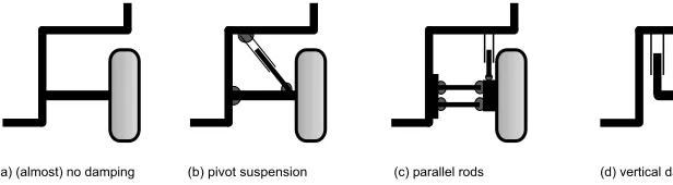
Suspensions come in various types, depending on the desired behavior. A first selection is made when the desire for independent springs is uttered. This rules out all variations of torsion suspension, which damp both wheels on either side of an axle. When the requirement for separate suspensions is added, only single wheel suspensions remain. Figure 3.2 shows some variations of single

Figure 3.2: some (simple) suspension types

wheel suspensions. As can be seen, Figure 3.2 (a) only damps vertical motions slightly because of the finite stiffness of the axle. Figure 3.2 (b) damps the vertical motions using an axle connected to a hinge point. The wheel describes a circular rather than a vertical motion around this point. This configuration is not commonly used anymore. Item (c) of Figure 3.2 uses two parallel rods to enable an almost vertical motion for the wheel. Several wishbone suspension types are based on this concept. This is the most realistic variation in the figure. Finally, Figure 3.2 (d) shows a truly vertical motion, albeit not realistic in construction. However, the simulator does not care for realism very much (in this respect), and this representation does meet our need for vertical damping in an incomplex way. That is why the suspension in the final model resembles type (d).

Constraining a rigid body to certain motions only, can give rise to some difficulties, since some screw motions are coupled. For a rigid body, circular motions are mechanically coupled to translational motions. So when a rotation as well as a translation is desired, a third, undesired motion can occur. This problem can be solved by projecting the motion of the body onto the feasi-ble directions and ignoring the forces in the constrained direction, using the

(19)

3.2 The Wheel 19

performs one particular movement. In the model, the latter solution has been applied by defining a bearing. This way, the axle can be constricted to sole rotations and the bearing to mere vertical translations.

It be noted that of course in real cars, the wheel is not only connected to the car body by an axle, but e.g. by an above mentioned wishbone-type suspension. A separate axle accounts for the rotation. But as we have chosen the simple suspension type (d) and we want to avoid the coupled motions, the bearing is needed. Figure 3.3 shows a view of the model in which this bearing is clearly visible. As can be seen in Figure 3.3, the axle of the car goes right through this

Figure 3.3: the vertical suspension and bearing on the car axle

bearing. The bearing is connected to the axle on a fixed position, and can only translate vertically. The axle can now rotate around the x-axis trouble-free.

3.2

The Wheel

The wheels play a significant role in the model, since they enable the contact to the surface. To provide the reader with an elementary insight in the processes involved in this contact, some fundamental behavioral aspects are reviewed.

In vehicle handling analysis, the tires are generally represented by empirical models; these are non-phenomenological, that is, the tire behavior is not de-rived from the material properties and structure of the tire. The material of a tire is a multi-layered, non-uniform, anisotropic, cord-rubber composite. So to understand tire behavior, there is a pressing need for simplification.

(20)

implemented (Figure 3.4 (a)). At the contact point, forces are exerted from the

Figure 3.4: representations of wheel contact

wheel to the ground surface for vehicle support, guidance and maneuvers. These characteristics are all influenced by the operating parameters of a tire such as its inflation pressure, its rolling velocity and its size and shape (of Transportation, 1985). When implementing a contact model, these parameters have to be taken into account.

Surface parameters influence the driving behavior of the car to a great extent as well. Rough tarmac surfaces will feature more grip for the tires than e.g. wet asphalt or a dirt road. However, also in this respect the need for accuracy is not very urgent. We mainly want to distinguish between slippery and not-so-slippery surfaces. This can just as well be simulated by varying the friction parameters of the tire model. With these considerations a sufficient tire contact model can be constructed.

3.3

The Steering

The final basic feature of the car is the ability to steer. In almost all cars, this happens by rotating the front wheels around the vertical axis of the wheel. Setting both wheels to a certain equal angle, and thrusting the car forward, will make the car follow a curved course. This way the car can move freely on a plain, and one can maneuver the car to any desired location. However, true cars do not steer both wheels by an equal amount. Besides, steering does not actually happen by rotating the wheels around a vertical but rather around a slightly slanted steer axis. The following sections show how these attributes can be implemented for the car model to steer in a realistic fashion.

3.3.1

Ackermann Steering

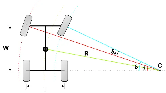
When the car is steering in a low-speed situation, i.e. the side slip of the front wheels can be neglected, the trail the inner tires cover is not identical to the track of the outer tires. The inner tires follow a circle with a smaller radius than the outer tires. This means the front wheels have to be set to a different angle too, corresponding to the radii of their trajectories. Disregarding this property will eventuate in excessive tire scrub and poor steering behavior. Figure 3.5 displays how these dissimilar trails are to be interpreted.

(21)

3.3 The Steering 21

Figure 3.5: the Ackermann steering concept

In the figure, R depicts the radius of the curve measured from the car center, C is the center of rotation, T is the track width and W is the wheel base of the car. The following relations can be derived.

δo=tan−

1 W

R+T

2

!

δi=tan−

1 W

R−T

2

!

(3.1)

Whereδo is the angle of the outer tire andδi the angle of the inner tire. The Ackermann angleδA is the difference between these angles.

δA=δi−δo

Now, when the radius of the curve (R) is set to the desired value using the steer angle as in

R= W heelBase 2·sin−1₍_SteerAngle₎

both the inner (δi) and outer (δo) angle can be determined. The radius of the curve has been determined from the center of the wheelbase (W heelBase/2).

3.3.2

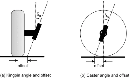
Kingpin and Caster

(22)

Figure 3.6: the distinction between the Kingpin and the Caster angle

Figure 3.7: the effect of the Kingpin and Caster angle

The Caster offset, together with the Kingpin angle, affect the camber angle of the tire (the tilt of the tire around the z-axis) in a steering motion. Figure 3.7 shows a picture from the 3D model in which the effect of Kingpin and Caster angle are distinctly visible. To increase clarity, the coordinate frames of the front tires have been displayed as well. The vertical axes of the front wheels show different inclinations, due to the Ackermann steering concept (which is also visible by the different directions of the z-axes of the tires).

The inner tire which, due to the Ackermann geometry, has the greater steer-ing angle, also exhibits more camber. Both these angles and offsets influence the handling of the car, especially in small-radius corners. In actual cars, such steering behavior is defined by a pair of ball joints, rather than an inclined steer axle. The resulting steering motion however remains similar.

(23)

Chapter 4

The Model

Now we have arrived at the main chapter of this thesis. This chapter will elab-orate on the modeling steps that were implemented to obtain a fully functional model of a car. The first endeavor is familiarizing with screws and constraints. This will be done using a wheel and axle configuration as described in Section 4.1. With this knowledge, iteration steps can be taken to gradually increase the complexity and veracity of the model. Each of the sections will cover partial enhancements until the desired functionality is reached.

4.1

Wheel and Axle

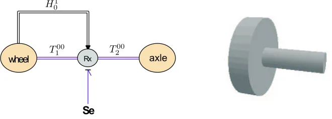
We commence the research with a simple wheel and axle construction. They are connected by a kinematic pair, and in the connection all motions but a rotation around the longitudinal axis of the axle are constrained. When an wrench is imposed on the first element of the screw bond in the kinematic connection (the rotation around the x-axis, as can be seen in equation 2.4), the wheel and the axle start rotating in opposite direction. This behavior is consistent with the physical law of conservation of momentum. Figure 4.1 shows the iconic representation of the implementation of this subsystem in 20-SIM.

wheel axle

Se

Rx

PSfrag replacements

H1 0

T00

1 T

00 2

Figure 4.1: the iconic and 3D of a wheel and axle

(24)

but rotations around the x-axis. The right hand side of the figure shows a depic-tion of the 3-D representadepic-tion of this bond graph model. The 3-D environment has been frequently employed for an intuitive verification of the model.

In this elemental subsystem, some essential submodels have been applied. Since the will turn up in several other regions of the model as well, they are briefly explicated in the following sections.

4.1.1

Rigid Bodies

Thewheelandaxissubmodel have been based on the so-called rigid body model. This section will give a brief explanation of these submodels.

Since we are modeling in 3D, all objects in the model have to be able to move with 6 DOF. Hence, a model of a rigid body is needed that comprehends all the six elements that draw up the 3D screw motions. Moreover, dynamical aspects like acceleration of gravity, moments of inertia and coriolis forces have to be implemented.

We start by taking the momentum of a point mass m p=mv

where p is the impulse or momentum andv is the velocity of the mass. This equation is known as Eulers equation. By taking the derivative of both sides, we obtainNewtons second law of dynamics, which is defined as

F = ˙p=mv˙+ ˙mv

where ˙v is the acceleration of the point mass. For most cases, where the mass has a constant value, the formula simplifies to

F =p=mv˙

Including the rotational domain as well, we take the momentum for the rota-tional inertiaJ defined by

pr=Jω

where pr is the angular impulse or angular momentum and ω is the angular velocity. Again we take the derivative of both sides to get

˙

pr= ˙Jω+Jω˙

where ˙ωis the angular acceleration. ˙J is zero for most cases, so that we get the simplified form of

˙

pr=Jω˙

Noting that ˙p is equal to the forceF and ˙pr is equal to the torque τ, we can generalizeEulers equation for a rigid body by

P =IT (4.1)

whereP = [pT

rpT]T is the generalized momentum andT = [ωTvT]T is the twist.

Iis a 6x6 inertia matrix. Finding or calculating this matrix can be simplified by using theprincipal inertia frame. For any rigid body, a special frame Ψkcan be found, that is placed in the center of gravity, and oriented such, that

Ik,i=

Ji 0 0 miI

(25)

4.1 Wheel and Axle 25

where

Ji=

 

jx 0 0 0 jy 0 0 0 jz

 

I can then be found by

Ii₌_AdT Hk

iI

k,i_Ad Hk

i.

When we differentiate Eq. 4.1 on both sides we obtain the generalized formula of Newtons law which is defined in an inertial frame as

˙

P =W (4.2)

where ˙P is the time derivative of the momentum of the rigid body, andWT ₌ [τT_FT_{] is the applied wrench. If we use the indices to indicate the frames, we} get ˙P of bodyirelative to frame Ψ0 defined in frame Ψ0

˙

Pi,0

o =W

0,i

0

To be able to make use of the principle inertia, we transform the formula from the reference frame ψ0 to the body frame ψ_i. After some manipulations, we

arrive at the power balance for a rigid body:

˙

PiT_ii,0

| {z }

1

=Piad_Ti,0

i T

i,0

i

| {z }

2

+WiT_ii,0

| {z }

3

(4.3)

In Eq. 4.3, the first term on the left (1) is the stored energy. The second term on the right (3) is the supplied energy. We see that an extra term has appeared (2), that always has a power value of zero, due to the structure of

ad_Ti,0

i . Nevertheless, this term must not be omitted, and can be found directly

in the used 20-SIM models. The extra term is a consequence of the position of our reference frame. In Eq. 4.2 the momentum is defined with respect to the reference frame of the observer. In Eq. 4.3 the reference frame is the body frame itself.

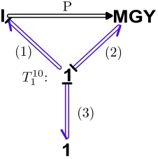
To model this in bonds graphs we get a model as depicted in Fig. 4.2. We can see that the model is a direct result of the above equation. The dimension of one multi-bond is 6. We would like to apply wrenches to the rigid body, that are defined in the reference frame of the rigid body. We need to apply a

I

MGY

1

PSfrag replacements (1) (2)

(3) P

T10 1 :

(26)

coordinate change in order to do this. We get

T11,0=AdH1 0T

0,0 1

whereAdH1

0 is the adjoint mapping from frameψ0 to frame ψ1. This

transfor-mation is realized by an MTF-element, with an extra modulation input signal

H1

0 that changes the transformation ratio. H 1

0 can be calculated according to

H1 0(t) =

Z t

0

˙

H1 0(t) +H

1 0(0)

where

˙

H1 0 = ˜T

1_,1 0 H 1 0 and H1 0(0)

is the initial configuration.

To calculate the integral we must use an initial H-matrix (Hinit), which can be chosen by looking at the starting configuration. The gravity force (G) is implemented in the same submodel causing an externally applied wrench, which is defined in the reference frame (Cs). We findτ, caused by the gravity force, by taking the cross-product ofG and the displacement vectorp, which is part of the homogeneous matrix we have calculated above. A complete model for a

I

MGY

1

Cs

MTF

1

PSfrag replacementsH1 0

T10 1 :

T00 1

:AdH1 0

T00 1

Figure 4.3: 3D Rigid Body

three dimensional rigid body that can be used for screw bond graph modelling is obtained. To define the screw motion, two coordinate frames are used. The reference frame Ψ0 and the body frame Ψ1are located at the center of gravity.

We write the twist as T0

i. This is the rigid body model as applied in the car model (Keukens, 2001).

4.1.2

Constraints

(27)

4.1 Wheel and Axle 27

PowerIn

0

PowerOut

1

MTF

1

Constraint

wheel Rx axle

PSfrag replacements

T00

1 T

00 2

:T02 1

:T12 1

:AdH1 0

H1 0

Figure 4.4: the insides of the kinematic pair connection

constraints on the motions are defined. This is done in the following manner. Figure 4.4 shows the transformations applied to the screw bond graphs. The bond graph model can be interpreted as follows. The top of the structure displays two 1-junctions, representing the twists of body one (the wheel) and body two (theaxle), relative to and represented in the frame Ψ0(the Earth-fixed

frame). The constraints concern motions in the frames of the bodies rather than in the Earth-fixed frame. So before we can effectively impose constraints on this system, we have to transform the screw bonds in such a way that the relative velocity of the bodies is represented in either one of their coordinate frames. As can be seen in the figure, the bonds are transformed so that body one is related to body two, and represented in the coordinate frame of body one (T12

1 ). The

twist (T02

1 ) of body one, relative to body two is obtained simply by subtracting

them using a 0-junction (the sum of all flows in a 0-junction is zero). Finally, using the H-matrix from body one to construct an Adjoint matrix (AdH1

0) to

change the frame of representation gives the desired result.

(28)

With this simple analysis of a wheel and axle, an essential strategy has been drafted for the actual car model.

4.2

The Car Body

Finally we have arrived at the stadium where the real car model will be drawn up. The core of the car body is a rigid body like any other. It will only differ from rigid bodies for e.g. the wheels or bearings in mass and inertia, as can be seen in Chapter 5. The pith of the modeling are the connections and constraints with the other rigid bodies.

The car model will be built up stepwise, beginning with the wheels from the previous section. The car needs four of these subsystems. Each of these wheels-axle systems has to be connected to the car body with a suspension. Eventually, a torque has to be imposed on the wheels for the propulsion, and the steering has to be implemented.

4.2.1

The Suspension

The suspension requires a damped vertical motion as mentioned in section 3.1. This means that the kinematic pair of the wheel and axle have to be kinemati-cally connected to the car body and constrained to pure vertical motions.

Figure 4.5 shows this construction for one wheel. The icon of a wheel and axle contains the subsystem of section 4.1. The restriction to vertical movements (Ty) is done in a similar fashion as the rotation of the wheel. It can be seen that the bearing discussed in section 3.1 comes into use here. The iconic depiction of

CarBody

Bearing Ty

Figure 4.5: the bond graph model of the suspension

(29)

4.3 The Steering 29

F = 1

2·k2 (x+

p

(x−s/2)2_{+ (}_ep_·_s₎2₊_x_{− · · ·}

· · · −p(−x−s/2)2_{+ (}_ep_·_s₎2_{) +}_k₁_·_x₊_d_·_v _(4.4)

Where

F = Force

k1 = stiffness in the nominal region

k2 = stiffness outside the nominal region

s= interval of the play i.e. the suspension region

d= damping, equal tod1 within the nominal region andd2 outside the region

ep= ”sharpness” of the transition region

v = the vertical velocity

For a more detailed description of the suspension, refer to the Appendix.

4.2.2

Four Wheels and a Car Body

Little exertion is needed to extend the model to a complete car body with four wheels and suspensions. Figure 4.6 shows the schematic depiction of the car and the wheels, where the car body and wheels are expanded to display their contents. Although one is tempted to read the tiny submodels and signals, this figure only serves the purpose of showing the general structure of the model. The arrows show the direction of development from the center rigid body of the car to the wheels. The dotted outlines indicate where the car body part of the iconic diagram on top of the figure is to be found in the bond graph model.

As can be seen, the front wheels differ from the original wheel axle system of section 4.1. This is necessary to enable steering motions in the front wheels. The following section will discuss how the steering has been realized.

4.3

The Steering

Analog to separating rotational and translational movements to prevent inter-ference, a new rigid body has to be defined which is confined to steering motions (rotations around the vertical axis). This body can be recognized in 4.6 as the

Rotator. A kinematic connection (Ry) restricts its motions. As we know now, this rotation does not occur around a pure vertical axis, but rather a slanted steering axis. This means that within Ry, apart from the regular transforma-tion in a kinematic connectransforma-tion, an additransforma-tional transformatransforma-tion has to take place. This way, the constraints are imposed on a frame with a Kingpin and Caster inclination relative to the original frame.

An additionalTFelement has been implemented in the standard kinematic connectionRybetween theAxisand Rotator, tilting the body fixed frame by a Kingpin and Caster angle (4.5).

T_KCKC,2=AdHKC

1 ·T

1,2

1 with AdHKC

1 =Adjoint(H

KC

(30)

The

Mo

del

H RearRight HRearRight

RearLeft

FrontLeft FrontRight

HRearLeft

HFrontLeft HFrontRight

Rx

CarBody BearingRR

Ty Ty

BearingRL

BearingFR BearingFL

C

Rx

C

SteerAngle

CarWheel Rx Ry CarAxis

PID

Rotator

Contact WheelAxis

H

SteerAngle

CarWheel

Rx Ry

CarAxis

PID

Rotator

WheelAxis

Figure

4.6:

the

complete

car

b

o

dy

b

ond

(31)

4.4 The Driving 31

HKC

1 =HK·(HC)T =

 

cosK −sinK 0 sinK cosK 0

0 0 1

 

 

1 0 0

0 cosC −sinC

0 sinC cosC

 

T (4.5)

WithK the Kingpin angle andC the Caster angle.

A steering angle is set by implying a force on the kinematic connection be-tween the axle rigid body and the rotator body. To be able to set the steer angle to a desired value, a PID controller has been implemented. This controller feeds a force to the kinematic connection in proportion to the difference between the desired angle and the actual angle. The rigid bodies only contain information of the position and orientation of the bodies relative to the Earth-fixed frame. Hence, a relative H-matrix has to be constructed, relating the position orien-tation of the Rotator to the Axis or vice versa. This can be realized with the following straightforward operation.

Hrelative= (HRotator)T·HAxle

Figure 4.7 shows how the controller has been implemented. Chapter 5 reports on how the control parameters have been determined. The front wheels have

SteerAngle

MSe

SteeringForce

Abs to Rel

PID PSfrag replacements steerangle steeringf orce H0 1 H 0 2

Figure 4.7: the PID controller implemented for steering

separate controllers, their setpoints following the Ackermann algorithm. A spe-cial submodel has been created which converts a steering angle to a separate Ackermann angle for each wheel. For a more detailed description on the steering as implemented in 20-SIM, refer to the Appendix.

4.4

The Driving

The model has been designed to allow both front, rear and four wheel driving. A signal generator provides for the speed the wheels have to follow. A PID controller ensures that this speed trajectory is realized, within a small error tolerance.

(32)

However, in 20-SIM we are not limited to the use of one ’engine’ (i.e. Effort Source). We can simply implement several sources. Moreover, the connection between the sources and the wheels is not locked like in actual cars. Applying an equal torque on e.g. both rear wheels does not confine the wheels to equal rotational speeds. The sources are ideal, which means that whatever speed is accomplished, the effort supplied to the wheels remains unaltered. This rules out the need for implementation of a differential. In the model it has been chosen to supply the rear wheels with two effort sources. When the need arises for front wheel driving, a similar configuration of controlled effort sources needs to be implemented using the Ackermann algorithm once more to reckon with the difference in track of the inner and outer wheel. Again, for a more detailed description of the implementation of the driving of the car, we refer to the Appendix.

4.5

The Tires

The most critical part of the model is the behavior of the tires. 20-SIM has to be programmed to distinguish between contact and non-contact situations and accompanying distinct behavior. A rigid body as defined in section 4.1.1 only needs mass and inertia (in 3 directions) for parameters. For its spatial behav-ior, the geometry of the object is insignificant (provided it moves in vacuum). However, since we want to implement a form of collision detection accompanied with switching behavior, the shape of the colliding objects are crucial. Section 4.5.1 examines the implementation of the contact behavior of the car. Wheel slip is another basic feature of a car. Section 4.5.2 gives an explanation of the realization of this behavior in the contact submodel.

4.5.1

Contact Behavior

Consider a rigid body with a smooth, oriented surface S, embedded in the Euclidean space E. To this body we rigidly attach a coordinate frame ΨO. In the frame ΨO, we can describe the surface (locally) as a mappingf :D ⊂ S, which assigns to each pair of coordinates (u, v)∈ D ⊂R2

a point of the surface. The mappingf is a (local) parameterization of the surface, and we assume this parameterization to be well-defined, i.e. the partial derivatives fu := ∂f_∂u and

fv :=∂f∂v are continuous and independent at all points, such thatfuandfv span the tangent plane to the surface at all points.

Without loss of generality, we can assume that the surface is parameterized such that fu×fv points in the direction of the outward normal to the surface (if this is not the case, just switch the parametersuandv). Then, at each point

pof the surface, the unit normal vector is given by

n(p) = fu(p)×fv(p)

|fu(p)×fv(p)| where| · |denotes the Euclidean norm.

We define the Gauss mapping g : S → S2

(33)

4.5 The Tires 33

Now consider two objects with surfacesSo andSf which are touching at a contact pointη. The motion that needs to be found is the motion of the points of contact across the surfaces of the objects in response to a relative motion of the objects. The motion of the contact coordinates, ˙η, as a function of the relative motion is given by

˙

αf = M−

1

f (Kf+ ˜Ko)−

1

−ωy

ωx

−K˜o

vx

vy

˙

αo = M−

1

o Rψ(Kf+ ˜Ko)−

1

−ωy

ωx

+ ˜Kf

vx vy (4.6) ˙

ψ = ωz+TfMfα˙f+ToMoα˙o 0 = vz

where vx, vy, ωx andωy are the local sliding and rolling velocities along the tangent plane at the point of contact. vzis the linear velocity in the direction of the contact normal andωz is the rotational velocity about the contact normal.

Rψ is the orientation of the x- and y-axes of contact frameCf ofSf relative to the x- and y-axes of contact frameCoof frameSo. K, M and T are the curvature, torsion and metric tensors respectively. For the surface, these tensors describe a plain. The wheels are described as spheres. This way, in normal driving conditions, natural behavior is achieved. However, for the sake of accuracy it must be recommended that a cylindrical description be implemented. For a more detailed description of contact kinematics, refer to (Murray et al., 1994). The contact parameters used in the model can be found in the Appendix.

These mathematics have been applied to find the contact point on the wheel and the surface. In non-contact situations, the points on the wheel and surface where the distance between both is smallest is determined. Both points are provided with a frame with the vertical axis directed toward each other. When the origins of these frames intersect, contact has been established.

Next, a 4-dimensional buffer is connected between these contact points:

Cbuf f er = [Cry, Ctx, Ctz, Cty]. The first element refers to the stiffness of the

wheel around the steering axis, the second to the stiffness of the wheel in the forward driving direction. The third element refers to the stiffness of the wheel perpendicular to the driving motion and the fourth element is the stiffness of the wheel in vertical translations (i.e. the air pressure the tires). Thus, a velocity of the wheel in one of these directions (see Eq. 4.7), returns a force reversely oriented. The other elements of screw motion are free. This force propels the car to the desired direction, and keeps it on track ((Visser, 2002)). However, extreme situations can be imagined where the wheels do not keep the car on track, or the car is not propelled in the desired direction anymore (breaking out of a curve or skidding in acceleration). The next section describes how wheel slip has been implemented.

4.5.2

Wheel Slip

(34)

be dissipated in frictional heat. When slipping, the tire can regain its grip only when the speed difference between the tire surface and the ground is (almost) equal to zero.

So the skidding behavior depends on the force on the contact point and the velocity of the contact point on the tire surface (relative to the speed on the plain). Moreover, when in slip in the forward direction, the grip in the perpendicular direction is lost as well. Steering the car in a forward slipping condition should result in a skidding motion in the perpendicular direction as well (consider show burnouts of racing cars where they slip in circles).

In the model, this has been accomplished by implementing a ’Coulomb’-parameter, which determines the force at which slip occurs. Also, when skidding, this parameter determines the coulomb friction force. Hence this parameter determines the forward propulsion in slipping conditions.

To implement this in 20-SIM, the horizontal movements are evaluated to-gether for slip conditions in the following manner (using ’pseudo-code’).

Fx,z=

p

F2

x+Fz2;

if (Fx,z > maximum) then

slipx,z = true; else

slipx,z = false; end;

In the situation of slipx,z = true the wheel slides in both the driving direc-tion and perpendicular to the driving direcdirec-tion. Regaining grip after skidding is done in a similar manner.

vx,z=

p

v2

x+v

2

z;

if (Fx,z < threshold and slipx,z = true) then

slipx,z = false; end;

(35)

Chapter 5

Parameters and Verification

This chapter will discuss how some essential parameters have been determined such as car mass and inertia, wheel mass, inertia and stiffness. Section 5.2 gives an account on an experiment displaying genuine car-like behavior. This will serve as an empirical verification of the model.

5.1

Parameters

In order to make a realistic model, parameters have to be found which resemble those of real cars. First the mass and inertia of the car body and wheel are determined.

The car body mass can be set quite intuitively. A regular car weighs around one thousand kilos. Subtracting around 200 kg. for the wheels, axes, steering construction and other peripheral elements, results in a mass of the sole car body of 800 kilos. For a roughestimate of the inertia in 3 directions we consider the car as a solid block (the mass evenly distributed through the body). If we furthermore suppose the height equal to the width of the car, the inertia can be evaluated as follows. We are not striving for exactness in this respect, but we are merely interested in an approximation of the dimensions of the inertia.

J =m (h

2

+l2

)

12 [kg/m

2

]

With m the mass of the car. The results of these considerations can be found in 5.1.

Similarly an estimate of the mass and inertia of the wheels has to be found. The mass of one wheel has been estimated to be 18 kg. When assuming the tire a solid disk, the inertia can be calculated using

J = 1 2 m r

2

[kg/m2

]

(36)

Jaxle = [0.0005, 0.33 , 0.33] (kg/m

2

)

Jbearing = [0.001 ,0.0008,0.0008] (kg/m2)

Jwheel = [0.8 , 0.5 , 0.5] (kg/m2)

Jcarbody = [1500 , 1500 , 300] (kg/m2) Table 5.1: the inertia parameters found for the model.

ktire = 300 000

ksuspension = 12 000

dsuspension = 4 000

Table 5.2: stiffness and damping applied in the model.

Next, the damping and stiffness of the suspension and the pneumatic tires have to be determined. The stiffness and damping for a regular passenger car are somewhere in the region of: ktire = 230000 (N/m), ksuspension = 32500 (N/m), dsuspension = 7500 (N s/m). Trying these parameters on the model and testing some variations until a quite natural behavior was achieved resulted in the values in Table 5.1. Finally, the conditions for slip have to be estimated. As can be seen in 4.5.2, the condition for slip is determined using the

Coulomb variable. This value has to be set to a realistic value (for the lateral movements) to enable real life driving behavior. The Coulomb variable (as well as the stiffness) for steering motions (ry) has been set to zero for convenience. In a real car they are non zero but still insignificantly small for general behavior studies.

5.2

Verification

For an intuitive verification of the model we will discuss an experiment in which several features of the car show life-like behavior. In the experiment the coulomb friction has been set to 1550 [N].

The car is thrusted forward to such an extent that the rear wheels start spin-ning. First the car is steered left and after two seconds it is steered right. Next, the front wheels return to a non-steering position, and the car is decelerated. In the experiment some interesting behavioral aspects are visible. They will be referred to as events. The following events can be recognized. The following figures display the parameters where these events are clearly visible. Figure 5.1 shows the Ackermann steering of the front wheels. It can be seen that the inner wheel displays a slightly sharper angle than the outer wheel. The angle of the

I The rear wheels start slipping during acceleration II The rear wheels regain grip

III The car steers left IV The car steers right V The car stops steering

(37)

5.2 Verification 37

0 2 4 6 8 10 12

0 10 20 30

Front Right

Front Left

time (s)

PSfrag replacements

III IV

V

Figure 5.1: the Ackermann algorithm in effect

wheels (the vertical axis of the graph) can vary between 0 and 1. Zero angle means no steering (the radius of the curve is infinite). An angle of 1 means that the radius of the curve is zero. Both wheels are then turned toward the center of rotation (i.e. the inner wheel is rotated slightly more than 90 degrees and the outer slightly less). In practice the angle is never set to more than 0.5.

Figure 5.2 shows the speed of both rear and both front wheels. As can be seen in the figure, the plot of the rear wheel behavior does not feature all events. The graph of the front wheel behavior however exhibits all six events.

It can be seen that the Ackermann algorithm has been applied to the rear wheel speeds as well. The outer wheel is accelerated in steering situations whereas the inner wheel is decelerated slightly. It must be noted that only an approximation of Ackermann has been implemented for simplicity of the model. The curve of the front wheels displays all six events. The slipping of the rear wheels (event I) can be recognized by the front wheels not following the same speed trajectory of the rear wheels. The speed of the wheels is measured by regarding the rotational velocity of the wheels. Hence difference in speed trajec-tory implies that the rear wheels rotate faster than the front wheels. Since the front wheels are not driven, this means that the rear wheels must be spinning. The same goes for the skidding during deceleration (event VI).

Event II, the regaining of grip of the rear wheels, can be seen in the curve of the front wheels as well. At this point they reach the same speed as the rear wheels. The steering motions (event III and IV) are visible in a general slowdown. This is due to the fact that the Ackermann algorithm on the rear wheels is only an approximation. The moment the steering stops (event V) the front wheels rotate again at the same speed as before the steering.

Finally the suspensions of both rear wheels are regarded. In Figure 5.3 all six events can be recognized albeit slightly indistinct because of surrounding ’noise’. This noise is the result of the correctional activity of the driving PID. To keep the speed at the desired level, the controller corrects small speed errors very firmly, accelerating or decelerating the car up to the desired speed. The suspensions increase or decrease as a reaction on these corrections. In the recommendations (section 6.2) some remarks can be found on how to improve this behavior.

(38)

0 2 4 6 8 10 12 0

10 20 30

0 2 4 6 8 10 12

0 10 20 30

Rear Right

Rear Left

Front Right

Front Left time (s)

time (s)

PSfrag replacements

I

II III III

IV IV

V V

VI

Figure 5.2: the velocity of the rear wheels and front wheels

0.32 0.325

0.33 0.335

0.34

0 2 4 6 8 10 12

Rear Left

Rear Right

time (s)

PSfrag replacements

I

II _III

IV V VI

Figure 5.3: the length of the rear left and rear right suspensions

the desired speed is achieved, the forward acceleration is nullified resulting in a slight increase of damper length. The steering motions (event III, IV and V) can be recognized as respectively the stretch of the left suspension (the right suspension length decreases), the stretch of the right suspension (decrease of the length of the left suspension) and the regaining of approximately the initial length of the suspensions. The skidding during deceleration (event VI) can be recognized as a slight decrease in length of both suspensions.

(39)

5.2 Verification 39

(40)

(41)

Chapter 6

Conclusions and

Recommendations

We have sought to formulate a multi-body physical description of car behav-ior using screw bond graphs. The model has been constructed incrementally, adding features step by step. This has been done using 20-SIM, an energy based modeling tool. This chapter contains some concluding remarks as well as recommendations for further research.

6.1

Conclusions

• The goal of realizing an infrastructure for measurements in the field of X-by-wire and independent wheel steering has been accomplished. By applying some simplifications to elements as the wheel contact and slip behavior or the suspension of the car, a car model has been developed which behaves like a genuine car. The model can easily be configured to specific user needs because of the implementation of a ’Global’ submodel, containing all significant parameters.

• It can be concluded that using bond graphs to model dynamical systems, results in a model that is physically correct, as long as we use the elements the way they are meant to be used. When a model is physically correct, it means that the energy flow between the elements is not altered by changing one of the two dual power variables (except for the dissipative elements and the sources). If no dissipative elements are used, and we give the car some initial energy, the total sum of the energy remains constant.

• The use of screw bond graphs has proven that we can combine torques, forces, velocities and angular velocities without problems. Screw theory and bond graphs combine very well.

(42)

6.2

Recommendations

The model provides for a fully functional car infrastructure, albeit it can use some improvement in certain areas. The following items discuss some aspect that are suitable for further research.

• First of all, the PID controllers realizing the steering angle and the driving torque need improvement. At present, the correctional actions of both controllers influence each other. This results in continuous corrections, alternating between the steering force and the driving torque, slowing the simulation down to a great extent. Moreover, these correctional actions sometimes disable proper simulation because of the sharp transitions they entail. An error message like

"The integration was halted after failing to achieve corrector convergence even after reducing the stepsize by a factor of 1e10 from its initial value"

might occur. The steering PID might be maintained, but the propulsion of the car needs some more thought. At first, the model has been designed for torque drive. When a fixed speed became desirable, the PID has been implemented, to realize velocity control. It might pay off to implement rear wheel driving using twoflow sources since the controller can then be refrained from. However, the need for a differential of some sort becomes essential, since now the rotational speed of the wheels is fixed.

• For now a rudimentary Ackermann algorithm has been implemented to realize differential behavior. This algorithm needs some looking into since the front wheels display slowdown in steering situations. Of course one can also choose to use front wheel driving since the Ackermann concept is already implemented there.

• For more thorough research of car behavior a means can be found for parameterizing the position of the center of gravity of the car body. Now it is located simply in the center of the car body. Since most of the weight of the car is located in the engine and the body framework the center of gravity should be positioned lower and more in front of the car body. At present, taking curves results often in the car tipping over at speeds where this should not yet occur. Shifting the car center of gravity to a more realistic place would result in better curving behavior. More pressure on the front wheel also enables more realistic slipping behavior. In a curve, the rear wheels should start slipping before the front wheels do, since less weight rests on them.

• As mentioned in the first item, the model requires quite some simulation time. Apart from reshaping the torque supply of the engine part of the model, one could research other ways of implementing the behavior of the steering and suspension. This might lead to reduction of the number of rigid bodies or kinematic connections in the model, hence reducing the model calculations significantly. This reduction could be established by grouping several constraints in one kinematic connection, using the

(43)

6.2 Recommendations 43

• The simulation step of the Modified Backward Differentiation algorithm is a critical parameter. Especially in extreme situations such as the severe corrections of the driving PID or in transitions between slip and non-slip. The simulator sometimes halts and returns the message

"After some initial success, the

integration was halted either by repeated error test failures or by a test on (relative tolerance)/(absolute tolerance). Too much accuracy has been requested."

(44)

(45)

Appendix A

Tips and Details

This appendix is aimed at describing the essential model parts and parameters to enable further research. This will include explanation of some design choices which at first hand might seem awkward. Furthermore some basic knowledge and experience concerning modeling with screw bond graphs will be shared.

A.1

Practical Tips

Working with 20-SIM requires some getting used to. This section aims at avert-ing errors and exceptions that have occurred duravert-ing the modelavert-ing process in further research.

The submodels have mainly been connected using iconic diagram bonds (no arrows, just a bond indication energy exchange). However, this can give rise to some confusion, since the direction and orientation of the energy flow is not clear-cut. The function ”View / Show Terminals” shows the direction of the energy flow. This was especially crucial in the connection of the suspensions and the wheel contact submodel. Erroneous connection of the bonds resulted in inverted damping behavior (a force exerted on the suspension moved it in the the opposite direction of the force) and the car falling through the plain (the force that was meant to keep the car on the road (pushing it upward), flung the car downward through the surface).

(46)

A.2

The Model Close Up

As mentioned in the report, some important elements of the car will be dis-cussed in detail to ease the break in. The elements that will be disdis-cussed are respectively the Global submodel, the suspensions, the Ackermann algorithm, the steering and driving controllers and the contact parameters.

A.2.1

the Global submodel

Since we are dealing with a car with four wheels, a lot of parameters need to be defined and initialized four times. To prevent defining these parameters and values manually (very error-prone), global variables have been used. They are defined in the Global submodel along with a functional description. They can be declared in the concerning submodels. This way parameters only have to be set once in the simulator.

A.2.2

The Suspensions

As mentioned, the suspensions are based on the submodel for mechanical play. Only in this context, the low friction and damping parameters inside the play area are set to the normal suspension parameters. The parameters outside the play area are set extremely high, to restrict the damping motion to the play area only (which is 30 cm.). The transition between these regions can be smoothed by the RoundOff parameter. The smaller this parameter, the less severe the transition kicks in. This is important because the simulation method (Modified Backward Differentiation) adapts its stepsize to the smoothness of the signals. Best is not to choose this parameter too high to prevent high simulation times.

A.2.3

The Steering and Driving Controllers

Both the steering and the driving of the car has been implemented by using

PID controllers. The parameters have been determined empirically, although they are still far from optimal. This is because corrections of the driving con-troller affect the steering angle slightly, which then needs correction and vice versa. This elongates the simulation time (because of the sharp transitions of the correctional actions). For the front wheels a controller is necessary since only forces or velocities can be fed to the system directly. However, as the con-clusional remarks already state, it might be worthwhile to prescribe a velocity to the rear wheels instead of a force. It be noted that one has to implement an Ackermann algorithm (i.e. the differential) for the rear wheel velocities as well. If the desire for front wheel driving emerges, one has to supply the front wheel

MSewith a PID controller as well. This has been omitted since the controller eliminates the passive behavior of the front wheels. It wants to follow a set speed value and if this value differs from that of the rear wheels the controller will counteract all driving motions supplied by the rear wheels.

A.2.4

The Contact Parameters

(47)

A.2 The Model Close Up 47

radius of the sphere used to parameterize the wheel. In the lower part of the submodel, the parameter description of the two surfaces is given. Martijn Visser ((Visser, 2002)) developed the model in a coordinate frame where the x- and y-axes span the horizontal plane and the z-axis is the vertical. The parameter descriptions of the plain and the sphere has been adapted such that the contact model fits in the coordinate frame of the car. The curvature, metric and torsion (K, M and T)tensors from Eq. 4.7 can be found as

Kf = curvature2·temp3 ˜

Ko = temp2

Mf = metric1

Mo = metric2

Tf = torsion1

To = torsion2

Implementing a cylindrical description of a tire only concerns this part of the model.

Another parameter that needs explanation is the Deformation parameter. This four-dimensional element describes the deformation of the wheel. The first three elements of this parameter represent the deformation in respectively the

ry, tx and tz direction and can initially be set to zero. However, the fourth value is the deformation in thety direction. So it contains the position of the contact point relative to the contact point on the plain (relative to the tire, so this value corresponds tominus the height of the wheel surface from the plain). This value has to be initialized to the initial height of the wheel. Not setting this value results in an infinite tumble of the car. In the Globalsubmodel this parameter has been set to its correct value, but when changing parameters as the wheel radius or other car dimensions, check the validity of this parameter.

(48)

(49)

Bibliography

Dixon, J. C. (1991). Tyres, Suspension and Handling, Cambridge University Press.

Duindam, V. and Stramigioli, S. (2002a). Geometric Description of Contact Kinematics, University of Twente, Drebbel Institute for Mechatronics. Duindam, V. and Stramigioli, S. (2002b). A Novel Lumped Spatial Model of

Tire Contact, University of Twente, Drebbel Institute for Mechatronics. Keukens, F. (2001). Screw Bond Graph Modelling of the Jumbo Container

Crane, TUDelft.

Murray, R. M., Li, Z. and Sastry, S. S. (1994). A Mathematical Introduction to Robotic Manipulation, C.R.C. Press.

of Transportation, U. D. (1985). Mechanics of Pneumatic Tires, U.S. Govern-ment Printing Office, Washington D.C.

Paynter, H. (1961). Analysis and Design of Engineering Systems, The M.I.T. Press.

Rahnejat, H. (1998). Multi-Body Dynamics, Vehicles, Machines and Mecha-nisms, Professional Engineering Publishing Limited, London and Bury St Edmunds, UK.

Stramigioli, S. (2001). Modeling and IPC Control of Interactive Mechanical Systems - A Coordinate-Free Approach, Springer-Verlag.

Stramigioli, S. and Bruyninckx, H. (2001). Geometry and Screw Theory for Robotics.