University of Twente
EEMCS / Electrical Engineering
Control Engineering
Strategies for stabilizing a 3D
dynamically walking robot
Gijs van Oort
M.Sc. Thesis
Supervisors dr.ir. S. Stramigioli ir. V. Duindam prof.dr.ir. J. van Amerongen
June 2005
Abstract
A dynamic walker is a system that makes use of its natural dynamics in order to walk in an energy-efficient way. In this report two models of dynamic bipedal walkers are described, and strategies are discussed that stabilize the models. Main focus is on sideways stabilization by means of lateral foot placement.
The first model discussed is an 8-degrees-of-freedom bipedal walker, generated with 20-sim’s 3D Mechanics Editor. Each leg has a hip joint (forward/backward rotation), a splay joint (side-ways rotation), a knee joint and an ankle joint (that lifts/lowers the foot). The feet are ellipsoids. The dimensions of the walker are inspired by humans, however, the walker has no upper body.
With the help of an ‘aligner’ block that prevents the walker from falling sideways, a simple controller was developed that stabilizes the walker in forward/backward direction. The hip joints are actuated, the splay and ankle joints are fixed and the knee joints are passive (they do have end stops and a locking mechanism). Also a controller was developed that controls the forward velocity of the walker by means of changing the ankle joint angle.
Then the influence of the aligner block was gradually reduced and a controller (based on trajectory prediction) was added that should stabilize the walker in sideways direction. This controller did improve the behaviour with respect to sideways falling, but by manual tuning no set of parameters could be found that stabilizes the walker completely.
The second model discussed is a ‘very simple 3D walker’, consisting of a point mass as the hip, and two massless, stiff legs. Energy injection is done by a ‘toe-off’ mechanism.
Two different controllers were developed to stabilize the walker in three dimensions. One uses a normal discrete state feedback controller based on a linearized approximation of the model around a certain stable cycle (alimit cycle). The other uses a property common to all limit cycles, that results from symmetry: the fact that the sideways velocity exactly halfway the step should be zero. As this controller is not optimized for just one limit cycle, it can be used over a whole range of different limit cycles.
Preface
This report describes the work I have done for the last step of my study Electrical Engineering: the Master’s project.
Mr. Stramigioli who was also my supervisor during the internship at DLR, Germany, offered me a great project: research on energy-efficient walking robots. My friend Edwin Dertien, who wanted to start his Master’s project around the same time, liked this subject too, so around September, 2004 we both started our (individual) projects on walking robots. It was great working on the same topic; whenever one of us had a problem, we could discuss it together.
I want to thank my supervisors, Mr. Stefano Stramigioli and Mr. Vincent Duindam, for their help, their interest and enthusiasm. I also want to thank the people from the Control Engineering department, under supervision of Mr. J. van Amerongen and Controllab Products B.V. for their help, Bart, Fayke, Rianne, Dennis, Agnes and Flip for doing the keyboard work I could not do because of RSI and Daphne for supporting me in general. And I especially want to thank Edwin for (again) a wonderful time of working together.
Contents
1 Introduction 3
1.1 Dynamic walkers . . . 3
1.2 Previous work . . . 4
1.3 Previous and current work at the University of Twente . . . 5
1.4 Goal of the project . . . 5
1.5 Report outline . . . 6
2 An 8-DOF 3D walker in 20-sim 7 2.1 20-sim and the 3D Mechanics Editor . . . 7
2.2 Model description . . . 8
2.2.1 Joints . . . 8
2.2.2 Upper body . . . 9
2.2.3 Feet . . . 9
2.2.4 Ports . . . 9
2.3 Contact models . . . 10
2.3.1 The rigid contact model . . . 10
2.3.2 The compliant contact model . . . 10
2.3.3 Comparison . . . 11
2.4 Submodels . . . 12
2.4.1 Kneelock, kneefix, knee-end . . . 12
2.4.2 Floor . . . 12
2.4.3 Aligner . . . 14
2.5 Simulation in 2D . . . 16
2.5.1 Simulation results . . . 16
2.5.2 Velocity control by means of ankle actuation . . . 18
2.6 Simulation in 3D . . . 19
3 A very simple 3D walker 23 3.1 The walker . . . 23
3.2 Mathematical derivation of the model . . . 25
3.2.1 Equations of motion . . . 25
3.2.2 Impact equations . . . 26
3.2.3 Energy injection . . . 28
3.3 Implementation and simulation of the model . . . 28
3.3.1 The complete model in 20-sim . . . 29
3.3.2 Typical parameter values and limit cycles . . . 30
3.3.3 Simulation results . . . 31
3.4 Stabilizing the gait by means of pole placement . . . 33
3.4.1 Eigenvalues . . . 35
3.4.2 Pole placement . . . 35
3.4.3 Stability region . . . 36
3.5.1 Analysis . . . 37
3.5.2 Control . . . 39
3.6 Comparison between the controllers . . . 42
4 Conclusions and recommendations 43 4.1 Conclusions . . . 43
4.2 Recommendations . . . 44
4.2.1 Add finite mass feet . . . 44
4.2.2 Add larger feet . . . 45
4.2.3 More realistic energy addition . . . 45
4.2.4 More degrees of freedom . . . 45
4.2.5 More research on the upper body . . . 45
4.2.6 Standing still, walking slowly and turning . . . 45
4.2.7 Many more things... . . 45
A 20-sim tips and tricks 47 A.1 Execution order . . . 47
A.2 Conditional assignments . . . 48
A.3 “Unable to break algebraic loop for. . . ” . . . 49
A.4 Instantaneous state changes:resintandevent . . . 49
A.5 Double integration andresint . . . 51
A.6 Variables used in models of the 3D Mechanics Editor . . . 52
B Floor code 53 B.1 TheCalculateContactPointblock . . . 53
B.2 TheCalculateForceblock . . . 54
C Derivation of the equations for the very simple 3D walker 57 D 20-sim code for the very simple walker model 67 E Matlab code for the very simple walker model 71 E.1 stos.m . . . 71
E.2 findlimitcycle.m . . . 75
E.3 findstabilizationrange.m . . . 76
Chapter 1
Introduction
Our world has become such that human beings can easily move around in it. For small distances, such as inside buildings, walking is the easiest and most flexible way of moving, and the envi-ronment has been totally adapted to this. In a typical building we find floors at different levels interconnected with stairs. For walking people this is perfect, but for wheeled systems this is a big obstacle. Therefore it is a not-so-strange thought to provide future robots that will work in such an environment with legs instead of wheels.
Unfortunately, the walking robots of today are not yet energy-efficient, stable and robust enough to function properly in a human-oriented environment. At the moment, research on this topic is done at many different places in the world, amongst others at the University of Michi-gan [7], Cornell [3] and Delft University [13]. Recently the University of Twente also started research on this topic.
Generally the field of walking robots can be divided into two categories: static walkers1 and dynamic walkers.
Static walkers usually have many joints, all of which are actuated. The robots are usually programmed to make their limbs follow a certain, naturally looking path. Any disturbance from this path is immediately suppressed by active control. This type of control makes such walkers quite energy-inefficient. For example, the Honda P3 consumes about 2 kW, which is more than 20 times the energy a human needs for walking [3].
Dynamic walkers usually have a number of unactuated joints. Therefore, the movement of the limbs attached to those joints is totally determined by the passive dynamics of the limbs. Because of this passive behaviour, no energy is needed for controlling those limbs. This makes a dynamic walker very energy-efficient. There even exist a class of truly passive walkers, that have no actuators at all. These walkers walk down a shallow slope, using only gravity as their source of energy.
Research at the University of Twente is done on dynamic walkers; we try to find ways to make them more energy-efficient, stable and robust.
1.1
Dynamic walkers
Making a dynamic walker actually walk instead of fall is quite a complex task. This is because, as opposed to a static walker, the trajectory of (some of) the limbs can not be controlled directly. Instead, one has to use tricks that make sure a disturbance in the gait is suppressed. Ideally, these tricks only use a tiny amount of actuator energy.
As an example, consider a dynamic walker that falls to the left side. By placing its left foot only a few mm more to the left than it would normally do, it can convert the excess of leftward
velocity to forward velocity, so the energy of the disturbance can even be used in a useful way.
Figure 1.1:The principle of making a 2D walker with a guiding system [10].
As it is tricky to make a dynamic walker, researchers started investigating a relatively simple case: walkers that only have two dimensions. These walkers can not fall to the left or right, only forward and backward. In simulation this can be done by only including two dimensions in the model. In practice however, this is not possible. There are two solutions to this problem. Firstly, one can make some kind of guiding system that prevents a two-legged robot from falling sideways. Secondly, one can make a four-legged robot that has all its legs in one line, both inner legs move simultaneously, as do both outer legs, comparable to someone walking with crutches. Figure 1.1 shows the principle of the guiding system. In figure 1.3 a four-legged walker is shown. The four legged walker is the most popular for 2D walkers, probably because it is smaller, more portable and it can walk on any floor without having to set up a guiding system.
Much research is also done on three-dimensional walkers. These look much more human than the 2D walkers: they have two legs and show side-to-side rocking behaviour. 3D walkers give many more problems than 2D walkers. They can fall to more directions (not only forward and backward, but also to the left and right) and they can rotate around many more axes. They usually have very wide feet in order to gain enough friction to suppress yaw (rotation around their vertical axis) and to guide the side-to-side rocking behaviour. Contrary to 2D walkers that show a stable gait for quite a wide range of parameters (even without active control), 3D walkers are usually unstable by themselves and need some kind of feedback control in order to not fall over.
1.2
Previous work
Since 1990 numerous researchers have been busy in the field of dynamic walkers. Many proto-types have been built, 2D as well as 3D proto-types. Most of them are able to walk on a level floor or down a shallow slope. They show a stable gait to a certain extent, but the region of stability is usually small (so a small disturbance, e.g. a few mm drop of the floor height can make them fall). The walkers usually have one (or at most a few) way(s) of active stabilizing, and are primary developed to investigate just that way of stabilizing. Even though research has been done for this topic for a reasonable number of years, the resulting robots still show very poor behaviour. They are by far not robust enough to operate in a normal human environment. So, still much work will have to be done.
1.3. PREVIOUS AND CURRENT WORK AT THE UNIVERSITY OF TWENTE
Figure 1.2:A 3D walker, made at the Technical University of Delft: Denise.
1.3
Previous and current work at the University of Twente
Under supervision of S. Stramigioli research on dynamic walkers has been done for a few years now at the University of Twente. V. Duindam started a PhD studies on the topic, financed by the European project Geoplex. His work mainly focuses on providing and investigating tools that can be used for walker simulation, such as port-hamiltonian techniques and contact models.
In 2004 N. Beekman did a Master’s project on stabilization and control of a 2D walker by means of foot placement. His work resulted in a conceptual design of a 2D walker with four legs [1].
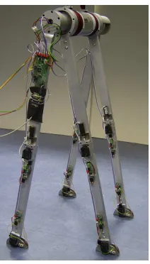
Simultaneously with my Master’s project, E. Dertien finished the design of the robot and con-structed it in his Master’s project. The robot walks quite stably. The robot is shown in figures 1.3 and 1.4, the design is described in detail in [4].
Figure 1.3:Dribbel, the first dynamic walker built at the University of Twente.
1.4
Goal of the project
Figure 1.4:Frame sequence of Dribbel walking. Reprinted with permission from Dertien [4].
these robots usually have a very small region of stability; only a minor disturbance is needed to cause a fall. Moreover, they have very wide feet, much wider than humans. This is not wrong in itself, but the question arises how humans can stabilize, even with narrow feet. Apparently there are more strategies than the ones already used in the prototypes.
One of these strategies is calledsideways footplacement(or lateral foot placement). This has already been investigated by some researchers (e.g. Kuo [7]), but new strategies for controlling the sideways foot placement might lead to more robustness against falling sideways. Creating and investigating such new strategies are the main topic of this research.
1.5
Report outline
In this report two different walker models are described that were used during the project. Chapter 2 describes a 3D bipedal walker with 8 degrees of freedom. The first few sections describe the simulation environment (section 2.1), the walker model itself (section 2.2), some modeling considerations (section 2.3) and a few submodels needed (section 2.4). The walker is first restricted to move only in two dimensions, and a controller is developed that keeps it upright in the forward/backward direction (section 2.5). As a sidestep on the research, a controller is implemented that controls the velocity of the walker by means of changing the ankle joint angles (section 2.5.2). After that the 2D motion restriction is removed and a controller is developed and investigated that should stabilize the walker in sideways direction by using sideways foot placement (section 2.6).
Chapter 3 describes a much simpler 3D walker model, consisting of a point mass as the hip and two massless, stiff legs. The dynamic equations for the walker are derived in section 3.2. Two controllers are developed to stabilize the walker in three dimensions, both using sideways foot placement. The first, described in section 3.4, uses pole placement on the linearized equations. The second, section 3.5, uses a property common to all limit cycles for control. Both controllers are compared in section 3.6.
Chapter 4 lists conclusions and recommendations. Some recommendations are just thoughts of the author and do not follow directly from the results described in this report.
Acknowledgement
Chapter 2
An 8-DOF 3D walker in 20-sim
As a part of this project, a model of a 3D walker with eight degrees of freedom was built in the simulation tool 20-sim. The model was produced with 20-sim’s new3D Mechanics Editor.
2.1
20-sim and the 3D Mechanics Editor
The application 20-sim [2], developed by Controllab Products B.V. is a very powerful simulation tool. One of its strengths is the fact that different modeling techniques, such as block diagrams, mathematical equations and bond graphs can be used together seamlessly. The energy based bond graph representation makes it perfect for describing multiple-domain systems. Many dif-ferent system analysis tools are provided, as are real-time 3D animations and interaction with Matlab.
One of the new features of 20-sim is the 3D Mechanics Editor. In this editor one can construct multibody systems in a very easy way. The rigid bodies can be interconnected by different types of translational and rotational joints. For each body the mass, center of mass and moment of inertia can be set. Also, for animation purposes, the shape, size and color of each body can be chosen.
The 3D Mechanics Editor produces an equation submodel that can be imported in 20-sim. Interaction of the different bodies with each other and with the environment is internally cal-culated by usingscrew theory[12]. Here, forces and torques are represented together in one 6-dimensional variable called awrench. Similarly, linear and rotational velocities are combined in a 6-dimensional variable called atwist. Note that this matches 20-sim’s energy based approach, as the product of a twist and a wrench is indeed an energy. Position and orientation of each body are kept in ahomogeneous matrix, which has the advantage of not having any singularities.
1-DOF Joints in the model are represented as 1-dimensional power ports. This makes it very easy to attach anything to such a joint; a constant force or torque for example can be applied on the joint by simply connecting aSe-element. The flow delivered by the element then represents the (linear or angular) joint velocity. The product of effort and flow is the injected power.
It is also possible to attach any number ofhinge pointsto any body in the 3D Mechanics Editor. This adds an extra 6-dimensional power port to the submodel, that can be used to apply external forces to the body (as a wrench) or, the dual of that, measure the velocity of that body (as a twist). Gravity acting on the system is handled internally by the submodel, so no external forces are needed for that.
The ease with which a complex multibody structure can be made and the flexibility of adding any number of power interaction ports to the model make the 3D Mechanics Editor very well suited for implementing a multi-degree-of-freedom walker.
Figure 2.1:Screenshot of the 20-sim-editor (left) and the 3D Mechanics Editor (right).
A screenshot of the 20-sim-editor and the 3D Mechanics Editor are shown in figure 2.1.
2.2
Model description
ϕankle=θ8
ϕknee=θ7
ϕsplay=θ6
ϕhip=θ5
ϕankle=θ4
ϕknee=θ3
ϕsplay=θ2
ϕhip=θ1
x y z
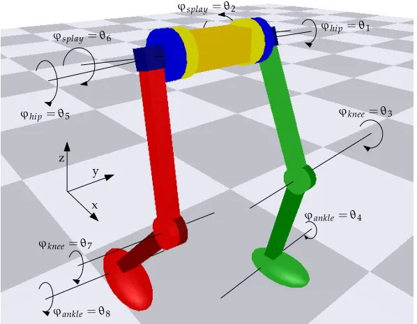
Figure 2.2:The 8-DOF 3D Walker.
Using the 3D Mechanics Editor, an 8-DOF two-legged walker was constructed. Figure 2.2 shows this construction, with all degrees of freedom indicated and named. Also the orientations of the axes of the reference frame Ψ0 are defined here. These are used throughout the whole report. The dimensions of the walker are inspired by the 2D walker that is currently under construction at the University of Twente and are shown in table 2.1.
2.2.1
Joints
2.2. MODEL DESCRIPTION
Size Mom. of inertia
Mass (m) (10−3kg m2)
Part (kg) l w h l w h
Torso 3.0 0.3 0.1 0.1 5.00 25.00 25.00
Hip 0.3 0.1 0.06 0.06 0.18 0.34 0.34
Upper leg 0.7 0.5 0.05 0.05 0.29 14.73 14.73
Lower leg 0.7 0.5 0.05 0.05 0.29 14.73 14.73
Foot 0.2 0.3 0.15 0.1 0.33 1.00 1.13
Table 2.1:The dimensions of the 8-DOF walker model.
rotates the foot up and down. Positive directions for the joints are the directions of the arrows shown in figure 2.2.
2.2.2
Upper body
Although it would improve stability to have an extending upper body (it brings the center of mass up) [13], it was chosen not to have one in the model. Instead, the torso was kept small and the mass was varied in some simulations to get a higher overall center of mass of the mechanism. This construction has the advantage over a real upper body that no active control is needed to keep the upper body upright.
2.2.3
Feet
The feet are modeled as ellipsoids that have approximately the size of a human foot. A big difference between human feet and these feet is the fact that these feet have only one contact point with the ground. This makes standing still harder, but ground contact simulations during walking easier.
Most dynamic walkers (both in simulation and in practice) also use curved feet instead of flat feet. Studies have shown that the behaviour of curved feet and that of flat feet with a compliant ankle (which is more or less what humans have) is quite similar: for both the center of pressure travels forward as the center of mass of the walker travels forward [9].
However, unlike many 3D walkers (such as Denise [13] and the unnamed walker of Collins, Wisse and Ruina [3]), the walker described here has ellipsoid feet instead of (nearly) cylindrical ones. Choosing cylindrical feet (with the cylindrical axes parallel to the world’s y-axis) would be obvious: a contact line segment provides friction in the rotational z-axis, which makes it easier to bring the swing leg forward with only a minimal reactive rotation around the z-axis. Wide feet also give more sideways stability, as they can provide a reactive torque if the walker tends to fall [9]. However, humans can walk on stilts, that neither have much rotational friction, nor guide the movement. Depending on the ground contact model, it is also easily possible to provide a large virtual friction coefficient of the foot for rotations around the z-axis, so the friction of cylindrical feet can be mimicked if needed.
2.2.4
Ports
2.3
Contact models
The model that comes from the 3D Mechanics Editor represents only a set of interconnected bodies; any interaction with the environment must be added later in 20-sim. This also holds for the interaction with the ground. If there were no interaction, the walker would just fall through it. Generally there are two ways to model contacts between two bodies (e.g. the foot of a walker and the ground): as a rigid contact and as a compliant contact.
2.3.1
The rigid contact model
The rigid contact model assumes the collision between the bodies to be instantaneous and (in this case) totally inelastic. The instantaneous nature is such that that the velocities of the bodies also change instantaneously. The mathematical equivalent is applying an impulse to the system; internally the new state after collision is calculated and the state variables are set to their new value directly.
After the collision has taken place, the two bodies make contact. During contact the relative velocities of the two bodies are restricted to less than 6 dimensions. For example, in the case of a point foot having contact with a frictionless ground, the foot can rotate freely and translate in the x and y-direction. But the movement in the (negative) z-direction is impossible. If the ground has an infinitely large friction, only rotations are allowed, no translations. Internally these restrictions are solved withlagrangian multipliers: a virtual force is constructed that, when applied, makes the accelerations in the ‘forbidden’ directions zero. The end result of this is that some states become totally dependent on the other states. Effectively they are then no real states anymore, because they cannot be chosen freely.
The mathematics involved in the rigid contact model (especially for a multibody system) are quite complex and extensive. However, the solution is known and described in detail in [6]. The authors also provided a tool that generates part of the 20-sim code needed to implement rigid contacts in a multibody model. Because the internal states of the system must be directly set, this method needs editing of the walker’s equation model. This is generally unwanted, because in doing so one destroys the modularity of the model.
Note that some advanced 20-sim programming techniques are required when implementing the rigid contact model. Therefore it is strongly advised to read appendix A, that discusses these techniques.
2.3.2
The compliant contact model
The compliant contact model is mathematically much simpler. At the moment the two bodies make contact, a (possibly non-linear) spring and damper are attached between the two contact points. The spring and damper decelerate the bodies in such a way that a collision is simulated. As the deceleration is not instantaneous, the bodies do penetrate each other a little bit. If the system is critically damped or overdamped, the collision is totally inelastic.
If a linear spring and damper were used, the compliant model would suffer from disconti-nuities in accelerations and the so-calledsticky effect. This can be solved by using the nonlinear
Hunt-Crossley modelas described in [5]. This model calculates the normal forceFNbetween the two bodies as:
FN(t) =
k xn(t) +λxn(t)x˙(t) x≥0
0 x<0
wherexis the penetration depth,kandλthe spring and damper parameters andna real number, dependent on the shape and material of the object.nis usually close to unity.
2.3. CONTACT MODELS
friction behaviour, including static, coulomb and viscous friction. Different models can be found in the literature that approach this type of friction. A relatively simple one, also used in the 20-sim block SCVS-friction, is the following model:
FF =FN·
µc+ (µst−µc)e−
˙ x vst
2!
sgn(x˙) +µvx˙ !
where FF is the resulting friction force, FN is the normal force as calculated above, andµc,µst, µv andvst are the model parameters. In order to avoid discontinuities around ˙x = 0, the sgn
function can be replaced by a tanh function with a very steep slope:
sgn(x˙)≈tanh(x˙/vsl)
wherevslis small (e.g. 0.001). As 20-sim provides integration methods with adaptive step sizes,
it can cope perfectly with such steep slopes.
2.3.3
Comparison
Both the rigid contact model and the compliant contact model have their advantages and disad-vantages.
The rigid contact model does not use stiff springs, so the simulation step length can be larger without making a too large error. However, the mathematics are more complex, so a simulation step takes more time to be calculated. No actual experiments were done, but it is estimated that the rigid contact model outperforms the compliant model with respect to simulation speed.
Another advantage of the rigid contact model is that the two contacting bodies are exactly touching each other instead of penetrating each other (a few mm if the springs are chosen not too stiff). This could make a huge difference in walking, because the clearance between the ground and the swing foot is also only a few mm. If the penetration depth of the stance foot happens to be just larger than the ground clearance of the swing foot, the swing foot will hit the floor, which would not have happened if a different floor model was chosen.
On the contrary, the compliant contact model wins on ease of implementation and flexibility. The latter is very important. In the rigid contact model the contact point is internally seen as a non-movable joint that imposes restrictions to the state. These restrictions prevent sliding of the contact point, so slipping contacts cannot be modeled. But some movies of already produced experimental 3D walkers (e.g. [13]) show that the feet of the walker occasionally do slip. The rigid contact model can not handle this, the compliant contact model can.
In principle a combination of the two can be made. The normal forceFN could be calculated by
the rigid contact model, thereby solving the penetration depth problem. The compliant friction model could then be used to calculate the friction forces, allowing slipping. However, imple-menting this would again destroy modularity (as part of the contact forces are computed as being internal forces although they actually result from external interaction).
Moreover, the compliant forces only work during contact, not at the instant of collision. The rigid contact model however, does use that instant to apply an impulse that approximates the real world’s very short (but not infinitely short) moment of deceleration. During that short mo-ment friction works too, so that should be implemo-mented in a similar way: a frictional impulse. Unfortunately it is not possible to simply use the (linear) rigid contact equations for solving the (non-linear) friction problem. So, a new set of equations should be found to make the combined model work.
2.4
Submodels
Apart from the model of the walker itself, other submodels are needed as well, such as controller blocks, joint actuators and contact modeling blocks. A number of these blocks were implemented as separate 20-sim submodels so that they could be used in a flexible way. Some of these sub-models are described in more detail in this section.
2.4.1
Kneelock, kneefix, knee-end
These blocks were all primarily designed to operate on the knee joints of the walker, but they can be used on any joint. They all limit the motion of the joint in certain circumstances.
The kneelock works much in the same way as a door: if the knee is unlocked (door lever pulled down), the lower leg (door) can swing freely. If it is locked (door lever released), the leg (door) can still swing freely, except for one point (leg stretched or door closed) where it is held in that position until the next unlock. It can be used to keep the leg straight (knee locked) if the leg is stance leg, and bendable (knee unlocked) if the leg is swing leg. The kneelock needs information about the absolute position of the knee. This is information that is not given through the power port. Therefore, it makes use of the global variabletheta, which holds all joint angles.
The knee-fix is much simpler: it just holds the lower leg in its starting position (relatively to the upper leg, not to the world). Two versions of this block were made; one with a stiff PD-controller that holds the leg in place, and one with the 20-sim-functionconstraint. The latter is better; it iteratively finds a force that makes the joint’s angular acceleration exactly zero. However, it can only be used with the MBDF integration method and it cannot be in a conditional statement. So, the PD-controller is much more flexible. The knee-fix blocks only need a power port to connect the joint, so they are very easily connectible.
The knee-end block delimits the movement of the (knee) joint to a certain range. At the bound-aries of the range a PD-controller prevents further movement, much in the same way as the compliant contact model described in section 2.3.2.
2.4.2
Floor
As already stated in section 2.3.3, the compliant contact model was used for ground modeling. For handling contacts between the (ellipsoid) foot and the ground, a submodel was made that features:
• realistic friction in translation and in rotation around the z-axis, including stiction and vis-cous and coulomb friction, based on the equations of section 2.3.2,
• rolling (frictionless),
• Hunt-Crossley equations for the z-component,
• Intelligent on/off mechanism that can be used to solve foot scuffing by temporarily ignor-ing the ground.
The submodel needs two connections to the walker model: the absolute position and orien-tation of the foot as an homogeneous-matrix (denoted byHs0) and the 6-dimensional power port
associated with a hinge point in the center of the foot (Tss,0/Ws). Also the foot size is needed as a
set of parameters.
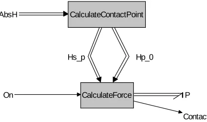
The floor model consists of two submodels, as shown in figure 2.3. The complete source code of both subblocks can be found in appendix B.
Thecalculate-contactpointblock determines which point of the ellipsoid has the lowest z-coordinate; it is this point that will make or have contact with the floor (atz=0). It puts a frame
2.4. SUBMODELS Hs_p Hp_0 AbsH P Contact On CalculateContactPoint CalculateForce
Figure 2.3:The 20-sim block model of the compliant floor.
of this frame expressed in world coordinates (H0p) and the position of the foot Ψs expressed in
contact point coordinates (Hsp).
Thecalculate-forceblock determines the wrench resulting from the contact. For the block the position of the contact point is known; if its z-coordinate is smaller than or equal to zero, there is ground contact. If so, a wrench will be exerted on the foot. This wrench depends on the position of the foot (especially the penetration depth) and on the velocity of the foot (in particular the velocity of the contact point). Therefore, it is convenient to express the velocity of the foot,
Ts•,0, in the contact point frameΨp:
Tsp,0=
ω v
=AdHp s T
s,0 s
By doing this, we separate rotation (rolling) from translation (slipping). Nowωindicates a pure rotation around p, v indicates a pure translation (so a non-zerov means the object is slipping).
The normal force FN can now be calculated with the Hunt-Crossley equation and the use of
pzand ˙pz. ThisFNis in the direction of the z-axis ofΨp.
Now let us call the euclidean projection ofwon the xy-plane vxy (so, this is simplyv with its z-component ignored). As the translational friction is non-linearly dependent on|vxy|, we cannot simply treat the x and y direction separately and then add the results; this only works in linear cases. Instead, we have to calculate the friction based on the total velocity and only then decompose it in x and y direction:
FF,xy
=F vxy FF,x=
vx vxy FF,xy
; FF,y= vy vxy FF,xy
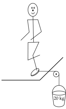
where F is the friction equation as described in 2.3.2, depending linearly onFN and nonlinearly on|v|. The friction parameters were estimated by doing simple imaginary tests such as: ‘Could an 80 kg person stand on one foot if a sideways force of 200 N is pulling the foot? — I guess so, so the friction coefficient (including stiction) must be larger than 200800 =0.25.’ (See figure 2.4).
As for rotations only rotation around the z-axis of the frame Ψp has friction. For this the
friction function is used withωz as parameter: FF,ωz =F(ωz). We now have all forces to build
up the resulting wrench (expressed inΨp):
Wp=
0 0 FF,ωz FF,x FF,y FN
20 kg
Figure 2.4:Illustration of an imaginary test done in order to estimate friction parameters.
Ws =AdTHsp
Wp
The floor can be turned on and off for each foot separately. If the floor is turned off, the simulation acts as if there were no floor at all; the foot can penetrate it freely, without experiencing a force. This is a useful feature if one wants to do some experiments without too much concern about foot scuffing.
If the floor is turned back on, it is first checked if the foot is above the ground. If not, the floor is not activated until the foot is high enough. This way, the floor can already be turned on while the foot is still scuffing, which simplifies the timing.
Using the floor submodel in 20-sim is easy. Just make sure there is a hinge point in the ellip-soid object, connect theAbsHand power port, set up the size of the ellipsoid in the calculate-contactpointblock and simulate.
2.4.3
Aligner
It is quite hard to make a 3D walker walk when starting from scratch. Everything has to be right, if one thing is not, the walker will fall. Therefore it is convenient to split up the work into smaller steps so that not all problems have to be solved at once. Thealignerblock makes it possible to let a 3D walker walk as if it were a 2D walker, and then gradually add more of the third dimension to it.
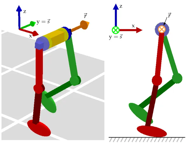
The aligner submodel is a block that applies an external wrench to the body associated with the hinge point it is attached to. The wrench is such that it aligns a certain vector~r, fixed in the body frame, to a certain vector~sfixed in the world frame. If the body is the walker’s torso, ~ris chosen to be the torso’s local y-axis and~sis chosen to be the world’s y-axis, the walker is prevented to rotate around its x-axis (which would cause sideways falling) and its z-azis (which would cause a change of walking direction). Indeed, these restrictions make that only movements are possible that a 2D-walker can do: the 3D problem is reduced to a 2D problem (see figure 2.5). The wrench is internally determined by a PD-controller. By adjusting the Kp andKd of the
controller, one can choose any degree of ‘helping’ by the aligner. Very high values restrict the walker’s movement strictly to 2D, lower values give a limited 3D behaviour. Zeros disable the aligner, leaving the full 3D system as it is. This is very useful for designing controllers; one can gradually increase the demands for them in this way.
con-2.4. SUBMODELS
z
~
r
y=~s
x
z
x
y=~s
~
r
Figure 2.5:A perspective (left) and a side (right) view of the 3D walker, showing that if the torso’s ~r-axis is aligned with the world’s~s-axis, the walker indeed looks like (and behaves like) a 2D walker. This figure also makes clear that it is allowed for the body (torso) to rotate around the ~r-axis without destroying the 2D behaviour.
troller needs an orientation error~eand a rotational velocity error ˙~e. The~eshould represent how misaligned both vectors are. The vector product is a good measure for this:
~eb =~rb∧~sb =~rb∧
Hb0−1~s0
⇒
|~eb|=|~rb| · |~s0|sinα=sinα≈α
where~•0 represents the vector~• expressed in world coordinates,~•b represents the vector~•
expressed in body coordinates, and it is assumed that~rand~sare unit vectors and that the angle
α between the vectors is small. The direction of~eis the axis along which the body should be rotated to realign~rwith~s.
As the orientation of the~r-axis does not change when the body rotates around that~r-axis, the body may have any rotational velocity around~r. Rotating around the~r-axis is not an error, so the ~r-component of the body’s rotational velocityω~ should be excluded from the rotational velocity error ˙~e. This can be done by taking the projection ofω~ (thisω~ is the first 3 elements of the twist
Tbb,0) on the plane perpendicular to~r:
˙
~eb=~rb∧ω~ b∧~rb
with the same assumptions as above. The PD-controller is now simply:
Wb =
Kp·~eb−Kd·~e˙b T
0 0 0
whereKpand Kdare positive controller parameters. The wrench is already expressed in body
Walker
1 1
FixPD3
FixPD3
FixPD4
FixPD4
Aligner PDcontrol
rAnkleControl
f
KneeLock1
KneeLock1
KneeLock2
KneeLock2
endstop1
endstop2
WalkingState
FootAngleControl
lAnklePD
Cam_movement
Cam_movement
FloorLeftFoot Controller
FloorRightFoot
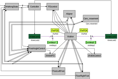
Figure 2.6: Block diagram of the 3D walker with all control blocks attached for 2D simulation. The aligner block (top center) holds the walker in a 2D plane.
2.5
Simulation in 2D
With the help of the aligner block the movement of the walker model was restricted to two dimen-sions. Also the splay joint angles were fixed by using knee-fix blocks. The work of Beekman [1] was used as a starting point for the simulations in 2D.
The graphical 20-sim model is plotted in figure 2.6. The hip joints and ankle joints are actu-ated, they all have a PD-controller attached. The knee joints are equipped with end stops and a knee-lock, apart from that the joint movement is unactuated.
Thewalkerstateblock determines in which phase of the step the walker is. A full cycle consists of four states, being:
• State 1: right leg is stance leg, left foot is still behind right foot, • State 2: right leg is stance leg, left foot has passed right foot, • State 3: left leg is stance leg, right foot is still behind left foot, • State 4: left leg is stance leg, right foot has passed left foot.
These four states are used in the controller block to set the hip setpoints, operate the knee locks and to determine the behaviour of the ankle joints. If needed, the controller can also turn off and on the floor for each foot to artificially avoid foot scuffing. A functional overview of the controller block is given in table 2.2.
2.5.1
Simulation results
2.5. SIMULATION IN 2D
Left leg Right leg
Stance hip knee- ankle floor hip knee- ankle floor
State leg [rad] lock [rad] (opt.) [rad] lock [rad] (opt.)
1 right -0.3 unlocked -0.25 off +0.3 locked 0∗ on
2 right -0.3 locked -0.25 on +0.3 locked 0 on
3 left +0.3 locked 0∗ on -0.3 unlocked -0.25 off
4 left +0.3 locked 0 on -0.3 locked -0.25 on
Table 2.2: Functional overview of the controller of the 8-dof walker in the 2D simulation. The numbers are all setpoints for the different PD controllers. Note that ‘locked’ means that the lower leg can still rotate freely, until it reaches its extended position; only then the leg will be kept in position. The two setpoints marked with an∗ indicate that these setpoints are controlled when using ankle actuation as described in section 2.5.2.
• The aligner block is not infinitely stiff, therefore the hip of the swing leg drops a few mm relatively to the hip of the stance leg. Consequently the foot of the swing leg is also a few mm lower than it should be. A solution is to increase the aligner stiffness, which leads to larger simulation times. Also a different aligner block could be made that makes use of 20-sim’sconstraintfunction (see section 2.4.1), but that has the disadvantage that it can only be turned on or off, nothing in between. A last option would be to decrease the torso width, but that involves changing the walker model, which is also unwanted. It was chosen to increase the stiffness of the aligner toKp= 1500,Kd =100, which results in a hip drop of about 2 mm.
• The compliant floor model lets the stance foot penetrate the floor a little. The result is that the total walker, including the swing foot, is closer to the ground. WithKp = 10000,
Kd=30000 the penetration depth, and thus the loss in ground clearance for the swing foot
is about 8 mm.
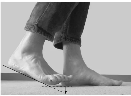
• The feet are so big that the toes hit the ground easily. The bending of the swing leg makes the foot rotate so that the front of the foot goes through the ground. Humans solve this problem by pointing their toes up (figure 2.7). The simulated walker has no toe joints, so it has to lift its whole foot up to avoid hitting the ground.
Property Value Remarks
Step time 0.68 s
Step length 0.45 m
Forward velocity 0.66 m/s
Ground clearance 2 mm
Power consumption 2.3 W
Peak power consumption 140 W Once each step, for about 0.02 s
Specific resistance 0.07 – P/(m g v)
Table 2.3:Properties of the walker’s gait when walking in 2D
After manual parameter ‘optimization’ the ground clearance of the foot during normal gait was 2 mm. If a stiffer floor model would be used, in which the stance foot does not lie 8 mm under the floor, the ground clearance would be almost 1 cm, which is good enough.
The PD controller in the hip has parametersKp=300,Kd=100 that were chosen after some
trial-and-error simulations. The actuator consumes 2.3 W, which results in a specific resistance (also calledspecific cost of transport; the amount of energy required to carry a unit weight a unit distance) of 0.07, which is quite good (humans do 0.38 [11]). The maximum power dissipated is 140 W (only for 0.02 s), which is really a lot. The problem is the choice of the PD controller with a fixed setpoint instead of a smooth path. A different controller could do this much better. The reason that a PD controller with fixed setpoint was chosen anyway is because it is simple and effective [13, 1].
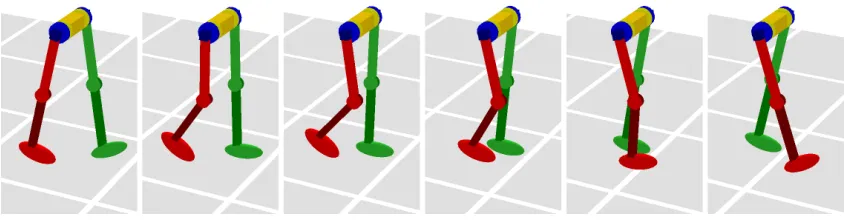
Figure 2.8:The 3D walker walking in 2D.
In the resulting simulation the 2D walker walks stably, with a naturally looking gait. The ground clearance is quite large, which is good. In figure 2.8 a series of pictures is shown of the walking system. Some properties of the gait are listed in table 2.3.
2.5.2
Velocity control by means of ankle actuation
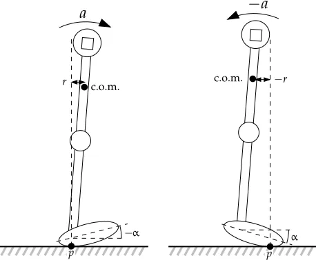
A new control feature was implemented in the ankles, which makes it possible to control the forward velocity of the hip. The principle used here is that by rotating the stance foot, the contact point can be shifted forward or backward, which affects the forward/backward acceleration due to gravity (see figure 2.9). A very simple controller was implemented that tries to give the torso a constant forward velocityvre f by adjusting the ankle setpointα according to the following
equation:
α=K·vtorso−vre f
2.6. SIMULATION IN 3D
c.o.m.
r
−α
a
c.o.m.
−r
α
−a
p p
Figure 2.9: Velocity (or actually: acceleration) control by ankle rotationα: the position of the contact pointpinfluences the accelerationadue to gravity working on the center of mass (c.o.m.). Left: the contact point behind gives a forward acceleration. Right: the contact point in front gives a backward acceleration.
A simulation run was done in which thevre f was slowly increased from 0.1 m/s to 0.65 m/s.
Indeed, the walker increased its speed accordingly; the step timetstepvaried from 1.24 s during the first steps to 0.64 s during the last steps. See figure 2.10. It should be noted that the controller was only active during state 1 and 3. It is during state 2 and 4 that the walker gains kinetic energy from falling forward; as this part of the step is uncontrolled on the ankles, it is no wonder that the forward velocityvtorsoincreases to much more thanvre f.
As the main focus of the project is on sideways stabilization, optimization of this controller was left behind. It is expected that good results can be obtained by having a time-dependent
vre f(t)that matches the velocity path of the desired gait.
2.6
Simulation in 3D
The three-dimensional walker now walks in 2D, with the help of the aligner block. The next step is gradually removing the influence of the aligner and develop algorithms that keep the walker upright in three dimensions. Because the walker with eight degrees of freedom is quite complex (too complex to describe its motion with simple mathematical equations), it was decided to make the walker behave a little simpler. This was done by pointing the feet straight up, so that it walks on its heels. Because the heels are small, the feet now behave almost like point feet instead of (rolling) normal feet.
Also, the default splay angel for both legs was set to −0.2 rad, which puts the feet almost under the center of mass (see figure 2.11) instead of precisely under the hips. This might look a bit strange, but humans do this too: the sideways distance between the feet of a normally walking person is only a few cm. As the feet of the walker are almost under its center of mass, the sideways excursions of the torso are not so large, so only a small force is needed to control it. The aligner stiffness was reduced toKp=100,Kd=13.
Figure 2.10:Simulation results of the 2D walker accelerating. The bottom graph shows the angle of the left ankle. It can clearly be seen that the behaviour changes when the desired velocity changes.
The controller performed not well at all, so it was adapted by including the sideways velocity of the torso. Unfortunately, manual tuning has so far not resulted in a series of parameters that stabilize the gait.
After trying to use the rotational velocity of the torso around the stance foot’s contact point and different methods to keep the torso straight, it was decided that something better was needed. With the aligner block still at Kp = 100, a simple trajectory predictor was built that, at any time within the current step, predicts the y-position of the torso at the expected end time of the step. It then calculates aϕsplayfor the next step such that the trajectory of the next step ends up in a desired y-position for the hip (see figure 2.12). After careful manual tuning of the parameters of the two controllers, the walker could do 10 steps before stumbling and falling forward (when the splay controller was switched off, it did only 2 steps and fell sideways, even with the aligner on). However, the gait was not very smooth and the feet slipped quite often.
Many simulations were done in the search for good parameter values, but they did not result in a series of parameters that made the system walk stably forever. As each simulation took at least 30 seconds, this was not very fast way of finding stable walking behaviour. Moreover, the main interest is not in finding a set of tweaked parameters for some controller with which the system happens to walk, but in finding and understanding a control method that just works (with a whole range of possible parameters) because it is a good method. Unfortunately, the 8-dof walker is just too complex to build and understand such a controller from scratch.
2.6. SIMULATION IN 3D
x y z
Figure 2.11:The 8-dof 3D walker as it is being used for 3D simulations. The legs are bent a little inwards, to get the feet more or less under the center of mass. The walker walks on its heels, which behave more or less like a point contact.
current step next step
2. predicted position at the end of the step
3. desired position at the end of next step 1. current
hip position
4. calculated foot placement for the next step
walking direction
Chapter 3
A very simple 3D walker
In order to explore the 3D behaviour of a walker in a more mathematical way, a very simple system was designed and simulated in 20-sim and Matlab. The equations of the system were (partly) derived with the help of Maple.
3.1
The walker
The walker that is used in this chapter has the following properties:
• The hip is modeled as a point of massm, • The legs are attached to the hip in this point,
• The legs are massless, have no knees and have length`,
• The feet are modeled as point feet and have no mass. A consequence of the massless legs and feet is that one cannot move the legs and feet by applying a force, as the acceleration would be infinite. Therefore, instead of using a force as an input, the position of the legs is used as an input directly,
• Each leg has two degrees of freedom: forward/backward position (ϕhip) and sideways
position (ϕsplay).
• Active control of the system is only done by choosing an appropriate position for the swing leg. This type of control is calledfoot placement.
Figure 3.1 (left) shows how the joints of the walker work. Note that this figure is only a schematic drawing of the kinematics, the joints are assumed infinitely small and all exactly at the same point in the hip. This is shown in figure 3.1 (right).
Although the 3D walker can walk in any direction (and it does that too, if a disturbance is applied), we assume that the walker’s heading is always in the direction of the positive x-axis. This is done for angular reference purposes. If the splay angleϕsplay is constant, the foot is moving in the xz-plane only (fore-aft motion); the y-coordinate of the foot remains constant.
The walker has a stance leg and a swing leg, denoted by the subscripts: stand sw. These subscripts are only used if there is a chance of confusion. During the simulation of the step, the stance leg angles (ϕhip,st,ϕsplay,st) are calculated by the integration method, by using the formulas given in section 3.2. The swing leg angles (ϕhip,sw,ϕsplay,sw) are direct inputs (and the only inputs) of the system (and therefore they are no states of the system). Because the legs are massless, they do not influence the dynamics of the system (apart from contact constraints of course).
stance leg
swing leg
ϕ
hip,stϕ
hip,swϕ
splay,stϕ
splay,swx
y
z
stance leg
swing leg
ϕ
hip,stϕ
hip,swϕ
splay,stϕ
splay,swx
y
z
Figure 3.1:The ‘very simple walker’. In order to make clear how exactly the joints work, a draw-ing (left) is provided where the joints are drawn separated. However, the real model has all joints in the same point (right). Positive rotation angles for the joints are indicated with arrows in the right figure.
of the old swing leg can be used as initial angles of the new stance leg. The new swing leg instantaneously gets a position defined by the input values, so it is actually not swinging. As a consequence no foot scuffing can occur.
For both the stance leg and the swing legϕhipis positive if the leg is stretched backwards (so that the foot is behind the hip, or,xf oot <xhip). If the leg is stretched forwards, the angleϕhipis
negative. So, for a normal walking gait, where the stance leg travels from the front to the back (relatively to the hip),ϕhip,st starts negative and becomes positive as the hip passes its highest
point. This gives a ˙ϕhip that is positive. For a normal gait theϕhip,sw will be negative at foot
impact, whereasϕhip,stis positive.
For both legs,ϕsplayis positive if the leg is pointing ‘outwards’, as seen from the front. For
the left leg, it means that the foot is left of the hip (yf oot > yhip), for the right leg it means that
the foot is right of the hip. Inside the model there is no real awareness of left and right (only for viewing purposes), the only important thing for the model is that the stance leg’s positive direction is opposite to the swing leg’s positive direction.
We denote the state of the system at any time by
x=
ϕhip
˙
ϕhip ϕsplay
˙
ϕsplay
where all theseϕ’s refer to the stance leg. The swing leg variables are inputs rather than states, they are denoted by
u=
ϕhip ϕsplay
where bothϕ’s refer to the swing leg. The states at the beginning of stepkare denoted byxk. The
3.2. MATHEMATICAL DERIVATION OF THE MODEL
step ends and influence the starting conditions of the new step). The inputs at the end of stepk
are denoted byuk.
If there were no noise and the state at the beginning of step kwere known (beingxk), any
state in the future can be calculated simply by integration (section 3.2.1) and applying the impact equations (section 3.2.2). Using this, the statexk+1at the beginning of stepk+1 can be found,
which is dependent only on the former state xk and the input uk. Mathematically this can be
described with the (non-linear)stride functionS:
xk+1=S(xk,uk)
Note that not all states and inputs will deliver a new state for the next step. As an example, consider a state and input that describe a system that is standing still. This situation will never reach a new step, so there will be noxk+1. Assume that anx∗ andu∗ can be found for which
holds:
xk+1=S(xk,uk) wherexk+1=xk=x∗anduk=u∗
By induction it can be proven thatxk+n = x∗ for eachn ≥ 0 (assuming that the input is kept at u∗). If at a certain point the statex∗ is reached, the system will subsequently do an infinite number of identical steps and it will never fall. In other words: the system walks. The periodic cycle that contains the statex∗and inputu∗is called alimit cycle.
3.2
Mathematical derivation of the model
3.2.1
Equations of motion
The direction choice ofϕsplay,standϕsplay,swhas been such that it has no relation at all to left and
right. Consequently, the resulting dynamic equations will neither have any relation to left and right. We only bring a choice for left and right for viewing purposes, not for calculating purposes. However, while deriving the dynamic equations, some use has been made of the cartesian frame. For the mapping from the anglesϕto the cartesian coordinates(x,y,z) we do need to choose which leg is the left leg and which is the right. So for the derivation of the equations we assume that the left leg is the stance leg and the right leg is the swing leg. As expected, the final dynamic equations are independent of y(the left-right axis) again, so indeed they have no relationship to left and right any more.
If the position of the stance foot is taken as the origin, the position of the hip (~phip) can be expressed as follows, at each timet:
~phip=
xhip yhip zhip
=
`cosϕsplaysinϕhip
−`sinϕsplay
`cosϕsplaycosϕhip
where~p,x,y,zand allϕ’s are dependent ont. It is obvious that here allϕ’s are related to the stance leg (ϕ•,st), as the position is calculated relatively to the stance foot. The motion of the
hip during one step can be calculated with the Euler-Lagrange equations. The lagrangian is the kinetic co-energy minus the potential energy:
L=T−V
=
1 2ml
2ϕ˙2
splay+ϕ˙2hipcos2ϕsplay
−m g`cosϕhipcosϕsplay
of the stance leg due to the moving hip mass:
¨
ϕhip =
gsin(ϕhip) +2`ϕ˙hipsin(ϕsplay)ϕ˙splay
`cos(ϕsplay)
¨
ϕsplay = −
sin(ϕsplay)`ϕ˙2hipcos(ϕsplay)−gcos(ϕhip) `
wheregis the gravitational acceleration.
These equations (being the motion equations of an inverted spherical pendulum, expressed in
ϕhipandϕsplay) can be used by an integration method to calculate the statexat each timet. The
path calculated is the path that the hip follows during one step. As already stated in section 3.1, the swing leg does not influence the system, as it does not make contact with the floor during this phase of the gait. Therefore it is no wonder thatudoes not appear in the equations.
At the end of the step foot impact occurs, for which some more equations are needed.
3.2.2
Impact equations
At the end of a step, when the swing foot hits the ground, we speak of foot impact. On impact the old swing leg becomes the new stance leg, and the new swing leg’s position is set directly according to the inputs. In this model the contact and support transfer is assumed to be totally inelastic and instantaneous, so some energy is lost. This can be modeled with an instantaneous change of the momentum of the system. The state of the system just after impact (as a function of the state just before impact) can be calculated by using the impact equations described in this subsection. The impact equations combine two purposes:
• Calculate the kinetic energy loss due to the impact of the foot,
• Express the angles and angular velocities of the hip in terms of the angles of the new stance leg.
The notational convention used here for describing the impact equations here is as follows:
• Pre-impact variables are superscripted−, e.g.ϕ−hip,• meaning: the hip-angle, an infinites-imal small time before impact. Similarly, post-impact variables are superscripted+. The values of the input u are only important just before impact (they act as an input for the impact equations), not after it. So, no confusion can be made, and the−is omitted.
• Leg naming is simply according to the function of the leg before and after impact: ϕ−•,st
refers to the pre-impact stance leg,ϕ−•,swandϕ+•,st refer to the leg that is pre-impact swing leg and becomes stance leg after impact, andϕ+•,swrefers to the new (post-impact) swing leg.
• Only the stance legs (the old stance leg just before impact and the new one just after impact) are important for the impact equations. The swing leg is not used in the equations, so all variables refer to the stance leg. Because there is no risk of confusion, the subscriptstwill be omitted.
3.2. MATHEMATICAL DERIVATION OF THE MODEL
˙
ϕ
−˙
`
+˙
ϕ
+Figure 3.2: Sketch of a 2D walker at the moment of impact. The hip instantaneously changes direction and speed; from ˙ϕ−to ˙ϕ+.
the impulse were too large, the hip would get a positive velocity in the direction of +` which would make the foot leave the ground again, making the collision elastic instead of inelastic). So, directly after impact, the impulse will set the component −`˙+ to zero. The kinetic energy that is dissipated by this impulse is lost. After foot impact the velocity of the hip is just ˙ϕ+. Mathematically the decomposition can be seen as a simple mapping from one polar coordinate frame (Ψ− = (ϕ−,`−)) to another (Ψ+ = (ϕ+,`+)). Because the legs have a fixed length`, the ˙
`−is always zero.
In three dimensions the only thing that changes is that we have two ˙ϕvariables to cope with: ˙
ϕhipand ˙ϕsplay. An easy way of doing the mapping is by using cartesian coordinates as an
inter-mediate step. The two mapping functionsMare dependent on the actual spherical coordinates of the hip:
˙
ϕ−hip ϕ−splay
`− M ϕ− hip ϕ− splay `− =⇒ ˙ x y z
M−1 ϕ+ hip ϕ+ splay `+ =⇒ ˙
ϕ+hip ϕ+splay
`+
Although ` is constant and therefore could be omitted as a variable in the formula above, it is preferable to leave it in, for a couple of reasons. Firstly, it makes the equations bijective and thus invertible. This way, we preserve time-symmetry, which is needed later on. Secondly, having ˙`+ makes it easy to calculate the impact energy loss: this is simplyEloss = 12m(`˙
+
)2. A
last advantage of having`in the formula is that one can use it to inject energy into the system by using a nonzero value for ˙`− at the exact moment of impact. This is described in detail in section 3.2.3. Note that the nonzero values for ˙`−and ˙`+ occur only for an infinitesimally small period of time, so the legs don’t become shorter or longer because of this.
By using Maple, formulas were derived to calculate(ϕ˙+hip, ˙ϕ+splay, ˙`+). The two other states,
ϕ+hipandϕ+splayare the angles of the new stance leg, which was the swing leg before impact. The position of the swing leg was simply equal to the inputu. During impact the angles of the leg do not change, hence the anglesϕ+hipandϕ+splayare simply equal tou.
All impact equations can be combined in the (non-linear) function IE:
x+=IE x−,u
ϕ+hip
˙
ϕ+hip ϕ+splay
˙
ϕ+splay = u1 ˙
ϕ+hip(x−,u)
u2
˙
ϕ+splay(x−,u)
3.2.3
Energy injection
At each step the system loses a certain amount of energyElossdue to foot impact. In order to walk forever, we need to add energy each step to compensate for this. One way of adding this energy is by applying a force (or more correct: an impulse) along to the old stance leg, at the instant of foot impact. The impulse can be interpreted as resulting from the old stance leg being extended (simulating the push-off of the human ankle during normal gait). The kinetic energy added to the system will be denoted byEadd. In order to keep the energy level of the system constant, as
much energy should be added as is lost during a step, thus:Eadd =Eloss.
In the previous section the variable ˙`−was already introduced, and it was also indicated that this variable could be used for energy injection. The amount of energy added to the system is, analogous to the energy loss described earlier:Eadd= 12m(`˙
−
)2.
The signs of ˙`−and ˙`+are easily determined by examining the configuration: the pre-impact stance leg should be extended in order to give the walker some forward energy, so ˙`− is posi-tive. If the new stance leg hits the floor, it will experience a compressing force (instantaneously counterreacted by the leg itself), so ˙`+is negative. This gives the following equations:
Eadd=Eloss⇔ 1 2m(`˙
−
)2= 1 2m(`˙
+
)2⇔`˙−=−`˙+
The impact equations (described in the previous section and shown in appendix C) reveal that ˙`+depends on ˙`−(so alsoElossdepends onEadd), so the above equation gets a little bit more complex. Fortunately, the dependency happens to be not so difficult and can be written as:
˙
`+ =a`˙−+b
whereaandbare only dependent on the (fixed) leg length`, the state just before impactx−and the inputu, and are thus known. Substitution of ˙`+and rearranging gives us the desired ˙`−. As an indication for the what the resulting equations look like, aandbhave been substituted too, giving the totally expanded equation:
˙
`−= −b 1+a
=`cosu2cosu1sinϕ−hip cosϕsplay− ϕ˙−hip+cosϕhip− sinϕ−splayϕ˙−splay
+sinu1sinϕ−hip sinϕ−splayϕ˙−splay−cosϕ−hipϕ−splayϕ˙−hip +` cosϕ−splayϕ˙−splay sinu2.
1+cosu2 cosϕ−splay
sinϕ−hip sinu1+cosϕ−hip cosu1
−sinϕ−splay sinu2
This type of energy addition was always used during this research. In fact, it was imple-mented as a part of the impact equations. The resulting impact equations (thus including energy addition) can be found in appendix C. It is these equations that were used for simulation and mathematical analysis (see also figure 3.3).
3.3
Implementation and simulation of the model
3.3. IMPLEMENTATION AND SIMULATION OF THE MODEL
Impact equations
including
Energy injection Equations
of motion
RR
xk x− xk+1
k x
+
k+1
u
uk
impact detection
Walker
Stride function S(xk,uk)
Figure 3.3: A block diagram of the mathematical structure of the walker. The stride function S, used throughout the rest of the chapter, includes the equations of motion and the impact equa-tions, including the energy injection mechanism.
3.3.1
The complete model in 20-sim
Having the equations of motion and impact equations (including energy addition), all ingredients are present to build a simulation block of the walker. In order to be able to do different simulation tests, a block for 20-sim was built as well as a set of Matlab files. Exporting the long formulas was really simple with the use of Maple’s newMatlabcommand, that directly converts the used formulas to ready-to-run Matlab code. The code obtained is also fully 20-sim-compatible.
The 20-sim model is discussed in more detail here; the code itself can be found in appendix D. For (some of) the Matlab code see appendix E.
Figure 3.4 shows the appearance (left) and a schematic representation of the inner structure of the 20-sim model (right). Although it is perfectly possible in 20-sim to actually build the model in such a graphical representation, it was decided not to do this and keep everything together in one equation submodel. However, the blocks are still clearly recognizable in the code.
The blocks inside the dashed rectangle describe the walker itself. The three blocks outside it are auxiliary blocks for visualization and controller-connection purposes.
The dynamic equations block simply calculates the accelerations ¨ϕhip and ¨ϕsplay from the state
x, using the equations from section 3.2.1. These accelerations are directly fed into the resettable integrator block that updates the statex.
The impact equations block continuously calculates a new statex+from the current state. The output of this block at each time can be seen as the new statex+if impact would have occurred at that time.
The foot impact detection block fires an ‘impact event’ when it detects the swing foot hitting the ground. It does this by calculating the cartesian coordinates of the hip and the swing foot relatively to the stance foot, and keeping an eye on thez-coordinate of the swing foot. If it has a negative derivative and it crosses zero, it is seen as a foot impact.
As soon as the resettable integrator receives the fired impact event, it sets its output statex
equal to its ‘new-value’-input, so the state becomesx+, just as intended.
An extra advantage of the way the foot impact detection block is split is that the hip and foot positions can also be used as an input for the simulator’s animation view. Some extra animation-related variables are set in the
![Figure 1.1: The principle of making a 2D walker with a guiding system [10].](https://thumb-us.123doks.com/thumbv2/123dok_us/1167990.1146927/10.595.177.425.139.290/figure-principle-making-d-walker-guiding.webp)