Volume 2008, Article ID 532760,8pages doi:10.1155/2008/532760
Research Article
Online Estimation of Time-Varying Volatility Using
a Continuous-Discrete LMS Algorithm
Elisabeth Lahalle, Hana Baili, and Jacques Oksman
Department of Signal Processing and Electronic Systems Sup´elec, 3 rue Joliot-Curie, Plateau de Moulon, 91192 Gif sur Yvette, France
Correspondence should be addressed to Elisabeth Lahalle,[email protected]
Received 27 March 2007; Revised 21 December 2007; Accepted 9 July 2008
Recommended by Ioannis Psaromiligkos
The following paper addresses a problem of inference in financial engineering, namely, online time-varying volatility estimation. The proposed method is based on an adaptive predictor for the stock price, built from an implicit integration formula. An estimate for the current volatility value which minimizes the mean square prediction error is calculated recursively using an LMS algorithm. The method is then validated on several synthetic examples as well as on real data. Throughout the illustration, the proposed method is compared with both UKF and offline volatility estimation.
Copyright © 2008 Elisabeth Lahalle et al. This is an open access article distributed under the Creative Commons Attribution License, which permits unrestricted use, distribution, and reproduction in any medium, provided the original work is properly cited.
1. INTRODUCTION
In 1973 Black, Scholes and Merton [1,2] reasoned that under
certain idealized market assumptions the prices of stocks and the derivatives on these stocks are coupled. One of the crucial
assumptions is that the traded asset priceSfollows
dSt=μStdt+σStdBt, (1)
whereBt is a Brownian motion.μandσ are called,
respec-tively, drift and volatility of the stock; both are deterministic constants. Nevertheless, it turns out that the assumption of constant volatility does not hold in practice.
Traders in the market are supposed to assess returns
which have different horizon times in order to predict
volatility. Researchers in empirical finance have, therefore, developed an increasing interest in the possibility of uncov-ering the complex volatility dynamics that exist both within
and across different financial markets. Even to the most
casual observer of markets, it should be clear that volatility is a random variable. Stochastic volatility models provide a framework for such modeling, especially when dealing with high frequency data. Shephard and Andersen trace the
origins of the subject in [3] and attributes it to five sets
of people. Back in 1995, the ARCH/GARCH models were a hot topic in econometrics research, and their discoverer, Robert Engle, published a collection of papers on the topic.
Now, ten years later, the ARCH/GARCH models are still widely used but their limitations are motivating research into alternative models, specifically, stochastic volatility models (usually abbreviated as SV models). In modern finance, stochastic volatility models represent the latest research which tries to understand financial volatility in continuous time. The resulting process is the nonnegative spot volatility which is assumed to have c`adl`ag sample paths. The preference given to SV models necessarily follows from the theoretical development of stochastic calculus, which is closely related to continuous time Markov processes. SV models are expected to allow for more comprehensive empir-ical investigation of the fundamental determinants of certain phenomena:
(a) options with different strikes and maturities have
different implied volatilities;
(b) the empirical distributions of stock returns are lep-tokurtic.
SV models, consequently, allow for safer measures of risk, for pricing accurately and for hedging options.
We refer to Shephard (2005) [4] in order to have a
thorough account of the topic of stochastic volatility. All the
following studies, for instance, Hull and White (1987) [5],
Scott (1997), support only offline processing. They aim to calibrate a given model for the volatility dynamics, on the observed sample path of the asset price. The main feature of the method proposed in this paper is an online estimation of volatility: the object to be estimated is one particular trajectory of the volatility process. We use the trajectory of the stock price process, as and when its observation proceeds.
Jazwinski in [8] studied the problem of online estimation
within continuous time models. In the context of a nonlinear model identification, the use of nonlinear filters such as the
unscented Kalman’s filter [9,10] is required.
It is proven, however, in [10,11] that traditional UKF
is ill-suited for the problem of time-varying volatility estimation. Actually, the UKF never updates prior beliefs, and consequently, it is not able to track volatility fluctuations. We do, however, implement UKF as literature provides no online estimation methods for volatility. Furthermore, we
have recourse to an offline estimation method. It is based
on an SV model: a continuous time model of volatility
dynamics in the form of a stochastic differential equation. Its
driving process is L´evy rather than Brownian. The method
has been the subject of a recent paper [12]. The model
frame is built by a “shaping filter” technique [13], using
prior information on the covariance function of the squared volatility process.
2. THE PROPOSED METHOD
To estimate the latent instantaneous volatilityσtof the stock
priceSt, the stochastic differential equation for the log-price
yt=logStis considered. Applying It ˆo’s formula to (1) yields
d yt=
μ−σt2 2
dt+σtdBt. (2)
This SDE may be expressed as
d yt=F(t)dt. (3)
The basic idea of the proposed method is to build a predictor
from (3) for the observationytatt=ti+1. Consequently, (3)
is to be discretized at observation instants; this leads us to the question of numerical stability of discretization schemes. It is well known that implicit schemes, such as
yi+1=G(yi−1,yi,Fi,Fi+1,. . .) (Fi=F(ti)), (4)
guarantee numerical stability better [14]. Generally, implicit
formulae use constant time steps. However, since observa-tions here are made according to arbitrary sampling (i.e., discretization instants are not necessarily equally spaced), only the so-called order-1 and order-2 Adams Moulton formulae are applicable. It is indeed the latter formula (the trapezoidal) that has been chosen:
yi+1=yi+ti+1−ti
2 [Fi+Fi+1]. (5)
Previously, it has also been used for the identification of a
continuous time autoregressive model [15]. Equations (2)–
(5) lead to
yi+1=yi+μ(ti+1−ti)−
(ti+1−ti)
4 (σ
2
i +σi2+1)
+1
2σiΔBi+ 1
2σi+1ΔBi+1.
(6)
The terms holding the Brownian increments ΔB have
null expectations. Thus the following predictor yi+1 of the
observationytatt=ti+1is unbiased:
yi+1=yi+μ(ti+1−ti)−
(ti+1−ti)
4 (σ
2
i +σi2+1). (7)
The sense of this choice is that the best model will cause the drift to capture the main course line of the dynamics to
the detriment of the diffusion part. Having such a predictor,
the estimate of σi+1 (σt at t = ti+1) that minimizes the
mean square prediction error is computed in a recursive way using a stochastic gradient algorithm, the so-called least mean squares algorithm abbreviated to LMS. In this context, the LMS minimizes at each discretization time the following
criterionJ:
J(i)=y
i−yi
2
, (8)
using a gradient optimization formula:
σi+1=σi−λ∂J ∂σi
σi=σi
. (9)
The resulting formulae are ordered as follows:
σi(1)+1=σ
(1)
i
1−λyi−yi
(ti+1−ti)
,
yi+1=yi+μ(ti+1−ti)−(ti+1−ti) 4 σ2 i + σi(1)+1
2
,
σi+1=σi
1−λyi+1−yi+1
(ti+1−ti)
.
(10)
Initial values y0, σ0(1)andσ0 are taken nonstrictly null but
arbitrarily small. As usual when using an LMS algorithm, it
is the parameterλthat is responsible for the robustness and
the right track [16].
3. ILLUSTRATION
In order to show the performance of the proposed method,
different models for the volatility are considered. A constant
0 0.05 0.1 0.15 0.2 0.25
V
o
latilit
y
0 50 100 150 200 250 300 350 400 450
t(days)
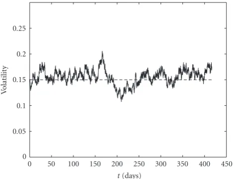
Figure 1: True constant volatility (dashed) versus its estimate (continuous).
electricity price observed each hour from the 1st of July 2000 to the 30th of June 2001 and the daily price of the Hang Seng index of the Hong Kong market from 1995 to 2007. It is worth noting that in all illustrative synthetic examples of this paragraph, the parameters can be chosen arbitrarily. The only essential thing to account for are realistic values of the volatility.
The proposed method is compared with the UKF for, first, the case of a periodic function of time, and second the case of a “synthetic” stochastic process. UKF is based on a state which has the unobservable volatility process as one of its components. UKF equations of the time and
mea-surement updates for the first momentμof the conditional
density are, respectively,
μ(ti+1|ti)=μ(ti|ti) +E(Fi)(ti+1−ti),
μ(ti+1|ti+1)=μ(ti+1|ti),
(11)
Estanding for the mathematical expectation. UKF, thus,
does not update prior estimatesμ(ti+1|ti), and consequently
it is not able to track time-varying volatility. Similar behavior
is exhibited in [10,11].
Next, a comparison is made between the above method
and an offline estimation of the volatility. The latter was
proposed in [12] which deals with the construction of a
black-box continuous time model for the squared volatility
process in the form of a stochastic differential equation.
The starting point in this construction is a parametric form for the covariance function of this process. The model frame derives from a control theory technique known as the shaping filter. We give a brief account of the work presented
in [12] and show that our present study outperforms it.
As regards observations, they are made according to both periodic and nonperiodic sampling schemes. For instance,
the case of jitter sampling, as in [15], is considered in
Section 3.2. The obtained performance is as good as that of a periodic sampling scheme.
0.05 0.1 0.15 0.2 0.25 0.3
V
o
latilit
y
0 50 100 150 200 250 300 350 400 450
t(days)
Figure2: True volatility (dashed) versus its estimate (continuous).
3.1. Constant volatility
The observations are simulated with a volatility of 0.15. The initial value of the volatility, in the proposed method,
is deliberately taken equal to the true value (= 0.15) so
that we evaluate the residual estimation error. A periodic sampling scheme has been used. The result is reported in
Figure 1. Both the mean value and the standard deviation of the relative error of estimation are about 1% and 6%, respectively. They are calculated by time averaging since the volatility value is constant along its trajec-tory.
3.2. Volatility as a step function
In order to illustrate the convergence behavior of the proposed method, a step function with the initial value
of 0.1 and the final value of 0.2 is taken as the volatility
sample path. The proposed method is implemented with
an initial value of 0.1 for the volatility. A jitter sampling
scheme has been used with maximum value of half the sampling period. Many simulations have been carried out
with different values ofλ; the value 0.04 forλmakes a good
tradeoffbetween robustness and right track. The result is
reported inFigure 2; it shows the capability of the algorithm
to follow rapid variations even for nonuniformly sampled data. Both the mean value and the standard deviation of the relative error of estimation are about 1% and 10%, respectively. Here again they are calculated by time averaging; this is legitimate since there is piecewise repetition of the volatility value along its trajectory. To explore further the performance evaluation of this result, we have computed
the Theil index. It is approximately 3·10−5. The Theil index
formula is
Theil= 1
N
samples σest σreflog
σest σref
0.05 0.1 0.15 0.2 0.25 0.3
M
ean
value
o
f
the
vo
latilit
y
0 50 100 150 200 250 300 350 400 450
t(days)
Figure3: True volatility (dashed) versus the mean for 100 of its estimates (continuous).
HereNis the number of samples in the reference trajectory
to be estimated. σest is the estimate of the volatility σt
at t=ti+1, denoted byσi+1 in Section 2, and σref is the
reference: the (true) volatility σt at t = ti+1, denoted
σi+1 (i=0,. . .,N−1).
In addition, Monte Carlo simulations have been carried out: the mean sample path for 100 estimated trajectories of
the volatility is reported in Figure 3. The mean value and
the standard deviation of its relative error of estimation are about 1% and 5%, respectively. This shows that the standard deviation of the estimation error drops significantly as the simulation number increases. That is, as expected, the empirical mean sample paths are to converge to the true mean.
As has been said in the introduction to Section 3,
the parameters can be chosen arbitrarily within all syn-thetic examples. The only essential thing to take into consideration is the realistic values of the volatility. The general validity of our method should thus be studied by varying these parameters. They are the initial and the final values of the step function in the context of
this subsection. Column 1 in Table 1 shows initial values
of three different step functions; column 2 shows their
corresponding final values. Columns 3 and 4 show the mean value and the standard deviation of the relative error of estimation obtained by Monte Carlo simulations (25 estimated trajectories of the volatility for each couple of parameters). The last two columns show the mean Theil index of the 25 estimated trajectories of the volatility using our method versus the Theil index of UKF for each couple of parameters.
3.3. Volatility as a deterministic periodic function of time
Whenever the volatility is subject to seasonality, we wish to recover the season(s) using our method. We consider the following deterministic function of time for the volatility
0.05 0.1 0.15 0.2 0.25 0.3
V
o
latilit
y
0 1 2 3 4 5 6 7 8
t(days)
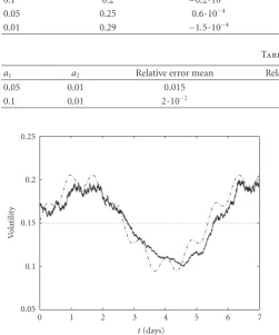
Figure 4: True (dashed) versus estimated volatility: proposed method (continuous), UKF (dotted).
trajectory:
σ(t)=a0+a1sin(ω1t) +a2sin(ω2t). (13)
The pulsations ω1 andω2 correspond to a one-week and
a one-day seasonality; this is, for instance, the case of
German electricity price treated in 3.6. a0, a1 and a2 are
chosen so as to have realistic values of the volatility. In
the simulation of Figure 4, they are 0.15, 0.05, and 0.01,
respectively.
Both the true volatility and its estimate for a periodic
sampling scheme, and forλof 0.07, are plotted inFigure 4.
The estimated volatility using UKF is constant, yet the proposed method is able to track the volatility oscillations.
The Theil index is about 10−3; UKF yields a Theil index
of 10−2. The mean value and the standard deviation of the
relative error are about 1% and 16%, respectively; they are calculated by time averaging. To justify this, we do check error ergodicity. This is done by fixing an instant, repeating again the simulation several times with respect to the same volatility trajectory till this instant. The mean value and the standard deviation of the relative error for this instant are obtained by averaging on simulations. Their values are in the order of what is given above. Besides, we proceed likewise in the following (the mean value and the standard deviation of the relative error are to be calculated by time averaging).
The mean trajectory of 100 estimated trajectories of the
volatility is reported in Figure 5. The mean value and the
standard deviation of its relative error of estimation are about 1% and 8%, respectively. In addition, the power spectral densities (PSD) for the true volatility sample path and the
mean of its estimates are confronted in Figure 6; the two
PSDs therein are clearly close to each other.
We furthermore vary the parameters a1 and a2 and
perform Monte Carlo simulations (100 estimated trajectories of the volatility for each couple of parameters) so that we
Table1
Initial value Final value Relative error mean Relative error StD Theil index Theil index UKF
0.1 0.2 −0.2·10−5 0.05 2·10−3 0.2
0.05 0.25 0.6·10−4 0.1 4·10−2 1.49
0.01 0.29 −1.5·10−4 0.06 1.5·10−2 20
Table2
a1 a2 Relative error mean Relative error StD Theil index Theil index UKF
0.05 0.01 0.015 0.08 10−4 3·10−2
0.1 0.01 2·10−2 0.1 2·10−3 0.4
0.05 0.1 0.15 0.2 0.25
V
o
latilit
y
0 1 2 3 4 5 6 7
t(days)
Figure5: True volatility (dashed) versus the mean for 100 of its estimates (continuous).
3.4. Volatility as a stochastic process
To synthesize sample paths of the volatility process as well as the stock price, the following SDE of Vasicek is considered:
dσt=α(θ−σt)dt+ξdBt, (14)
whereα=0.0001, θ=0.15, andξ=0.0007. We assume the
driftμis known (μ=0.015). The true volatility sample path
and the estimated one, using both the proposed method and
UKF, are reported inFigure 7. The volatility is estimated at
every half hour for 416 days. For this simulation, we choose
the initial value of the volatility equal toθ(=0.15). As above,
the estimated volatility using UKF is constant. The proposed method, however, is able to track the volatility fluctuations.
The empirical distribution of the estimation error for the
sample path in Figure 7is reported inFigure 8. Like UKF,
the proposed method is subject to bias, but the bias is clearly
smaller. The standard deviation obtained with UKF is 0.033,
whereas within the proposed method, it is 0.015.
3.5. Illustration using real data
Figure 9 shows the daily price of the Hang Seng index of the Hong Kong market from 1995 to 2007. This sample
0 0.1 0.2 0.3 0.4 0.5 0.6 0.7 0.8 0.9 1
M
ag
nitude
0 0.2 0.4 0.6 0.8 1 1.2 1.4 1.6 1.8
×10−3 Reduced frequency
Figure6: PSD of the true volatility (continuous) and that of its estimate (dotted).
path exhibits a volatility clustering phenomenon: periods of high-price fluctuations are followed by periods of high fluctuations, and the same can be said about periods of low-price fluctuations. The implementation result on this sample
path is shown inFigure 10. Notice the beginning of a period
of high volatility around the 700th day; this corresponds to the Asian financial crisis of October 1997.
3.6. Comparison with offline estimation of the volatility
We assume prior information about the unknown process
(σt)2: its stationarity in the large sense and a parametric
model for its covariance function. Let the covariance
func-tion of the process (σt)2be given by the following formula:
k(τ)=De−α|τ| α >0, (15)
where D is the process variance. This type of covariance
function allows one to fit the observed time dependence in the returns. Such a covariance function includes memory in the correlation pattern of the volatility. The spectral density
of (σt)2is then given by the formula
s(ω)= 1
2π
2Dα
0.06 0.08 0.1 0.12 0.14 0.16 0.18 0.2 0.22 0.24 0.26
V
o
latilit
y
0 50 100 150 200 250 300 350 400 450
t(days)
Figure 7: True (continuous) versus estimated volatility sample path: proposed method (dotted), UKF (dashed).
0 500 1000 1500
−0.1 −0.06 −0.02 0.02 0.06 0.1 (a)
0 500 1000 1500
−0.1 −0.06 −0.02 0.02 0.06 0.1 (b)
Figure8: Empirical distribution for the estimation error. (a) The proposed method, (b) UKF.
The spectral densitys(ω) is rewritten as
s(ω)= 1
2π
HF((jωjω))2, ω∈R, (17)
where
H(jω)=2Dα, F(jω)=jω+α. (18)
Now
Φ(s)=H(s)
F(s), s∈C, (19)
represents the transfer function of a stationary linear system;
the system is, furthermore, stable as the root of F(s) is in
the left half-plane of the complex variables. Recalling that
1/2πis the spectral density of a white noise of intensity 1, we
8.8 9 9.2 9.4 9.6 9.8 10 10.2 10.4
0 500 1000 1500 2000 2500 3000 3500
t(days) Signal
Figure9: Log-price of the Hang Seng index.
0.165 0.17 0.175 0.18
V
o
latilit
y
0 500 1000 1500 2000 2500 3000 3500
t(days)
Figure10: Estimated volatility sample path.
come to the following conclusion. (σt)2may be considered
as the response of the filter whose transfer function isΦ(s)
to a white noise with unit intensity. From the ordinary
differential equation describing such a filter, we obtain the
following stochastic differential equation as a model for
the squared volatility process (σt)2. This is the first state
component denoted byX1
t:
dX1
t =Xt2dt,
dXt2= −αXt1dt−
2DαdWt.
(20)
Here, W is a stochastic process with independent and
stationary increments of intensity 1. If we suppose that
W starts at 0 and that its trajectories are continuous in
probability, then we can give it the name L´evy process. We suppose further the existence of stationary solutions to the
−4
−2 0 2 4 6 8
0 50 100 150 200 250
t(days) Signal
Figure11: Log-price of the electricity.
0 5 10 15
0.04 0.06 0.08 0.1 0.12 0.14 0.16 0.18 0.2 0.22 (a)
0 50 100 150 200 250
0.04 0.06 0.08 0.1 0.12 0.14 0.16 0.18 0.2 0.22 (b)
Figure 12: Histograms of online volatility estimate (b) and an offline one (a).
positivity of Xt1. According to the above notation, (2) is
rewritten in the form
d yt=
μ−Xt1 2
dt+
X1
tdBt. (21)
We suppose that the condition in the proposition of
paragraph 4 of [12] applies, which ensures that (20) has
stationary solutions. We then calibrate the model (20
)-(21) on the observations from which seasonality has been
removed. The calibration is based upon stochastic calculus and the L´evy processes theory.
First, we apply the above offline method to electricity
price; observations of the German market for each hour from the 15th of June 2000 to the 31st of December 2003 are
processed.Figure 11shows the asset log-price trajectory. The
obtained varianceDand rateαamount to around 2.98·10−6
and 0.03, respectively.Figure 12displays two histograms: at
the top is the histogram of the sample path of the volatility process obtained from the above method, at the bottom is
0 1000 2000 3000
0.021 0.023 0.025 0.027 0.029 0.031 (a)
0 1000 2000 3000
0.021 0.023 0.025 0.027 0.029 0.031 (b)
0 1000 2000 3000
0.021 0.023 0.025 0.027 0.029 0.031 (c)
Figure13: Histogram of sample paths for the true volatility (a), histogram of the offline volatility estimate (b), and histogram of the online volatility estimate (c).
the histogram of the volatility sample path estimated by the main method of the paper. Second, since volatility is actually impossible to observe, showing only an application of the online method on real data is not ideal for a comparison with
the offline method of this subsection. We compare the two
methods on the synthetic stochastic process ofSection 3.4;
this is shown inFigure 13below.
4. CONCLUSION
Evidence to date suggests that stochastic volatility models for market prices are likely to be useful in practice. A real-time estimation algorithm of the volatility when observing the market asset price is proposed. The obtained estimate shows a clear improvement of precision when compared with the unscented Kalman filter. The proposed method inherits a low computational cost from LMS algorithms. Our algorithm has a complexity of 9 elementary operations per sample.
It outperforms the offline method inasmuch as it does not
require any effort to transform data, for example, to take
seasonality off. This, on the other hand, was necessary in the
method of the previous subsection.
REFERENCES
[1] F. Black and M. Scholes, “The pricing of options and corporate liabilities,”Journal of Political Economy, vol. 81, no. 3, pp. 637– 654, 1973.
[3] N. Shephard and T. Andersen, “Stochastic volatility: origins and overview,” inHandbook of Financial Time Series, Springer, New York, NY, USA, 2008.
[4] N. Shephard,Stochastic Volatility: Selected Readings, Oxford University Press, Oxford, UK, 2005.
[5] J. Hull and A. White, “The pricing of options on assets with stochastic volatilities,”The Journal of Finance, vol. 42, no. 2, pp. 281–300, 1987.
[6] E. M. Stein and J. C. Stein, “Stock price distributions with stochastic volatility: an analytic approach,” The Review of Financial Studies, vol. 4, no. 4, pp. 727–752, 1991.
[7] S. L. Heston, “A closed-form solution for options with stochastic volatility with applications to bond and currency options,”The Review of Financial Studies, vol. 6, no. 2, pp. 327– 343, 1993.
[8] A. H. Jazwinski, Stochastic Processes and Filtering Theory, Academic Press, New York, NY, USA, 1970.
[9] S. Julier and J. K. Uhlmann, “A new extension of the Kalman filter to nonlinear systems,” in Proceedings of the 11th International Symposium on Aerospace/Defense Sensing, Simulation and Control, Orlando, Fla, USA, April 1997. [10] H. Singer, “Continuous-discrete unscented Kalman filtering,”
http://www.fernuni-hagen.de/FBWIWI/forschung/beitraege/ pdf/dp384.pdf.
[11] O. Zoeter, A. Ypma, and T. Heskes, “Improved unscented Kalman smoothing for stock volatility estimation,” in Proceed-ings of 14th IEEE International Workshop on Machine Learning for Signal Processing (MLSP ’04), pp. 143–152, Sao Luis, Brazil, September-October 2004.
[12] H. Baili, “Uncertainty management for estimation in dynam-ical systems,” inProceedings of the IEEE Asia Pacific Conference on Circuits and Systems (APCCAS ’06), pp. 1992–1995, Singapore, December 2006.
[13] V. S. Pugachev and I. N. Sinitsyn,Stochastic Systems, Theory and Applications, John Wiley & Sons, New York, NY, USA, 1987.
[14] L. O. Chua and P. M. Lin, Computer-Aided Analysis of Electronic Circuits: Algorithms and Computational Techniques, Prentice-Hall, Englewood Cliffs, NJ, USA, 1975.
[15] E. Lahalle and J. Oksman, “LMS identification of CAR models,” inProceedings of the 5th International Conference on Information, Communications and Signal Processing, pp. 381– 384, Bangkok, Thailand, Decembre 2005.