Parameter Adjustment for a Dynamic Programming Track-before-Detect-Based Target Detection Algorithm

(1)

Volume 2008, Article ID 146925,19pages doi:10.1155/2008/146925

Research Article

Parameter Adjustment for a Dynamic Programming

Track-before-Detect-Based Target Detection Algorithm

O. Nichtern and S. R. Rotman

Department of Electro-Optics, Ben-Gurion University of the Negev, Beer-Sheva 84105, Israel

Correspondence should be addressed to O. Nichtern,[email protected]

Received 28 March 2007; Revised 13 November 2007; Accepted 29 January 2008

Recommended by Roy Streit

This paper addresses the problem of tracking a dim moving point target in a sequence of IR images. The proposed tracking system, based on the track-before-detect (TBD) approach, is designed to track and detect dim maneuvering targets from an image sequence under low SNR conditions; a dynamic programming algorithm (DPA) is used to process the frames in the sequence. This paper deals with the practical issues of setting the parameters of our algorithm to maximize tracking capability. In our flexible approach, we are able to accommodate different levels of noise and different target velocities and mobilities. Our algorithm is tested on real data to determine its efficacy.

Copyright © 2008 O. Nichtern and S. R. Rotman. This is an open access article distributed under the Creative Commons Attribution License, which permits unrestricted use, distribution, and reproduction in any medium, provided the original work is properly cited.

1. INTRODUCTION

The detection and tracking of point targets is necessary in many military applications. One particular use is in IRST (infrared search and track) systems where the data from the infrared spectra is used to detect targets which can be moving at subpixel velocities and subtend areas less than a pixel. Various researchers have developed track-before-detect (TBD) methods based on the dynamic programming algorithms (DPA) [1–5].

In the DPA approach, one continually incorporates new data (consisting of new infrared images or frames) into an estimate of where the targets may be. Each pixel is considered a potential target; a score is assigned to how target-like the pixel is. No attempt is made to continually decide definitely where the target is; that decision is made only when called upon or when the data ceases to flow. Hence this methodology is called track-before-detect.

In this paper, we will examine the practical problems involved in implementing a DPA on real data involving clouds in the sky (as clutter) and jet airplanes (as targets). We will note how practical examination of the data allows us to determine what the ratio between the reliability given to the new data compared to that associated with the accumulated score should be. Results will be shown on real data.

2. POINT TARGET DETECTION AND

TRACKING IN AN IR SEQUENCE

2.1. General architecture

The system performs target detection and tracking in three steps. The first step is whitening preprocess, which suppresses the clutter and emphasizes the target [6]. In this paper, we will assume that it is done by the simple antimedian filter where we subtract from each pixel an estimate based on the mean of the surrounding neighboring pixels. The second step is target detection and tracking based on the TBD approach and implemented using the DPA. The third step is the decision of the target presence and position after the last frame and retrieval of its trajectory. Currently, the pixel with the highest accumulated score in the last processed frame is selected as the target. Future research can involve the usage of a CFAR (constant false alarm rate) algorithm using known null hypothesis probabilities. The general system architecture is given inFigure 1; we concentrate in this paper on the DPA stage.

2.1.1. The target model

(2)

IR sequence

Whitening stage

DPA/TBD stage

Decision stage (could

be CFAR)

Target track

Figure1: Tracking system architecture.

spatial target signature, as projected onto the sensors array focal plane, is dominated by the optics point spread function (PSF). Being dependent on the range to the target and the aspects angle between the target and detector array, the target PSF is not constant. Still, the sampled target signature is often modeled as Gaussian:

S(x,y)=γ·e−1/2

x−x0

σx

2

+

_y₋_y 0

σy

2

, (1)

wherex0 and y0 are the possibly fractional targets’

coordi-nates (pixel coordicoordi-nates of the signature in the focal plane), γψ is the peak intensity at (x0,ψ y0), and σx2ψ and σy2ψ are the targets’ horizontal and vertical radiance variances, respectively [7,8]. Both the detected target radiation inten-sity and its PSF depend on the wavelength to which the detectors are sensitive, the target specifications, for example, as hot body tracking or plume tracking and the atmospheric transmission window (e.g., the 3–5 [μm] MWIR is often used for image target tracking systems).

2.1.2. IR background scene and atmospheric effects

The background of interest is composed of skies, either clear or cloudy. The sky primary source of radiation in the IR band is of course the sun. The amount of sun radiation that reaches the sensor array depends on the number of atmospheric layers the radiation pass through and the angle between the sun and the sensing system. For low sun angles or many atmospheric layers, less radiation will be collected by the sensors. Another major source of illumination is the sky light, which is scattered sun radiation but has diﬀerent spectral distribution (i.e., its peak is in the visible blue spectrum). Absorption is the most serious problem faced by IR systems and it actually defines the wavelength “window” at which IR systems work. Within these windows the received radiation is aﬀected by clouds and haze, fog and atmospheric gases such as ozone and carbon dioxide (although the later influence on the radiation within the near atmosphere is minimal). It is scattered away from the line of sight by aerosols suspended in the atmosphere and temperature changes along the radiation path can cause scintillation, which is a severe problem that IRST systems have to deal with, this phenomena occurs mostly near sea level. Fog and clouds are strong scatters and can be opaque to distant IR targets radiation. The presence and characteristics of fog, haze, and clouds depend on the geographic region, as well as on the season and altitude; hence fog is more probable in regions with high humidity, whereas dust can be expected in dry areas. There exist several computer models such as LOWTRAN (low spectral resolution) or MODTRAN

(moderate spectral resolution) that serve to model and forecast atmospheric conditions.

Although there exists no unique model for the IR sky background scene, many models assume a first-order Markov process and describe elevation and azimuth corre-lation to model cloud clutter analytically.

2.2. The DPA stage

An IR sequence containing background noise and clutter Section2.1.2, and a subpixel maneuveringtarget are the bases of our data model (first-order hidden Markov model), where the target track is the hidden sequence of events, and the IR sequence frames are the observed data. Barniv [9,10] has suggested a method for using the DPA in target tracking, which was further developed by Arnold [11], to allow tracking where nonwhite Gaussian noise (WGN) is present. The algorithm presented in this paper further develops the ideas presented in [2–4].

The DPA aids in the tracking of a dim point target maneuvering in a noisy background. The noise is assumed to be temporally and spatially uncorrelated (after the whitening stage); the target on the other hand moves in a smooth manner with only gradual changes in direction and speed. Deviations from either of these two assumptions will degrade the eventual system performance.

The algorithm processes a batch of frames rather than a single frame. In every frame, each pixel is given an accumulated score composed of its score in the present frame (after the whitening stage), and an accumulated score of the previous frames. The score is calculated using an accumulated score function (ASF) which will be introduced in Section 2.2.1. These accumulated scores of the pixels in the processed batch, as well as the calculated direction Section 2.2.3of the pixels are stored in theaccumulated score matrix(ASM) for every processed frame.

During the processing of the batch frames, a calculation is made to find the origin of each pixel within the previous frame thus forming atracking matrixSection 2.2.4, and the estimated direction of the target Section 2.2.3. At the last processed batch frame, a pixel with the highest accumulated score is assumed to be the target, and using the tracking matrix, its trajectory is found by backward calculation Section 2.2.4.

2.2.1. Accumulated score matrix

(3)

The ASF is composed of three components: (1) pixel score in the current whitened frame (WF), and (2) and (3) are two diﬀerent functions of the pixel’s accumulated score up to the previous frame, weighted by a parameterg. The two last components are both multiplied by a memory coeﬃcientb,determining the past information influence on the ASF of the current frame. The two last components take a valid search area, or matrix, from which the target may have arrived from in the previous frame. The first method, called the max method, orα(x,y), takes the maximum of the ASF elements within the valid search area. The second method, called sum method, orβ(x,y), takes the summation of the ASF elements within the valid search area.

For clear tracks, the maximum value (1st method, maximum) will allow an accurate evaluation of the track; when the target is very weak, tracking can be done through the tacking of the overall cloud being produced (2nd method, summation) rather than the maximum value from a single target. By combining and weighting these two approaches, coverage of all the possibilities might be achieved. This is an extension to the classic DPA where the evolution of the system is done using optimization alone, that is, always choosing the maximum value. The ASF is calculated as follows:

ASFn(x,y)=WFn(x,y)+b·g·α(x,y)+(1−g)·β(x,y). (2)

We will assume that the target velocity is within the range of 0–2 [ppf] (pixels per frame) and a possible jitter of 0.5 [ppf]; thus, the pixel can move up to 2.5 [ppf] in the horizontal and vertical directions; hence a valid search areaγ, from which a pixel might originate from in the previous frame is a 7×7 matrix. Given the target model above,α(x,y) andβ(x,y) are defined as

α(x,y)≡ 3

i,j=−3γ

(x,y)_i_,_j,

β(x,y)≡max γ(x,y)_i_,_j

i,j=−3,...,3,

(3)

where γ holds the valid search area elements ASF of the previous frame:

γ(x,y)_i_,_j=ASFn−1(i+x,j+y). (4)

2.2.2. The probability matrix W

In (4),γ(x,y)i,j the ASF values of the previous frame were taken. Since the pixels in the valid search area have diﬀerent probabilities of being the target in the previous frame, the ASF values of the previous frame can be multiplied by a weighting matrix that will take into account unreasonable changes in direction and velocity, and the sensor jitter. The following paragraphs will elaborate on the matter.

Since the target radiation spreads over several adjacent states (pixels), we are actually looking for the progress of this group of pixels. As mentioned in Section 2.2.1, the radiation spread is defined by the target’s signature that is related to its shape and movement parameters as velocity

and trajectory, by the sensor parameters as its sensitivity and integration time and by the platform jitter and movement. Since we are looking for the progress of a group of pixels, it is natural to combine their total energy into the score function, thus tracking the pixel to which the total contribution was maximal. Since not all of the contributing pixels have the same probability to be the main source of energy to the examined pixel, their position is assigned with a weighted factor according to the velocity/jitter/sensor PSF assumptions.

This point can be clarified by the following 1D example: consider a subpixel size target that captures a quarter of the pixel FOV moves horizontally at 0.25 pixels per frame and is captured by a platform whose jitter distribution is estimated to be horizontal with U [−1, +1] (uniform PDF over the range of−1 to +1 pixels). Because of uncertainty in the targets’ origin, it can be captured by either the same pixel, with probability of 3/4; or by the next adjacent pixel, with probability of 1/4. Because of the sensor jitter, each pixel can capture either its former FOV or, at most, one of its horizontally adjacent FOVs. Therefore, the origin of the current target can be any one of four diﬀerent pixels in the former frame, each with a diﬀerent probability. Now consider a 1 by 3 Gaussian target. This adds to the number of possible origins two more positions, one to each horizontal side, resulting in total of 6 possible origins. An introduction to the subpixel detection problem is presented in [12].

Since the probability of the jitter and the probability of position due to velocity are independent, the overall position probability is the product of these two probabilities. Marking the position probability due to jitter (pj) of the pixel in theθ location, and in thekth frame by pj(θk), and the position probability due to target motion by pv(θk) the weight is providedwv(θk)= pv(θk)·pj(θk).For the (k+ 1)th frame, the group of weights for former possible pixels from which a pixel might have originated is denoted by{wv(θk)},i ∈Ω; where Ω is the valid search area in the kth frame. Ω is a moving window, and its size is determined by the maximum allowed velocity plus the maximum shift due to the jitter. The jitter is a remnant of the imperfectly registered raw data at the input, which we assume to be given.

As mentioned in Section 1, the requirement to detect distant targets moving at subpixel velocities rationalizes the straight motion assumption. For 1D movement the set of probabilities {wv,i,k} is a vector; the expansion to a 2D motion is straightforward, either by using the notation of Arnold and Barniv and dividing each observation into numerous cells, each representing data of a particular axis; or by computing a 2D set of probabilities{wv,i,k}; that is, let{wv,i,k}be a matrix.

In our implementation, the valid search area will define a probability matrix W which contains the probabilities of pixels in the previous frames being the origin of the pixel in the current frame. The probability matrix is a superposition of two matrices—(1) a basic matrixWbasicand

(2) a penalty matrixWPenalty. The superposition is weighted

by a parameterp.

Wbasicincludes the eﬀect of Gaussian target spread and

(4)

9 8 7 6 5 4 3

10 9 7.5 6 4.5 3 2

11 10 9 6 3 1.5 1

12 12 12 12 0 0 0

11 10 9 6 3 1.5 1

10 9 7.5 6 4.5 3 2

9 8 7 6 5 4 3

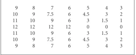
Figure 2: 7×7 penalty matrix WPenalty(direction = 1) in the

estimated direction→(0◦).

in place; the second matrix WPenalty(direction) gives high

probability to pixels in an assumed direction from which a target might have originated, and lower probabilities as the pixels vary from the assumed direction of arrival. Estimation of the movement in the current frame is discussed later in direction calculationSection 2.2.3.

We will assume a sensor jitter of U [−0.5, +0.5] (uniform PDF over the range of−0.5 to +0.5 pixels), and a Gaussian target spread of 3×3. In our caseWbasicelements,wbasic,i,j,

hold the probabilitiespj(θk) discussed above.

Instead of using the suggestedpj(θk) elements inWPenalty,

we use diﬀerent implementations. WPenalty(direction) gives

small penalties for small turns and severely decrease the score for sharp turns. Succary et al. [2] suggested using a penalty parameter that increases as the turn angle increases. Using that method, a turn of 45 degrees leads to penalty of–x, 90 degrees to−2x, and so on. The parameter value used was found by empirical. The angles are symmetrical with respect to the axis of assumed direction.Figure 2shows the 7×7 penalty matrixWPenalty(→)(0◦). We have takenx = 3. The

estimated region of arrival gets the highest values, 12 in this case. The values decrease until reaching the cells opposite to the estimated direction. There is a tradeoﬀbetween the need for penalty on change of direction and the need for adaptation to maneuvering targets.

The element values of the 7×7WPenalty(direction) matrix

are normalized to probabilities using the denominator in (5). The matrix is then multiplied by theWframematrix which

is used to adapt the penalty matrix to the assumed range of velocities by zeroing out all penalty pixels not contained in Ω(the valid search area in thekth frame) and keeping pixels withinΩ. HenceWframeis 1 withinΩand 0 otherwise.

There are nine diﬀerent probability matrices for each of the possible assumed directions: 0◦–315◦ at steps of 45◦ (directions 1–8, resp.), and remaining in place (direction 9). The probability matrix is given as

W(direction)

=p·Wbasic+ (1−p)·

WPenalty(direction)·Wframe

i,jwPenalty(direction)i,j·wframe;i,j. (5)

Figure 3shows the basic probability matrix (direction 9), the eight penaltymatrices for the diﬀerent directions (direction 1–8), and the resulting nine probability matrices. The basic probability matrix incorporates the allowed jitter and represents a standing target. InFigure 3, the target is assumed

to be at a velocity range of 0-1 [ppf]; thus only a 5×5 matrix is needed (including the assumed jitter) and the border pixels are zeroes accordingly usingWframe. Thepparameter was set

to 0.5, giving equal weight toWbasicandWPenalty(direction).

All matrices are normalized to values between 0-1.

Equation (4) can be rewritten to contain the probability matrix:

γ(x,y)_i_,_j≡w(direction)i,j·ASFn−1(i+x,j+y), (6)

wherew(direction)i,j is the (i,j) element in the probability matrix,W.

2.2.3. Direction calculation

To use W(direction), the direction from which a pixel originated has to be found. We must now decide where it is most likely that the target previously was when moving in this particular direction. Estimation of the direction is based on (1) ASF, (2) the basic probability matrix (Wbasic), and (3)

direction consistency.

The calculation of the direction starts by creating a temporary 7 ×7 matrix (given our assumption of target velocity and sensor jitter). The previous frame ASFs as well as the directions of pixels in the area of 7×7 are retrieved from the ASM. Each pixel is given a parameter Var that gets a value according to the pixel’s direction in the previous frame and its direction relative to the pixel under investigation (central pixel, Figure 4 shows the division of the 7× 7 matrix into the eight different directions, direction 1–8). The parameter gives maximal value for identical directions (direction consistency) and minimal value for opposite directions (direction inconsistency). No direction difference sets Var = 6, and every increase of 45 degrees difference lowers the value of Var by 1 (down to a value of 2 for 180 degree difference). The final score of each pixel in the temporary matrix is defined as

Source Pixel Score(x+i,y+j)

=ASFn−1(x+i,y+j)·wbasic;i,j·Var(i,j),

(7)

where ASFn−1(x+i,y+ j) is the pixel’s accumulated score

from the previous frame, wbasic,i,j is the value of Wbasic at

the (i,j) coordinate, and Var(i,j) is the direction diﬀerence parameter for the (i,j) coordinate.

The pixel with the highest score is chosen as the “source pixel.” Since each group of pixels in the matrix belongs to a specific direction, the direction in the current frame is now known and is saved in the ASM. In conclusion, to calculate the pixel’s direction:

(i) create a 7×7 temporary matrix;

(ii) find the direction of the pixels in the previous frame; (iii) calculate Var according to the direction consistency; (iv) calculate the temporary matrix score, source pixel

score (x+i,y+j);

(v) find the pixel with the highest score, and deduce the direction.

2.2.4. The tracking matrix

(5)

(a)

0◦ 45◦ 90◦

135◦ 180◦ 225◦

270◦ 315◦

6 4 2

2 4 6

6 4 2

2 4 6

6 4 2

2 4 6 6 4 2

2 4 6

6 4 2

2 4 6 6 4 2

2 4 6 6

4 2

2 4 6 6

4 2

2 4 6

(b)

0◦ 45◦ 90◦

135◦ 180◦ 225◦

270◦ 315◦ In place

2 4 6 6

4 2

2 4 6 6

4 2

2 4 6 6

4 2

2 4 6 6

4 2

2 4 6 6

4 2

2 4 6 6

4 2

2 4 6 6

4 2

2 4 6 6

4 2

2 4 6 6

4 2

(c)

Figure3: Probability matrices for the various directions. (a) The 7×7Wbasicmatrix, (b) the eight 7×7WPenaltymatrices for the diﬀerent

directions, after usingWframe, and (c) the nineW(direction) matrices forpset to 0.5, and velocity range [0-1] [ppf].

Direction 1-0 degrees Direction 3-90 degrees Direction 5-180 degrees Direction 7-270 degrees

Direction 2-45 degrees Direction 4-135 degrees Direction 6-225 degrees Direction 8-315 degrees

Figure4: The pixel groups belonging to each of the possible eight directions. The arrow points to the central pixel of the 7×7 matrix, and shows the direction of the pixels from the previous frame to the current frame.

previous Sections 2.2.2, 2.2.3. The origin is calculated by taking the element having the maximum value in (7):

i,j_x_,_y=max Source Pixel Score(x+i,y+j). (8)

The index of that pixel of origin is saved in the tracking matrix, in the [index, frame] element, where index represents the index of the pixel under investigation in the current frame, and frame is the value of the current frame. Given an image frame or a block the size ofN columns andMrows, index=(N−1)·M+M.

In that way, the DPA builds the tracks which are most probable of being the target’s track. At the last frame processed, the pixel with the highest score is picked, and the index of its pixel of origin from the previous frame is taken. At the previous frame, the found index is used to retrieve the origin of that index. That procedure is iterated down to frame 2.Figure 5shows a “target” found at index =578 in

frame 15. Tracking it back leads to index=470 in frame 14 and so on.

2.2.5. Parameter summary

In the previous sections, several parameters that control the algorithm functionality were introduced. These parameters are of high significance since they allow flexibility in the algorithm to eventually track and detect targets in an optimal fashion. A summary of the parameters is used inTable 2.

We will concentrate our paper on finding and evaluating the influence of b, and g on the algorithm. We assume a probability matrix weighting ofp=0.5 to allow for a certain amount of target maneuvering.

(6)

Index of maximal accumulative

score Frames

In

d

ex

es

1 · · ·

54 · · · 157 158 159 · · · 278 · · · 322 · · · 470 · · · 578 · · · 900

1 2 3 · · · 9 10 11 12 13 14 15

25 54

155 157

158 159

278 322

470

98 187 762

215

73

65 115

123

167 259 560

109 192 427

480 320

176

Figure5: Example of a tracking matrix, and the “target” track.

Table1: The various real IR sequences used for the testing.

IR sequence name IR sequence scene description Target(s) starting location [y,x] Target(s) velocity [ppf]

NPA Two targets in wispy clouds [49, 99], [160, 240] ≈0.2

NA23 Single fast target in bright clouds [136, 128] ≈0.3

Table2: Summary of EMCs for which tracking occurred in the IR sequences.

IR sequence name

Relevant range ofb’s

IR sequence name Relevant range ofs n Maximal target peak

([13, page 74])

where tracking occurred where tracking occurred

max part (g=0)

sum part (g=1)

max part (g=0)

sum part (g=1)

max part (g=0)

NPA ∼30 2–4.8 0–0.8 3 1 3–5 3–5

NA23 ∼60 4.4–4.6 0.2–0.8 3 1 1–5 1–5

Table3

b — The memory persistence coeﬃcient, determining the influence of the accumulated score.

p(and (1−p)) — The_on_{W(direction) probability matrix.}Wbasic(WPenalty(direction)) coeﬃcient determining the influence of the 7×7Wbasic(WPenalty(direction)) matrix

g(1−g) — The sum coeﬃcient determining the amount of influence of the summation (maximum) on the accumulated score.

2.2.6. The effective memory coefficient (EMC)

As can be seen from the (2), b determines the memory persistency or the decaying influence of the scores from the previously processed frames. To prevent the algorithm from “exploding” (i.e., exponentially increasing rather than decreasing), aneffective memory coefficient(EMC) has to be within the range of values 0-1. The EMC is introduced due to the fact thatbitself is not the memory coefficient, since it is multiplied by g or (1−g). The smallerb is, the less effect the previous frames have on the current score and the

(7)

g

0 0.1 0.2 0.3 0.4 0.5 0.6 0.7 0.8 0.9 1

b

0 1 2 3 4 5 6 7 8

Direction 1-8 Direction 9

Figure6: bversus gfor the direction 1–8 (solid blue line) and

direction 9 (dashed line) the black circles represent theg=0/1 cases and the equivalentbvalues.

coeﬃcient was obtained,b=0.7; on the basis of more recent research, we recommendb =0.8. The formula used for the accumulated score was

ASFn=WFn+b·max w·ASFn−1

(9)

and the normalization,

b= 0.8

max{w} (10)

was used in order to limitbto 0≤b≤1, and to maximize it for best performance.

The score formula in the current DPA version is

ASFn

=WFn+b·g·sum w·ASFn−1

+(1−g)·max w·ASFn−1

. (11)

Similarly, the requirement here is

b= 0.8

g·sum{w}+ (1−g)·max{w}. (12)

By the substitution ofg=0,g=1 case into the requirement, the following is obtained:

bg=0= 0.8

max{w}, bg=1=

0.8

sum{w}. (13)

It should be noted thatbg=0andbg=1are constant and

direc-tion dependent since they are derived from the probability matrices mentioned inSection 2.2.2.

After rearrangement, the following formula for EMC is derived:

b=

_g_·

sum{w}+ (1−g)·max{w}

0.8

−1

=g·b−1

g=1+ (1−g)·b−g=10 −1

(14)

Using the probability matrices achieved empirically Section 2.2.2, an appropriate range forbcan be found so that 0 ≤

EMC≤1. Putting that intobleads to

b=[1.118·g+ 0.131]−1 for direction 1 to 8,

b=[1.035·g+ 0.214]−1 for direction 9.

(15)

The derived formula suggests the values ofbthat should be used for a given value ofg. Since 0 ≤ g ≤ 1, a graph ofb versusgcan be plotted, as inFigure 6, and a valid range of values forbcan be found.

As can be seen from the graph, a valid range of values for bis about 0≤b≤8 forg=0 and 0≤b≤1 forg=1. Since bg=1 = 0.8 for all directions, memory values of around 0.8

should give the optimal performance forg=1, regardless of the scenery.Since the targets in the tested IR sequences move at subpixel velocities, mainly 0.2-0.3 [ppf], most of the time they are in direction 9 (standing in place); thus the algorithm is expected to be most eﬀective forbg=1=0.8andbg=0close to 4.65.

The graph above might also aid if a superposition of the sum and the max parts of the ASF are needed. Adjusting the superposition is done by simply assigningga value and deriving the appropriate value ofbfrom the graph. Finding the optimalbs (or range ofbs) for the diﬀerent scenes will be done by optimizing an algorithm score, given by a metric that will be defined inSection 2.3.

2.3. Performance metric

In order to evaluate the algorithm, the metric below has been defined. Each frame in the processed batch of frames is divided into blocks of sizeM×N(30×30 were used for slow targets, and 30×80 for fast targets). The algorithm is run over nine blocks, that is, the target block and eight adjacent blocks. The SNR of the target block (TB) and its eight adjacent nontarget blocks (NTBs) are calculated. Afterwards, an algorithm score is calculated based on the resulting SNRs (signal to noise ratios).

The block SNR is given as

Block SNR(i,j)=E

vi,j∈M

−Evi,j∈/M

σvi,j

, (16)

wherevi,jis the set of pixels belonging to the (i,j) block,Mis a set containing the five pixels with the highest scores in that block, andσis the standard deviation of the block pixels.

(8)

The algorithm score (A S) is given as

A S

=Block SNR(i,j){(i,j)}∈TB−E Block SNR(i,j)

{(i,j)}∈NTB

σ{Block SNR(i,j)}{(i,j)}∈NTB

.

(17)

The A S is calculated by subtracting between the TB’s SNR and the expectation value of the SNR of the NTB’s, divided by the standard deviation of the NTB’s SNR. The algorithm always identifies a target in each given block. Since that is the case, the false detection of targets should achieve less SNR in these NTBs than the true detection in the TB, resulting in a positive A S. It should be noted that the division to blocks is only for the purpose of algorithm evaluation (A S), whereas in real scenarios, the frames will not be divided. Also, only nine blocks were used due to memory and time complexity.

In the tests performed, other numbers of highest pixels, defined as Max Numbers, were taken to check the influence of the number of high pixels regarded as “target pixel” on theBlock SNR. Using the metric above for the A S, the EMC value for optimized algorithm work can be found, in both cases ofg=0 (the max part) andg=1 (the sum part) in the accumulated score of (2).

3. RESULTS

The DPA algorithm has been applied to several IR sequences containing different scenes and clutter degree. Each sequence contains 95 to 100 frames, and the algorithm ran on a batch of up to 25 frames. The results are shown for two IR sequences: NA23A and NPA. A single frame from the IR sequences showing the targets locations (in white rectangles) is shown inFigure 7. The NA23A sequence has a single target moving in clear sky from right to left atν≈0.3 [ppf]. The NPA sequence has two targets moving atν ≈0.2 [ppf]; the left target is engulfed in clouds moving from bottom to top, and the right target is moving in scarce clouds. The algorithm will be applied on the surroundings of the left target, since it is of more interest due to its more difficult condition. A target range velocity of 0-1 [ppf] has been assumed; hence 5×5 probability matrices were used.Table 1depicts the different IR sequences tested, the target(s) location, and the target(s) velocity.

The DPA was applied for two diﬀerent cases:g =0 (the maximum part in the ASF) andg =1 (the summation part in the ASF) over a range of values ofbto check the eﬀect of each part of the accumulated score formula on the algorithm results. The introduced metricSection 2.3was used to find the optimal values ofbs, for which tracking has occurred.

Afterwards, the effect of Max Numbers (the number of pixels with the highest scores considered to be “targe” in the Block SNR formula (16)) on the A S was checked. This action is taken to assure that the metric gives a reliable A S performance for the different EMCs (b), namely, selecting target affected pixels only as “target” pixels. Another aspect examined was the effect of the target velocity on the

(a)

(b)

Figure7: A single frame from IR sequences. (a) NA23A and (b)

NPA sequence showing the target’s locations (white rectangles).

algorithm performance by sampling the given IR sequences everys nframes, wheres nis a value in the range of 1 to 5.

Section 3is ordered as follows: (a) a preprocessing stage example is given for the NA23A sequence, (b) the NA23A and NPA sequence results are given, and (c) a brief summary of findings.

3.1. The preprocessing whitening stage

The algorithm starts by whitening the input IR sequence. According to the introduced A S metric, the sequence is divided into blocks. The TB and the eight surrounding NTBs are then whitened to reduce the clutter and emphasize the target, as can be seen in Figure 8 of the 1st frame of the NA23A sequence.

The process shown in Figure 8 is repeated for the required sequence frames before proceeding to the next stage of the DPA. (The frames can also be processed individually for a real-time implementation).

3.2. The DPA stage

(9)

250 200 150 100 50

50 100 150 200 250 300

400 600 800 1000 1200 1400 1600 1800 2000 2200

(a)

151 151.5 152 152.5 153 153.5 154 154.5 155 155.5 156

(b)

0 5 10 15 20 25

(c)

Figure8: Algorithm stages. (a) 1st frame of the original NA23A

sequence divided into blocks, (b) 1st frame of TB (target at center of frame), and (c) 1st frame of TB after the preprocessing whitening stage.

from pixel-to-pixel. If the target is moving at a subpixel velocity, these matrices are not used often and the algorithm will not perform at its peak. In order to find the velocity for which the algorithm worked best, the algorithm has been run over the sequence, in both cases ofg, fors nfrom 1 to 5, for example, givens n=5, take only every 5th frame.

b

0 1 2 3 4 5 6 7 8

Sc

o

re

−1 −0.5 0 0.5 1 1.5 2

Frame 25 Frame 24 Frame 23 Frame 22

Frame 21 Frame 20 Mean Median (a)

Frame: 25 Frame: 24 Frame: 23 Frame: 22 Frame: 21 Frame: 20

30 20 10

10 20 30 30

20 10

10 20 30 30 20 10

10 20 30 30

20 10

10 20 30 30

20 10

10 20 30 30 20 10

10 20 30

(b)

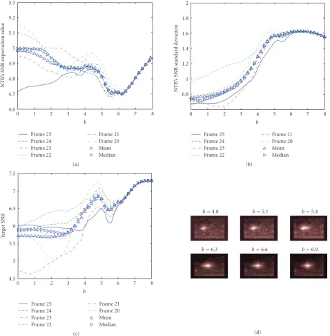
Figure 9: NA23A sequence preliminary results; g = 0,

Max Numbers=5. (a) A S forb=[0· · ·8], and six last frames; (b) the last six processed frames.

It should be noted that for the algorithm to accumulate eﬀectively, approximately 20 frames at minimum have to be processed, thus limiting the amount ofs nthat can be used depending on the number of available sequence frames.

To keep the target in the “target block,” a larger block size of 30×80 was used for fast targets instead of 30×30.

3.2.1. NA23A sequence

(1) Preliminary results(s n=1)

The results are first shown for the NA23A sequence,g =0 case. Figure 9shows the A S for the range of 0 ≤ b ≤ 8 at intervals of 0.2. The graph shows the A Ss for the last six frames, 20–25 in this case, for two reasons: (1) some frames might be noisier than the others; (2) we wish to show the accumulated score eﬀect.

The first cause will result in the target being dimmer compared to the clutter; the target may even disappear. In that case, the memory persistence and the accumulation of the score from frame to frame help maintain the track. The accumulated score helps overcome noisy frames, and “accumulates” the SNR for the dim target. Looking at the last frames helps us understand whether the eﬀect of accumulation is suﬃcient for the number of frames processed, or whether more frames need to be processed.

(10)

b

0 1 2 3 4 5 6 7 8

NTB

’s

S

NR

expec

tat

io

n

val

u

e

4.6 4.7 4.8 4.9 5 5.1 5.2 5.3

b

0 1 2 3 4 5 6 7 8

NTB

’s

S

NR

st

andar

d

dev

iat

io

n

0.8 1 1.2 1.4 1.6 1.8 2

Frame 21 Frame 20 Mean Median (b)

b

0 1 2 3 4 5 6 7 8

Ta

rg

et

S

N

R

4.5 5 5.5 6 6.5 7 7.5

Frame 21 Frame 20 Mean Median (c)

b=4.8 b=5.1 b=5.4

b=6.3 b=6.6 b=6.9

(d)

Figure10: NA23A sequence preliminary results;g=0, Max Numbers=5. (a) Standard deviation of NTB’s SNR, (b) expectation value of

NTB’s SNR, (c) TB’s SNR, and (d) last-processed frame (25th) for various values ofb.

The graph shows a peak at aroundb=4.8 for all frames. The rise at aboutb=6 is irrelevant since the algorithm was unable to track at EMC of about 6 or above. It can be seen that above that EMC, all the frames A S converge, suggesting that the EMC is too high and that the weight of the current frame is insignificant compared to the accumulated score. It seems that the relevant range for EMC can be narrowed to 0≤b≤6, for theb=0 case, in the current IR sequence.

A rise A S is expected as the frames advance. It can be seen in the graph inFigure 9(a), that the A S of the 20, 23 frames is lowest forb <3.5. That is due to the fact that these frames are noisy, as can be seen inFigure 9(b). Increasing the

EMC improves the A S of these frames, that is, more memory persistence and less weight to current noisy frame. Since the target moves atν≈0.3 [ppf] (stays in the same pixel most of the time) the expected theoretical peak (EMC calculation in Section 2.2.6) was at aroundb=4.65 in agreement with the results shown inFigure 9(a).

(11)

b

0 0.5 1 1.5 2 2.5 3 3.5 4 4.5 5

Sc

o

re

−1 −0.5

0 0.5 1 1.5 2

b

0 0.5 1 1.5 2 2.5 3 3.5 4 4.5 5

S

tandar

d

dev

iat

io

n

0.2 0.3 0.4 0.5 0.6 0.7 0.8 0.9 1 1.1 1.2

b

0 0.5 1 1.5 2 2.5 3 3.5 4 4.5 5

NTB

’s

S

NR

expec

tat

io

n

val

u

e

2 2.5 3 3.5 4 4.5 5 5.5

b

0 0.5 1 1.5 2 2.5 3 3.5 4 4.5 5

Ta

rg

et

S

N

R

1 2 3 4 5 6 7

Frame 21 Frame 20 Mean Median (d)

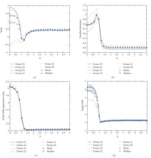
Figure11: NA23A sequence preliminary results;g=1, Max Numbers=5. (a) A S, (b) standard deviation of NTB’s SNR, (c) expectation

value of NTB’s SNR, and (d) TB’s SNR.

retained its high value (Figure 10(d)). Thus values of EMC higher than that will prevent the algorithm from tracking the target, since the trail pixels and the pixel of origin will gain a higher accumulated score, as will be seen later in Section 3.2.1(3).

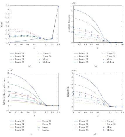
Results for theg =1 case are shown inFigure 11. As can be seen from the A S, the relevant range ofbis 0≤b ≤ 1, after which A S’s of the various frames converge regardless of the EMC. The TB’s SNR can be seen to fall at aroundb=1. The A S starts at its maximum (mean value) for no memory and drops as the EMC rises, untilb =1. This suggests that

in this case and for this particular sequence, the algorithm is not needed for the detection.

(12)

b=0 b=0.2 b=0.4 b=0.6 b=0.8 b=1

b=1.2 b=1.4 b=1.6 b=1.8 b=2 b=2.2

30 20 10

10 20 30 30

20 10

10 20 30

30 20 10

10 20 30 30

20 10

10 20 30

30 20 10

10 20 30 30

20 10

10 20 30

30 20 10

10 20 30 30

20 10

10 20 30 30

20 10

10 20 30

30 20 10

10 20 30 30

20 10

10 20 30 30

20 10

10 20 30

Figure12: Last processed frame (25th) forb=[0· · ·1].

them will also increase in their value, causing the ball to grow from frame to frame.

To conclude, a valid range of EMC, 0 ≤ b ≤ 8, has been found in which the algorithm is able to track and detect the target correctly; this concurs with the theoretical range. Section 3.2.1(2) will deal with the issue of target velocity, and will demonstrate that a preferred EMC exists, 0.6≤b≤0.8, close to the theoretical value.

(2) The s n variable

As stated in the beginning of Section 3.2, since the main advantage of the algorithm is the usage of the penalty matrices, the target has to move at a velocity of at least around 1 [ppf]. If the target in the sequence moves at lower velocities, ν ≈ 0.3 [ppf] in our case, the penalty matrices are used only every three frames roughly. Since that is the case, sampling of the sequence has been suggested, so that the target moves at higher speed. The first simulation was done fors n=4 (only every 4th frame was taken) giving the target a velocity ofν ≈1.2 [ppf]. To keep the target in the “target bloc,” a larger block size of 30×80 was used instead of 30×30.

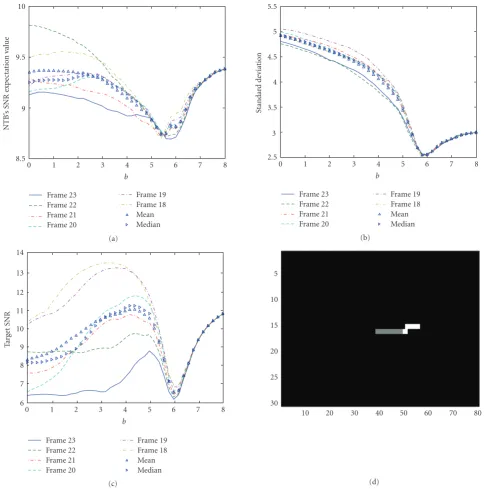
The A S and the last six frames are shown inFigure 13, for theg = 0 case. The A S achieved is lower in this case due to the noisy frames compared to the last six frames in thes n = 1 case. It should be noted that by sampling the sequence of the algorithm, different frames were processed that differ in their noise degree. Nevertheless, the A S shows the effect of accumulation as the frames progress the peak is distinguishable (above frame 20), and is aroundb =5.0 for the last three frames. An increase in the EMC is expected since the target now moves faster. It seems that the algorithm needs around 20 frames for the dim point target to accumu-late enough SNR to be distinguishable from the clutter.

Figure 14shows the graphs of the standard deviation of the NTB, the expectation value of the NTB SNR, the TB’s SNR (all versusb), and the target track found for s n = 4 (the pink portion of the track is the target track fors n=1). ComparingFigure 10toFigure 14shows that the TB and NTB SNRs behave similarly fors n=1 and fors n=4; only the TB SNR has a distinguishable peak. This shows that the penalty matrices help distinguish between target and clutter, and that the algorithm needs targets at aroundν ≈1 [ppf] to work eﬀectively. In the case ofg = 1, the A S is lower compared to the one achieved fors n =1, due to the noisy

b

0 1 2 3 4 5 6 7 8

Sc

o

re

−1.5 −1 −0.5 0 0.5 1 1.5

Frame=18 Frame=19 Frame=20 Frame=21 Frame=22 Frame=23

30 20 10

20 40 60 80 30

20 10

20 40 60 80 30 20 10

20 40 60 80 30

20 10

20 40 60 80 30 20 10

20 40 60 80 (b)

Figure 13: NA23A sequence,s n = 4. (a) The A S forg = 0,

Max Numbers = 5,b = [0· · ·8], and the six last frames, (b) images of the six last frames after the DPA algorithm.

last frames, as in theg =0 case.Section 3.2.1(3) deals with the issue of using values of the Max Numbers parameter that will correctly take only target pixels as the highest pixels.

(3) Finding Max Numbers

(13)

b

0 1 2 3 4 5 6 7 8

NTB

’s

S

NR

expec

tat

io

n

val

u

e

8.5 9 9.5 10

b

0 1 2 3 4 5 6 7 8

S

tandar

d

dev

iat

io

n

2.5 3 3.5 4 4.5 5 5.5

b

0 1 2 3 4 5 6 7 8

Ta

rg

et

S

N

R

6 7 8 9 10 11 12 13 14

30 25 20 15 10 5

10 20 30 40 50 60 70 80

(d)

Figure14: NA23A sequence,s n=4. (a) Standard deviation of NTB’s SNR, (b) expectation value of NTB’s SNR, (c) TB’s SNR, and (d) the

target’s track (the pink track is the target track fors n=1).

the figure for Max Numbers > 3. The result suggests that Max Numbers=3 is preferable for theg=0 case.

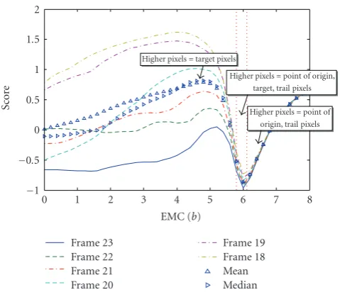
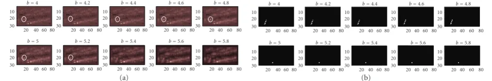
Figure 16shows the A S versusbof the NA23A sequence, for s n = 4. The graph is separated to three sections according to the resulting highest pixels in the last frame: (1) target pixels, (2) trail and target pixels and pixel of origin, and (3) pixel of origin and trail pixels. In the case of the 5 highest pixels, the A S takes only the target pixels up to b = 5.6 (as can be seen inFigure 17(a)). Above that value the trail pixels start to accumulate higher scores than the target pixels, until the pixel of origin also accumulates a higher score (b=

6.0). In the case of 3 highest pixels, the score takes only the

target pixels up tob=5.8 (as can be seen inFigure 17(b)). Higher EMCs cause nontarget pixels to be higher than the target pixels as before. In this case ofg = 0 and s n = 4, the algorithm was able to track and locate the target up to b = 6.0. Using that andFigure 16leads to the conclusion that a good range of EMCs would be 4.4≤b≤6. This range contains the theoretical EMC for nonmoving targets.

(14)

Max numbers

1 2 3 4 5 6 7 8 9 10

Sc

o

re

0.4 0.6 0.8 1 1.2 1.4 1.6 1.8 2 Frame 23 Frame 22 Frame 21 Frame 20 Frame 19 Mean Median (a) Max numbers

1 2 3 4 5 6 7 8 9 10

Ta rg et S N R 6 8 10 12 14 16 18 Frame 23 Frame 22 Frame 21 Frame 20 Frame 19 Mean Median (b)

Figure15: NA23A sequence,s n=4. (a) A S versus Max Numbers, (b) TB SNR versus Max Numbers.

EMC (b)

0 1 2 3 4 5 6 7 8

Sc

o

re

−1 −0.5 0 0.5 1 1.5 2 Frame 23 Frame 22 Frame 21 Frame 20 Frame 19 Frame 18 Mean Median

Higher pixels=target pixels

Higher pixels=point of origin, target, trail pixels

Higher pixels=point of origin, trail pixels

Figure 16: NA23A sequence,s n = 4, Max Numbers = 3, A S

versusb,g=0 case.

Figure 18 shows the detected target’s track. It can be clearly seen that up tob = 5.6 the tracking is reliable. An increase in the EMC causes inaccurate target tracking, where further increase (b > 6) causes previously target traversed pixels to achieve the highest accumulated score, and hence no tracking occurs.

The discussion continues now to theg=1 case. The last frames of the algorithm versusbare shown inFigure 19. It can be clearly seen that for 0≤b≤0.8 there is only one high pixel belonging to the target (surrounded by white circle). The algorithm tracks the target in the range of 0.2≤b≤0.8. These results suggest that Max Numbers=1 and 0.2≤b≤

0.8 should be used in the case ofg=1.

The A S using Max Numbers=1 is shown inFigure 20. A peak in the mean A S can be clearly seen for b = 0.6

b=4.4

b=5.2

b=6

b=4.6

b=5.4

b=6.2

b=4.8

b=5.6

b=5

b=5.8

30 20 10

20 40 60 80 30

20 10

20 40 60 80 30

20 10

20 40 60 80 30 20 10

20 40 60 80

30 20 10

20 40 60 80

30 20 10

20 40 60 80 30 20 10

20 40 60 80 30

20 10

20 40 60 8030 20 10

20 40 60 80

30 20 10

20 40 60 80

(a) b=4.4

b=5.2

b=6

b=4.6

b=5.4

b=6.2

b=4.8

b=5.6

b=5

b=5.8

30 20 10

20 40 60 80 30

20 10

20 40 60 80 30

20 10

20 40 60 80 30 20 10

20 40 60 80

30 20 10

20 40 60 80

30 20 10

20 40 60 80 30 20 10

20 40 60 80 30

20 10

20 40 60 8030 20 10

20 40 60 80

30 20 10

20 40 60 80

(b)

Figure 17: NA23A sequence,s n = 4, last processed frame. (a)

Highest 5 pixels emphasized and (b) highest 3 pixels emphasized.

(15)

b=4.4

b=5.2

b=6

b=4.6

b=5.4

b=6.2

b=4.8

b=5.6

b=5

b=5.8

30 20 10

20 40 60 80 30

20 10

20 40 60 80 30

20 10

20 40 60 80 30 20 10

20 40 60 80

30 20 10

20 40 60 80

30 20 10

20 40 60 80 30 20 10

20 40 60 80 30

20 10

20 40 60 8030 20 10

20 40 60 80

30 20 10

20 40 60 80

Figure18: NA23A sequence,s n=4, target’s track versusb.

b=0

b=0.8

b=0.2

b=1

b=0.4 b=0.6

30 20 10

20 40 60 80 30

20 10

20 40 60 8030 20 10

20 40 60 80

30 20 10

20 40 60 80 30 20 10

20 40 60 8030 20 10

20 40 60 80

Figure19: NA23A sequence,s n =4, last processed frame,g =

1 case, highest 5 pixels emphasized (target pixel surrounded by a white circle) versusb.

correct value of Max Numbers according to the case under investigation.

(4) Summary

Results of the NA23A sequence have been shown, with an emphasis on the eﬀect of the Max Numbers and the s n parameters. Preferable values for Max Numbers were found: Max Numbers=1 for theg =0 case, and Max Numbers=

1 forg = 1 case. Relevant ranges ofbs were also found for each case: 4.4 ≤ b ≤ 6 for theg = 0 case 0.2 ≤ b ≤ 0.8 for theg = 1 case. The g = 1 case has performed better for the faster target scenario (s n = 4). Once again, for each s nrate, the highest A S in the relevant ranges of bs was chosen. It should be noted that for the algorithm to accumulate effectively,at least 20 frames have to be processed, thus limiting the amount of sampling that can be done, depending on the number of available sequence frames. Also, different frames are processed for the different s ns, so a comparison might not be precise. The results are shown in Figure 21. The algorithm has a preferable target velocity at aroundν≈0.6±0.15 [ppf].

3.2.2. NPA Sequence

The sequence contains a target moving atν ≈ 0.2 [ppf] in the proximity of clouds. In this case, the cloud’s edges in the target block pose a challenge since they behave like targets and receive a high A S from the whitening preprocessing stage (source for clutter leakage). In this sequence, tracking and detection were achieved for s n ≥ 3. Hence detailed results for lowers nvalues will be skipped and only detailed

EMC (b)

0 1 2 3 4 5 6 7 8

Sc

o

re

−1 −0.5 0 0.5 1 1.5 2 2.5

Frame 19 Frame 18 Mean Median

Figure20: NA23A sequence,s n=4 A S versusb,g=1 case and

Max Numbers=1.

Sampling

0 1 2 3 4 5 6

Sc

o

re

−0.5 0 0.5 1 1.5 2

(a)

Sampling

0 1 2 3 4 5 6

Sc

o

re

0 0.5 1 1.5 2 2.5

(b)

Figure 21: NA23A sequence, A S versus s n. (a) g = 0 case,

(16)

b

2 2.5 3 3.5 4 4.5 5 5.5 6

Sc

o

re

−1.6 −1.4 −1.2 −1 −0.8 −0.6 −0.4 −0.2

Frame 25 Frame 24 Frame 23 Frame 22 Frame 21 Frame 20 Mean Median (a) b

2 2.5 3 3.5 4 4.5 5 5.5 6

S tandar d dev iat io n

2.5 3 3.5 4 Frame 25 Frame 24 Frame 23 Frame 22 Frame 21 Frame 20 Mean Median (b) b

2 2.5 3 3.5 4 4.5 5 5.5 6

NTB ’s S NR expec tat io n val u e

9.2 9.4 9.6 9.8 10 10.2 10.4 10.6 10.8

Frame 25 Frame 24 Frame 23 Frame 22 Frame 21 Frame 20 Mean Median (c) b

2 2.5 3 3.5 4 4.5 5 5.5 6

Ta rg et S N R

4.5 5 5.5 6 6.5 7 7.5 8 8.5 9 Frame 25 Frame 24 Frame 23 Frame 22 Frame 21 Frame 20 Mean Median (d)

Figure22: NPA sequence,s n=3. (a) A S,g=0, Max Numbers=3, (b) STD of NTB’s SNR, (c) expectation value of NTB’s SNR, and (d)

TB’s SNR.

b=5.8

b=4

b=5 b=5.6

b=4.2

b=5.2 b=5.4

b=4.4 b=4.6 b=4.8

30 20 10

20 40 60 80 30

20 10

20 40 60 80

30 20 10

20 40 60 80 30

20 10

20 40 60 80

30 20 10

20 40 60 80

30 20 10

20 40 60 80

30 20 10

20 40 60 80

30 20 10

20 40 60 80

30 20 10

20 40 60 80 30

20 10

20 40 60 80

(a)

b=5.8

b=4

b=5 b=5.6

b=4.2

b=5.2 b=5.4

b=4.4 b=4.6 b=4.8

30 20 10

20 40 60 80 30

20 10

20 40 60 80

30 20 10

20 40 60 80 30

20 10

20 40 60 80

30 20 10

20 40 60 80

30 20 10

20 40 60 80

30 20 10

20 40 60 80

30 20 10

20 40 60 80

30 20 10

20 40 60 80 30

20 10

20 40 60 80

(b)

Figure23: NPA sequence,s n= 3,g =1 case. (a) The last frame of the algorithm, highest 5 pixels emphasized versusb(target pixel

surrounded by a white circle), (b) the target track versusb.

results fors n=3 will be shown.Section 3.2.2(2) will show A Ss for the variouss ns.

(1) Results(s n=3)

Figure 22shows the following graphs for theg=0 case: A S, standard deviation of the NTB, expectation value of the NTB

SNR, the TB’s SNR (all versusb), and the last frame (25) for various values ofb.

(17)

b

0 0.2 0.4 0.6 0.8 1 1.2 1.4 1.6

Sc

o

re

−0.8 −0.7 −0.6 −0.5 −0.4 −0.3 −0.2 −0.1 0 0.1

b

0 0.2 0.4 0.6 0.8 1 1.2 1.4 1.6

S

tandar

d

dev

iat

io

n

0 1 2 3 4 5 6 7 ×103

b

0 0.2 0.4 0.6 0.8 1 1.2 1.4 1.6

NTB

’s

S

NR

expec

tat

io

n

val

u

e

−2 0 2 4 6 8 10 12 14×

103

b

0 0.2 0.4 0.6 0.8 1 1.2 1.4 1.6

Ta

rg

et

S

N

R

−1 0 1 2 3 4 5 6 7 8 9 ×103

Frame 21 Frame 20 Mean Median (d)

Figure24: NPA sequence,s n=3. (a) A S,g=1, Max Numbers=1, (b) standard deviation of NTB’s SNR, (c) expectation value of NTB’s

SNR, and (d) TB’s SNR.

the algorithm is able to track and detect the target for 2 ≤ b ≤ 4.8. Higher EMCs lead to cloud’s edge having higher score than the target itself in the TB, and hence no tracking.

The results for the g = 1 are shown in Figure 24. The results have also been negative as the g = 0 case. Nevertheless, the algorithm has been able to track and detect the target for 0≤b≤0.8, as can be seen inFigure 25.

(2) Summary

Results of the NPA sequence have been shown. Preferable values for Max Numbers were found: 3 for theg = 0 case, and 1 forg =1 case. Relevant ranges ofbs were also found

for each case: 2≤b≤4.8 for theg=0 case, 0≤b≤0.8 for theg=1 case. The algorithm performed best fors n=4, as shown inFigure 26, where the eﬀective target velocity was at aroundν≈0.8±0.1 [ppf].

3.2.3. DPA results summary

(18)

b=0.8 b=1 b=1.2 b=1.4

b=0 b=0.2 b=0.4 b=0.6

30 20 10

20 40 60 80 30

20 10

20 40 60 80

30 20 10

20 40 60 80 30

20 10

20 40 60 80 30

20 10

20 40 60 80

30 20 10

20 40 60 80

30 20 10

20 40 60 80 30

20 10

20 40 60 80

(a)

b=0.8 b=1 b=1.2 b=1.4

b=0 b=0.2 b=0.4 b=0.6

30 20 10

20 40 60 80 30

20 10

20 40 60 80

30 20 10

20 40 60 80 30

20 10

20 40 60 80 30

20 10

20 40 60 80

30 20 10

20 40 60 80

30 20 10

20 40 60 80 30

20 10

20 40 60 80

(b)

Figure25: NPA sequence,s n=3,g=1 case. (a) The last frame

of the algorithm, highest 5 pixels emphasized versusb(target pixel surrounded by a white circle), (b) the target track versusb.

Sampling

0 1 2 3 4 5 6

Sc

o

re

−1.2 −1 −0.8 −0.6 −0.4 −0.2 0

(a)

Sampling

0 1 2 3 4 5 6

Sc

o

re

−0.8 −0.7 −0.6 −0.5 −0.4 −0.3 −0.2 −0.1 0

(b)

Figure 26: NPA sequence, A S versus s n. (a) g = 0 case,

Max Numbers=3, (b)g=1 case, Max Numbers=1.

Among the goals was finding optimal values of EMC for the various scenes, and various speeds. A table can be built from the data gathered from the results, so that a future tracking system might adapt to the scenery. Evaluation of the scenery might be done using the preprocessing

whitening stage which tries to approximate the statistics of the background.

4. SUMMARY AND CONCLUSIONS

This paper has presented a system for the tracking of a dim point target in an IR sequence using the DPA approach. The developed DPA formulation and parameters have been discussed and a metric was introduced as means of optimizing the parameters for diﬀerent scenes. The results have shown that in hard conditions where clouds are sparse, the cloud edges receive high scores by the preprocessing stage causing false alarms at the DPA stage. In this case, it was shown that the lower EMC range has to be used, so as to “get rid” of this old information of cloud edges. This usage of lower EMC will limit the lowest SNR of the target that the algorithm can track. Generally, 20 frames or more were preferable for the noticeable accumulation in the tracking range of EMC.

In the case of IR sequences containing “fast targets,” the algorithm has been able to track target which is at a velocity of at leastν ≈ 0.3 [ppf] in low clutter scenes, and velocity of at leastν≈ 0.6 [ppf] in high clutter scenes. Since that is the case, the penalty matrices-based DPA implemented here has to be used with another prestage algorithm that acts as a sampler, and outputs a faster target so that tracking of subpixel velocity point targets is possible. Using the sampling of the sequences, the algorithm was found to perform at its peak for target velocity of 0.6≤b≤0.8.

Dynamic programming algorithms for track-before-detect are neither easy nor automatic. A careful study of the relevant parameters shows that the nature of the images, including the target speed and the presence of clutter, aﬀects the optimal setting of the parameters. This paper attempts to contribute to these analyses.

REFERENCES

[1] A. Viterbi, “Error bounds for convolutional codes and an asymptotically optimum decoding algorithm,”IEEE Transac-tions on Information Theory, vol. 13, no. 2, pp. 260–269, 1967. [2] R. Succary, A. Cohen, P. Yaractzi, and S. R. Rotman, “Dynamic programming algorithm for point target detection: practical parameters for DPA,” inSignal and Data Processing of Small Targets, vol. 4473 of Proceedings of SPIE, pp. 96–100, San Diego, Calif, USA, July 2001.

[3] H. Madar, T. Avishai, R. Succary, and S. R. Rotman, “Develop-ing a CFAR filter for detect“Develop-ing point targets us“Develop-ing a dynamic programming algorithm,” in Signal and Data Processing of Small Targets, vol. 5204 ofProceedings of SPIE, pp. 31–34, San Diego, Calif, USA, August 2003.

[4] R. Succary, H. Kalmanovitch, Y. Shurnik, Y. Cohen, E. Cohen, and S. R. Rotman, “Point target detection,” in Infrared Technology and Applications XXVIII, vol. 4820 ofProceedings of SPIE, pp. 671–675, Seattle, Wash, USA, July 2003.

[5] M. Sniedovich,Dynamic Programming, Marcel Dekker, New York, NY, USA, 1992.

(19)

[7] S. K. C. David, D. A. Langan, and D. A. Staver, “Spatial processing techniques for the detection of small targets in IR clutter,” in Signal and Data Processing of Small Targets, vol. 1305 ofProceedings of SPIE, Orlando, Fla, USA, January 1990.

[8] S. S. Blackman and R. Popoli,Design and Analysis of Modern Tracking Systems, Artech House, London, UK, 1999.

[9] Y. Barniv, “Dynamic programming solution for detecting dim moving targets,”IEEE Transactions on Aerospace and Electronic Systems, vol. 21, no. 1, pp. 144–156, 1985.

[10] Y. Barniv and O. Kella, “Dynamic programming solution for detecting dim moving targets part II: analysis,” IEEE Transactions on Aerospace and Electronic Systems, vol. 23, no. 6, pp. 776–788, 1987.

[11] J. Arnold, S.W. Shaw, and H. Pasternack, “Eﬃcient target tracking using dynamic programming,”IEEE Transactions on Aerospace and Electronic Systems, vol. 29, no. 1, pp. 44–56, 1993.

[12] V. Samson, F. Champagnat, and J.-F. Giovannelli, “Point target detection and subpixel position estimation in optical imagery,” Applied Optics, vol. 43, no. 2, pp. 257–263, 2004.