Eberle, Stefan (2009): A Polynomial Algorithm for a NP-hard to solve Optimization Problem. Dissertation, LMU München: Fakultät für Physik

A Polynomial Algorithm for a NP-hard to

Solve Optimization Problem

Dissertation der Fakultät für Physik

der

Ludwig-Maximilians-Universität München

vorgelegt von

Stefan Eberle

aus Kaufbeuren

2. Gutachter: Prof. Dr. A. Schenzle

Abstract

Since Markowitz in 1952 described an efficient and practical way offinding the optimal portfolio allocation in the normal distributed case, a lot of progress in several directions has been made. The main objective of this thesis is to replace the original risk measure of the Markowitz setting by a more suitable one, Value-at-Risk. In adressing the optimal allocation problem in a slightly more general setting, thereby still allowing for a large number of different asset classes, an efficient algorithm is developed forfinding the exact solution in the case of specially distributed losses. Applying this algorithm to even more general loss distributions results in a not necessarily exact matching of the V aR optimum. However, in this case, upper bounds for the euclidean distance between the exact optimum and the output of the proposed algorithm are given. An investigation of these upper bounds shows, that in general the algorithm results in quite good approximations to theV aR

1 Introduction 1

2 Problem Statement and Conjecture 8

2.1 General Notations and Definitions . . . 8

2.2 Formulation of the Algorithm . . . 12

2.3 Complexity of the VaR-Optimization Problem . . . 14

2.4 Properties of VaR and CVaR . . . 17

2.4.1 Coherent Measures of Risk . . . 17

2.4.2 Relations between VaR and CVaR . . . 18

2.4.3 Subadditivity of CVaR . . . 19

2.4.4 Differentiability of VaR and CVaR . . . 21

2.5 Some Comments on Stable / G-and-H Distributed Asset Returns 24 2.5.1 Properties of Stable Distributed Asset Returns . . . 24

2.5.2 Generation of Stable Distributed Random Variables . . 29

2.5.3 VaR Computation in theα-stable Case . . . 30

2.5.4 CVaR Computation in the α-stable Case . . . 32

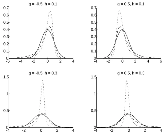
2.5.5 Properties of the G-and-H Distribution . . . 34

2.5.6 Subadditivity of VaR . . . 37

3 VaR and CVaR Optimization 41

3.1 CVaR Optimization . . . 41 3.1.1 Linearity of CVaR Optimization . . . 41 3.1.2 Reduction of Dimensionality using Benders

Decompo-sition . . . 42 3.2 VaR Optimization for Certain Classes of Asset Returns . . . . 45 3.2.1 Spherical and Elliptical Distributions . . . 45 3.2.2 Stable Distributions with Constant Skewness Parameter 48 3.2.3 Stable Distributions . . . 50

A Polynomial Algorithm for Stable Distributed Asset Returns . . . 50 Numerical Evaluations of Assumption AST _{. . . 52}

3.2.4 First Estimations for G-and-H distributed asset returns 57 3.3 Approximative Results for the VaR Optimum . . . 62

3.3.1 Using G-and-H Distributions to Match Real-World Op-timization Problems . . . 62 Numerical evaluations of the conditions for the

approx-imate approach . . . 65 3.3.2 VaR-optimization for general distributions . . . 73 Estimations for arbitrary distributions . . . 73 Error estimations using best linear and quadratic

4 Stochastic Branch & Bound 85

4.1 General Method . . . 85

4.1.1 The Algorithm . . . 86

4.2 Application to V aROptimization . . . 88

4.3 An Analysis of the Algorithm’s Efficiency . . . 94

5 Conclusion and Further Investigations 96

A Abbreviations and Notations 98

B Subadditivity of VaR for Stable Distributions 100

Danksagung

An dieser Stelle möchte ich Herrn Prof. Dr. Richert ganz herzlich für die Unterstützung bei meiner Dissertation danken. Ein weiterer Dank gilt allen Freunden und Kollegen bei der Münchener Rück, welche meine Arbeit durch anregende Diskussionen unterstützten. Derfinanziellen Unterstützung durch die Münchener Rück in Form eines Promotionsstipendiums sei eben-falls gedankt.

Die vorliegende Dissertation beschäftigt sich mit der Lösung einer sehr all-gemeinen Problemstellung, bei der für ngegebene Zufallsvariablen

X1, ..., Xn ∈R

die gewichtete ”Mischung”

X(x) :=x1·X1 +...+xn·Xn (0.1)

für x1, ..., xn ∈ R näher untersucht werden soll. Hierbei wird unterstellt,

dass die Abhängigkeitsstruktur der Zufallsvariablen X1, ..., Xn als bekannt

angenommen werden kann und als explizite Szenarienvektoren

Xi =

⎛ ⎜ ⎝

X1

i

.. .

Xk i

⎞ ⎟

⎠, X_ij _∈R

der Länge k vorliegen. In dieser Schreibweise ist die Abhängigkeitsstruktur durch die Ausprägungen von Xij für i = 1, ..., n implizit gegeben1. Weiter

sollen die Gewichte xi füri= 1, ..., nunter Einhaltung einer festgelegten

er-warteten Ausprägung_E(X(x))so gewählt werden, dassX(x) eine möglichst geringe Varianz aufweist.

Darüber hinaus wurde der Fall untersucht, bei welchem einseitige positive Abweichungen vom Erwartungswert keiner Beschränkung unterliegen, während das Unterschreiten eines vorgegebenen Schwellenwertes als Abweichung von der Erwartung mit möglichst hoher Konfidenz ausgeschlossen werden kann.

1 _{Durch die Verwendung einer geeigneten Anzahl an Szenarien k können über diesen}

Ansatz auch als stetig vorausgesetzte Zufallsvariable hinreichend approximiert werden.

vi

Mit anderen Worten soll die optimierte Mischung der Xi für zulässige Werte

xi bestimmt werden, so dass zu gegebener Konfidenz das Unterschreiten eines

Schwellenwertes durch die Zufallsvariable X(x) ausgeschlossen werden kann. Auch wenn der oben beschriebene allgemeine Fall an einem konkreten Beispiel erarbeitet wird, so ist hervorzuheben, dass an keiner Stelle der Analysen die Allgemeinheit der Aussage beschränkende Annahmen einfließen. Wird also das vorliegende Problem an einem konkreten Praxisbeispiel erläutert, so di-ent dies einzig und allein der Anschaulichkeit. Unbenommen hiervon handelt es sich bei dem vorgestellten Algorithmus um eine sehr allgemeine ”Quantils-Optimierung” einer beliebigen Mischung von Zufallsvariablen, wobei der Er-wartungswert der untersuchten Verteilung als bekannt vorausgesetzt wer-den darf. Bei dem beschriebenen Lösungsalgorithmus handelt es sich um eine Vorgehensweise, welche ohne weiteren Anpassungsbedarf auf allgemeine mathematisch-statistische Problemstellungen angewendet werden kann. Wie bereits erwähnt wurde, wird die oben beschriebene allgemeine Problem-stellung anhand einer konkreten ProblemProblem-stellung eingehend analysiert. In der Tat beschäftigen wir uns im vorliegenden Fall mit einer Erweiterung des klassischen Portfoliooptimierungsproblems, welches erstmals von Markowitz in seiner wegweisenden Arbeit [34] im Detail untersucht wurde. Die bere-its beschriebenen Zufallsvariablen Xi werden in diesem Zusammenhang als

Verlustverteilungen einzelner Assetklassen interpretiert und in der Markow-itzschen Analyse als normalverteilt unterstellt. Basierend auf dieser An-nahme wird das optimale Portfolio als eine Positionierung zwischen Risiko und erwartetem Verlust formuliert. Über den ursprünglich von Markowitz gewählten Ansatz hinaus wollen wir uns jedoch nicht auf den Fall normalverteil-ter Zufallsvariablen beschränken, sondern die Verlustverteilungen, gegeben als die Zufallsvariablen Xi, i = 1, ..., n mit größtmöglichem Freiheitsgrad

wählbar erlauben. Interpretieren wirx_∈Rn_{als Portfolioallokation dern}

ver-schiedenen Assetklassen, so ergibt sich die entsprechende Verlustverteilung

X(x) mittels Gleichung 0.1.

Eine sehr verbreitete Vorgehensweise zur Risikomessung bei nicht normalverteil-ten Verlustverteilungen stellt die Verwendung des Value-at-Risks zum Kon-fidenzniveau η (V aRη oder kurzV aR) dar. Dieses Risikomaß mißt den

kle-insten zu erwartenden Verlust, so dass die Wahrscheinlichkeit eines denV aR

klas-sifizierendes Risikomaß handelt, wird die Ausprägung der den V aR über-steigenden Verluste nicht berücksichtigt. In diesem Sinne wird bei gleicher Wahrscheinlichkeit des den V aR übersteigenden Verlusts die Situation, in welcher eine Konzentration von Verlusten den VaR deutlich übersteigt nicht unterschieden von einer (oftmals favorisierten) Verlustverteilung, bei welcher die Verluste geglättet über ein weites Spektrum unterschiedlicher Verlustaus-prägungen auftreten.

Es gibt eine Vielzahl an Bemühungen, Optimierungsprobleme der vorliegen-den Art effizient zu lösen. Ein Grund dafür, dass es noch immer keinen Algo-rithmus zur effizienten Lösung großdimensionierter Problemstellungen gibt, ist hauptsächlich in der fehlenden Subadditivitätseigenschaft des V aR be-gründet. Eine direkte Konsequenz ist im Allgemeinen das Auftreten zahlre-icher lokaler Optima, welche die Verwendung klassischer Lösungsansätze von vornherein ausschließen. In der Tat können Yang et al. in ([62]) zeigen, dass die Komplexität des Optimierungsproblems mit demV aR als Zielfunk-tion in die Klasse NP-schwieriger Problemstellungen fällt. Die Behauptung von Yang et al. wurde erneut aufgegriffen und in verallgemeinertem Kon-text mit neuer Beweisführung nachvollzogen. Aufgrund der Komplexität des Problems gibt es in der Forschung derzeit verschiedene Richtungen, um das Problem fehlender Subadditivität zu umgehen.

In einem ersten Schritt kann eine deutliche Reduktion der Komplexität durch die Beschränkung auf bestimmte Verlustverteilungen erzielt werden. Neben den bereits erwähnten, normalverteilten Verlustverteilungen zählen auch el-liptische Verteilungsannahmen zu jenen Verteilungen, für welche das kor-respondierende Allokationsproblem mittels geeigneter Algorithmen effizient gelöst werden kann. Darüber hinaus konnte in dieser Arbeit erstmals gezeigt werden, dass unter der Annahmeα-stabil verteilter Verluste und bestimmter (wenig restriktiver) Beschränkungen an das zu untersuchende Konfidenzniveau

η das ursprüngliche V aR Optimierungsproblem ebenfalls deutlich in seiner Komplexität reduziert werden kann.

vorliegen-viii

den Dissertation konnte dieses Resultat dazu verwendet werden, um unter wenig beschränkenden Annahmen an die Verlustverteilungen und für zahlre-iche Konfidenzniveausηstets ein affinesCV aR-Konfidenzniveau anzugeben, so dass die korrespondierende Lösung des CV aROptimierungsproblems eine oftmals ausreichende Approximation des ursprünglichen V aRProblems dar-stellt. Die Subadditivität der affinen Problemstellung erlaubt es mit Hilfe von Optimierungsverfahren zur Lösung hochdimensionaler linearer Problemstel-lungen auch das ursprüngliche Optimierungsproblem für eine äußerst große Anzahl an Freiheitsgraden xi effizient zu lösen. Eine Beschreibung aller

hi-erfür notwendigen Annahmen als auch Aussagen über die Güte der erzielten Approximation stellt den zentralen Bestandteil dieser Arbeit dar.

Sollen einerseits möglichst allgemeine Verlustverteilungen abgebildet werden und andererseits die Verwendung des V aRals Zielfunktion aufrecht erhalten bleiben, so existieren auch hier unterschiedliche Ansätze, welche im Allge-meinen allerdings nur für eine sehr begrenzte Zahl an zu optimierenden Frei-heitsgraden xi effiziente Anwendung finden. Eine hierunter fallende Klasse

Introduction

Within this thesis we want to address the solution of a very general problem setting, where for n given random variables

X1, ..., Xn ∈R

the weighted composition

X(x) :=x1·X1 +...+xn·Xn (1.1)

for x1, ..., xn ∈ R is analyzed in detail. Here, we presume the dependency

structure among the random variables X1, ..., Xn to be known and given as

scenario vectors of length k

Xi =

⎛ ⎜ ⎝

X1

i

.. .

Xik

⎞ ⎟

⎠, X_ij _∈R

Using this notation the dependency structure is given implicitly using real-izations of the X_ij, i = 1, ..., n1_{. Furthermore, the weights x}

i for i = 1, ..., n

are to be chosen in such a way that the expected value _E(X(x)) admits a preassigned value and such that X(x) admits the lowest variance possible.

1 _{Using an appropriate number of scenarios k, also continuous random variables can be}

approximated sufficiently.

2

Moreover, the case, where there are no bounds on the one-sided positive deviations from the mean, whereas the shortfall of a given threshold can be excluded with high confidence, is analyzed. In other words, the optimized composition of X(x) for feasible xi is to be determined in such a way that

for some given confidence the shortfall of a threshold can be excluded. While the general problem setting described above is worked out using a very special example, it is important to point out that at no point of the analy-sis the generality of the results restricting assumptions are made. When the problem at hand is explained using a concrete practical example the only rea-son for this is clearness. Besides this, the developed algorithm deals with the optimization of quantiles of a general weighted composition of random vari-ables under a predetermined value of its expected value _E(X(x)). Without any further efforts, the algorithm can therefore easily be applied to general mathematical and statistical problem settings.

As already mentioned above the more general problem setting at hand is analyzed using some concrete example. In fact, we want to address the classical portfolio optimization problem at first rigorously investigated by Markowitz’s pioneering work [34] on portfolio selection. There, Markowitz allows for the different asset classes’ returns to be normally distributed and based on this forecast he constructs the optimal portfolio as the right trade-off between risk and expected return. In our setting we will also act on the assumption that the underlying universe of asset classes has been predefined by well-known distribution functions. However, we will not restrict to the case of normal distributions but accept almost any kind of distributions as given by random variablesXi, i= 1, ..., n. Writingx∈Rn and interpreting it

as some portfolio allocation, the corresponding loss distribution of portfolio

x is then given by equation 1.1.

There have been many efforts of efficiently solving optimization problems where the V aR appears either in the objective function or is part of the constraints. The reason that there is still no solver at hand which can handle large scale problems is mainly due to the fact that theV aRrisk measure lacks subadditivity. A direct consequence is (in general) the existence of numerous local optima that exclude the usage of classical solvers such as the steepest descent method. In fact, Yang et al. show in ([62]) that the plain vanilla

V aR optimization as considered in this thesis is NP hard if accounting for general loss distributions. Due to this result there are now several different directions current research addresses the solution of this problem.

The first possible reduction in complexity can be achieved by restricting oneself to a special class of distribution functions. It is widely known that assuming normally distributed asset returns results in a V aR optimization problem that is equivalent to the problem of minimizing standard deviation. A similar structured problem is the wider class of elliptically distributed returns, not only since this class again inherits the property of being closed under taking the sum of elliptically distributed returns. Another class of distribution function which inherits this property is the class of α-stable distributed returns. We will show that under some minor assumptions on the confidence level the complexity of the corresponding V aR optimization problem will only be of polynomial type.

4

to this risk measure as CV aR, regardless of the distribution function being continuous or discrete. That this measure of risk is in fact a coherent one for an almost arbitrary choice of distribution functions was shown only recently by the authors Uryasev and Rockafellar ([52] and [53]). The mean absolute deviation ([30]), the mean regret ([13]) and the maximum deviation ([63]) are some further examples of risk measures which, dealt as the objective of the corresponding portfolio optimization problem, can be stated as a linear optimization problem. Moreover, Cheklov et al. ([9]) develop a risk measure called conditional drawdown-at-risk (CDaR) closely related to the concept of CV aR. The subadditivity property ofCDaRis also shown to hold true. Another possible approach in reducing complexity is the restriction to higher moments such as skewness and kurtosis besides mean value and standard deviation as in the Markowitz approach. This proceeding is based on the fact that the value at risk under some assumptions on the distribution function can be developed into a series of its central moments. This is done in an analogous way to the Taylor series expansion for differentiable functions and depends on different techniques such as the Cornish-Fisher or Gram-Charlie expansion ([25]). The author in [48] chooses a Cornish-Fisher expansion accounting for an additional skewness parameter in the objective function. However, this skewness parameter is set to be constant, hence it is not varying with the different portfolio allocations.

Investigation of the strong relationship between CV aR and V aR being the central topic of this thesis, it is worth to mention again the very promising approach of usingCV aRinstead of theV aRobjective in portfolio optimiza-tion. Whereas from a practitioner’ss point of view CV aR can be shown to be always the more conservative measure of risk Uryasev and Rockafellar succeed in proving the coherence of this measure thereby showing superior-ity when compared toV aR since it is exactly this property which allows for optimization problems to be easily solved. Dealing with a relatively easy to solve measure of risk on the other hand enables numerous other authors to solve for more advanced settings. For example Krokhmal et al. in [31] extend the setting to problems with CV aRbeing part of the constraints. Moreover, they investigate the efficient line within theCV aR framework.

We now want to give a short overview on the different meander towards our final result as stated in section 3.3. Before using g-and-h distributions to cope the matching of arbitrary distributions, we tried to investigate several other methods of approximation. First, as already mentioned before, we used different series such as Edgeworth-, Gram-Charlier- or Cornish-Fisher-Series which all approximate the respective probability functions in terms of their cumulants, hence can be used to approximately express both V aR

and CV aR. However, convergence of the corresponding series is not always guaranteed and the error of truncating the series after somefinite cumulant to our knowledge cannot be estimated within the portfolio context. Moreover, it is not entirely clear how to handle the additional cumulants in the portfolio optimization process.

Next we tried to use the approximate result for stable distributed returns already at hand to extend it to arbitrary distributions by approximating them through α-stable distributions. It is important to note, that using stable distributions to approximate the original V aR-problem directly, one has to find an appropriate function on the n-dimensional sphere, since such a function can be shown to give a dependence structure for multidimensional stable distributed random vectors (see e.g. [2], [42] or [39]). In order to significantly reduce complexity of the related optimization problem, we have to guarantee convexity of CV aRζ(x) as a function of portfolio composition

x. This can only be done by giving an overall dependence structure, as can be seen by following the proofs in [52]. However, the adaptation of a general dependence structure, as the search for an appropriate function on the n -sphere, to arbitrary distributions seemed too inflexible and too expensive. Our third approach was driven by the observation, that in general the V aR

mo-6

ments of a distribution. Again using the result for stable distributed asset returns, we tried to make usage of truncated stable distributions in order to firstly approximate the original distributions via thefirst three moments. In a second step we tried to use small truncation parametersλ >0(see e.g. [35] for the work with truncated distributions) of the truncated stable distribu-tion to best approximate a correspondingV aR/CV aR-optimization problem characterized by the parameter values (µ(x),σ(x),β(x)) which again corre-spond to the expected value, standard deviation and skewness, respectively. However, this proceeding also has several disadvantages. On the one hand, approximation by only the first three moments may not be enough to yield appropriate results. Moreover, to match the stable distribution by the corre-sponding truncated stable distribution would lead to the usage of very small values λ. This on the other hand leads to very small valuesσ(x),β(x) with problems for the corresponding optimization problem. Besides these disad-vantages, convexity of the resulting CV aR-optimization problem cannot be guaranteed.

We firstly develop the general notations used dealing with the V aR and

CV aR objective in Chapter 1. After introducing the main definitions and properties of these two risk measures we next have a closer look on the complexity of the general V aR optimization problem. Moreover, in this introductory chapter, Section 2.5 gives a rough overview on the two major families of distribution functions used in this thesis, stable distributions and g-and-h distributions.

Chapter 2 starts with solving theCV aRoptimization problem as transform-ing it to a linear programmtransform-ing problem. In a second step Benders decom-position is used to reduce the dimensionality of the resulting linear problem. Having recognized theCV aRoptimization problem to be of polynomial com-plexity, we analyse polynomialV aRoptimization problems for special classes of distribution functions in Section 3.2. In the subseeding sections we firstly use g-and-h distributions to match arbitrary distribution functions in order to find approximate statements for the euclidean distance between the V aR

optimum and the CV aR optimum for some suitably chosen confidence level

ζ0 ∈ (0,1). The necessary conditions for this estimation are considered

Chapter 2

Problem Statement and

Conjecture

2.1

General Notations and De

fi

nitions

Throughout this thesis, random variables are denoted by capital lettersY, Z, X, X1, ... and are assumed to be defined on a common probability space

(Ω,_F,_P). The distribution of the random variable Xi, i = 1, ..., n can be

interpreted as a loss distribution, giving the probability of losses for the respective insecure investments. Clearly, using this setting, _E(Xi) is to be

interpreted as the mean value of the loss distribution, hence the negative of the corresponding return distribution. We will denote by x = (x1, ..., xn)t ∈

Rn the concrete portfolio compositions given as the percentage allocations to the investment possibilities, i.e. xi denotes the percentage exposure to asset

class Xi, i = 1, ..., n. The set of permissible portfolio allocations is denoted

by _{X ⊂ R}n and is restricted to be a subspace of _Rn given, for example, in standard form

X=_{x_∈Rn _|Ax=b, x _≥0_} withA_∈Rm×n_{, b}

∈Rm_{. Moreover, we will always require to be fully invested}

without the possibility of going short, i.e. the minimum requirement on _X will be

X= x= (x1, ..., xn)∈Rn: n

i=1

xi = 1, xi ≥0, i= 1, ..., n . (2.1)

V aR andCV aR.

Definition 2.1.1 Forx_∈X,η _∈(0,1) theV aRη(x)is implicitly defined by

V aRη(x) := inf{z ∈R:P{X(x)≥z}≤η}. (2.2)

Moreover, for x _{∈ X},ζ _∈ (0,1), the expected shortfall CV aRζ(x) is defined

by

CV aRζ(x) := E[X(x)|X(x)> V aRζ(x)]. (2.3)

Remark 2.1.1 It is important to note that Definition 2.2 is suitable for con-tinuous distribution functions as well as for discrete ones. However, in the case of discrete distribution functions (as in any real world example charac-terized by scenario representations) more subtle definitions are required for rigorously defining expected shortfall, c.f. [53]. The same authors show that by dealing with the discrete case one can define CV aR as1

CV aRζ(x) := inf

a∈R a+

1

1₋ζE[X(x)−a]

+

, (2.4)

where[z]+= max(z,0).It is shown that for smooth distribution functions both definitions are equivalent (compare Theorem 10 in [53]). Since the expected shortfall is nothing else than a conditional expectation, the aforementioned definitions are not the only possible way of defining CV aR. If X(x) admits a probability density function fx(t), this can be used to define CV aR as

CV aRζ(x) =

1 1₋ζ

∞

V aRζ(x)

t_·fx(t)dt.

If the distribution function Fx under consideration is smooth, it is easy to

see that Definition 2.2 is equivalent to

V aRη(x) =Fx−1(α).

Remark 2.1.2 Comparing the two definitions for V aR and CV aR, it be-comes obvious that while V aRis not handling the extend of the losses beyond

2.1. GENERAL NOTATIONS AND DEFINITIONS 10

some threshold, taking the conditional mean in the definition of CV aR al-lows for the recognition of the loss structure beyond this threshold. Whilst only providing some lower bound for the losses in the tail, V aR is the more optimistic risk measure if compared to the more conservative usage ofCV aR. Compare the discussion in ([53], p. 1444).

Definition 2.1.2 During the whole paper, we will mainly focus on the fol-lowing two optimization problems

min

x∈XV aRη(x) (2.5)

and

min

x∈XCV aRζ(x). (2.6)

for various confidence levels η,ζ _∈ (0,1). However, in order to show some equivalence results of these two optimization problems we will also solve the problem

min

x∈XCV aRζ0,c(x), (2.7)

where we denote by

CV aRζ0,c(x) :=cσ(x)·CV aRζ0(x) +µ(x)

the CV aR objective with transformed scaling parameter cσ(x). CV aRζ0(x)

is thereby defined to be

CV aRζ₀(x) :=CV aRζ₀

x₋µ(x)

σ(x) .

Remark 2.1.3 Without explicitly referring to it, the usage of a transformed scaling parameter cσ(x) will always assume the existence of an appropriate scaling parameter σ(x).

As noted earlier, the set_Xcan also account for different linear restrictions to the optimization problem. In particular, restrictions on the minimum achiev-able return of the optimal portfolio allocation, denoted byx∗

η respectivelyx∗ζ,

Karush-Kuhn-Tucker conditions. To guarantee nondegeneratedness of these necessary conditions for a local minimum x∗_{, a number of regularity} condi-tions, such as the Linear Independence Constraint Qualification (LICQ) were developed (see e.g. [37]). The LICQ states that the optimization problem is regular inx∗_{if the gradients of the active inequality constraints and the} gra-dients of the equality constraints are linearly independent atx∗_{. Xas defined} in equation 2.1 clearly satisfies LICQ since at least one of the constraints is not active. The inclusion of additional constraints, however, must be in a way such that we are dealing with x∗ _{being regular.}

Besides the plain vanilla optimization problems as stated in (2.5) and (2.6) and its extensions to the generation of efficient lines, there exist various interesting generalizations that account for more complex settings. Among all these possible extensions we would like to emphasize the incorporation of liabilities in the present context rather than restricting oneself to the analysis of an asset only portfolio. The optimal matching of stochastic liabilities that cannot be directly influenced by changing some portfolio allocation is known as Asset Liability Management (ALM) and attains increased significance not only in the insurance industry but also within corporate companies and investment banks. Considering stochastic liabilities as an additional input parameter to the optimization problem can have a tremendous effect on the optimal allocation x∗_{. Denoting by ξ some arbitrarily distributed random} variable, those liabilities ξ could easily be incorporated by setting

X :=X(x) := (X1, ..., Xn)·

⎛ ⎜ ⎝

x1

.. .

xn

⎞ ⎟

⎠+ξ,

2.2. FORMULATION OF THE ALGORITHM 12

2.2

Formulation of the Algorithm

To describe the fundamental algorithm of this thesis, we will firstly have to introduce a set of striking portfolio compositions. Based on the optimization problem (2.7) we therefore define

X∗ := x_∈X|xsolution of (2.7), ζ _∈(0,1), c_∈R+ .

and denote by x∗

ζ,c the respective elements of X∗. Furthermore, by x∗ζ we

will shorthand refer to the portfoliox∗_ζ,1.We will then consider the following optimization problem

min

x∈X∗V aRη(x) (2.8)

and show that the resulting optimal portfolio is either equal to the solution of the original problem (2.5) in the case of specially distributed asset returns. For those cases, where we are not able to show exact matching of optimal portfolios, we will state an upper bound for the euclidean distance of the two portfolio compositions as given by the arguments of (2.5) and (2.8). Hence, in searching for the global minimum of the original (maybe huge dimensional) problem one gets reasonable results in restricting oneself to the set _X∗ _and therefore reducing to a two dimensional search which generally is much more efficient to solve. Moreover, some of the results of this thesis choosecin the definition of the set_X∗_{to be equal to one hence resulting in a one dimensional} search equivalent. It is interesting to note, that in those cases, where we allow for an arbitrary positive valuec, we found that the optimal value forcin the sense of (2.8) is also close to one.

Therefore, the main complexity in order to solve (2.8) lies in the determina-tion of the set_X∗ which itself heavily depends on the effective solution of the affine CV aR optimization problem for suitable confidence levels ζ _∈ (0,1).

There we can use Rockafellar’s and Uryasev’s result on efficiently optimizing

CV aRfor somefixed confidence levelζ.In practice, for a suitable choicecl,cu

we will take some sufficiently close meshed grid on(0,1)_×[cl, cu]and for every

element (ζ, c) on this grid we solve the corresponding CV aR optimization problem. That this procedure in fact will produce a helpful approximation to the set _X∗ _{is the result of the next lemma which states that optimization} (2.8) generally is well behaved.

Lemma 2.2.1 Let V aRη(x) be a continuous function of x and suppose that

CV aR optimization problem (2.6). Then for c >0 the function

h: (0,1)_−→R (2.9)

ζ _−→V aRη x∗ζ,c

is continuous.

Proof: W.l.o.g. we can restrict to the case c = 1. Other values of c do not change the qualitative statement. We prove continuity in an arbitrarily chosen confidence levelζ0 ∈(0,1).

Step 1: CV aRζ(x) is a continuous function of the confidence level ζ. This

result was proven for arbitrary distribution functions in ([53]). Step 2: The mapping

ζ _−→CV aRζ(x∗ζ)

is continuous. For each a_{∈ R} consider the function of γ _∈R, x_{∈ X} defined by

θa,x(γ) =a+γE (X(x)−a)+ ,

and let

θ(γ) = min

x∈X,a∈Rθa,x(γ). (2.10)

Hence by Theorem 10 and 14 of ([53])

CV aRζ(x∗ζ) ≡ min

x∈XCV aRζ(x)

= min

x∈X,a∈Rθa,x(γ)

= θ(γ) for γ = 1/(1₋ζ), (2.11)

with the minimum in (2.10) being attained when a belongs to the interval [V aRζ(x∗ζ), V aR

+

ζ(x∗ζ)].

According to (2.10),θ is the pointwise minimum of the collection of functions

θa,x. Those functions are affine, hence θ is concave (c.f. [51], Theorem

5.5). A finite, concave function on _Rn _{is necessarily continuous (c.f. [51],}

2.3. COMPLEXITY OF THE VAR-OPTIMIZATION PROBLEM 14

ζ _→ CV aRζ(x∗ζ) as the composition of θ with ζ → 1/(1−ζ) and invoking

the chain rule.

Step 3: The mapping

ζ _−→x∗_ζ (2.12)

is continuous. Using continuity of Step 1, for anyε>0there exists aδ1 >0,

s.t.

|ζ₋ζ_0|<δ1 ⇒ CV aRζ(x∗ζ0)−CV aRζ0(x

∗

ζ0) <

ε

2 Moreover, by Step 2 there exists δ2 >0, s.t.

|ζ₋ζ0|<δ2 ⇒ CV aRζ(x∗ζ)−CV aRζ0(x

∗

ζ0) <

ε

2

Defining δ:= min_{δ1,δ2}and for all confidence levels ζ satisfying|ζ−ζ0|<

δ we can write

CV aRζ(x∗ζ)−CV aRζ(x∗ζ0) ≤ CV aRζ(x

∗

ζ)−CV aRζ0(x

∗

ζ0)

+ CV aRζ0(x

∗

ζ0)−CV aRζ(x

∗

ζ0)

< ε

2 +

ε

2 =ε

Hence by the convexity ofCV aRand the assumed uniqueness of its optimum for any sufficiently smallδ >0, ε>0can be chosen, s.t.

x∗ζ−x∗ζ₀ <δ.

Since V aRη(x) is a continuous function of the portfolio composition x, also

the composition with the continuous function as defined in (2.12) is

contin-uous which is the claim of the lemma.

2.3

Complexity of the VaR-Optimization

Prob-lem

The authors in [62] investigate the optimization problem 2.5 and show that the problem offinding the optimal allocationx∗

ηis generally Non-deterministic

Although being formally correct, in their proof to NP-hardness, the authors are using some predefined distribution function of the individual asset classes. Moreover, the number of used scenarios is not to be arbitrarily chosen and the proof only allows for the confidence levelη = 1₂. Hence, it is not entirely clear if the optimization problem looses its property of being NP-hard when we are allowing for an arbitrary number of scenarios and/or if we are only interested in some confidence level close to one. Below, we are stating an alternative (and in our sense more intuitive) proof of NP-hardness, thereby accounting for the above mentioned remedies.

Theorem 2.3.1 The scenario-basedV aRη optimization problem (2.5) is

NP-hard.

Proof: Suppose there exists some joint continuous density functionp(y)for the losses denoted byy. Before reducing the NP-hard ”Subset Sum” problem to the current one, let us implicitly define V aRη using the joint density

function

x·y≥V aRη

p(y)dy =η.

The main complexity in solving for the optimal portfolio allocation in (2.5) lies in the decision whether or not there exists a feasible solution which accounts for some predefined value V aRη (c.f. [62]). To be more rigorous,

denoting by V the minimum achievable value of the original problem,

V := min

x∈XV aRη(x),

for some given value Vt_{, problem (2.5) is in complexity equivalent to the}

decision whether there exists x_∈X with

x·y≥Vt

p(y)dy =η. (2.13)

Discretising Equation 2.13 yields2

min

⎧ ⎨ ⎩_x·y

i≥Vt

p(yi)| x·yi≥Vt

p(yi)≥η

⎫ ⎬

⎭ (2.14)

2.3. COMPLEXITY OF THE VAR-OPTIMIZATION PROBLEM 16

for loss values yi. Suppose now there exists a polynomial algorithm that

decides for any joint density function and any choice of loss values yi, i =

1, ..., nwhether there exists a correspondingx_∈X, s.t. (2.14) holds. Defining

ai

kak :=p(yi)∀i= 1, ..., nand

S1 : = ai |xyi ≥Vt

S2 : = ai |xyi < Vt

the problem is equivalent to the one of deciding whether there exists a subset

S1 of S :={a1, ..., an}, s.t.

ai∈S1

ai =η. (2.15)

which by assumption would also be solvable within polynomial time. This would be in contradiction to the well known fact that the so called Subset Sum problem (2.15) is NP-hard (compare [56]). Note that the existence of a joint density does not generally imply the cor-responding V aR problem to be hard to solve. For example, the case of normally distributed asset returns with joint distribution function is known to be easily treatable. Moreover, J. Danielsson et al. (c.f. [11]) give some further examples where either the confidence level or the special structure of the distribution functions are chosen in a way that the resulting optimization problem is of polynomial type. All these examples correspond to some simple structured Subset Sum problem as in the proof of the theorem. However, fol-lowing the lines of the theorem, one attains any kind of Subset Sum problem by a suitable choice of the joint density function.

Although we cannot give a rigorous proof, the experience of the calculations to this thesis as well as the results given below teaches most of the undesired behavior to be caused by discretising the originally assumed continuous or even differentiable distribution functions. Discretising the random variables to work with numerically seems to produce a large number of local extremas that would not be observed solving the problem analytically. Using the advantage of convexCV aRoptimization in the proposed algorithm forV aR

2.4

Properties of VaR and CVaR

Within this section we want to present the major properties of the two risk measures under consideration. It is not our intention to give a full review of all the V aR and CV aR inherent properties but to restrict to those proper-ties that are directly used in our approach of minimizingV aR. In particular, we will concentrate on the coherence of V aR and CV aR as well as stating some important relations between those two risk measures. The subaddi-tivity property will be seen to be the crucial difference between the two risk measures; its absence is the reason for the increased complexity in optimizing

V aR.

2.4.1

Coherent Measures of Risk

Artzner et al. [4] show that there exists a set of axioms that risk measures should fulfill. The authors also show that these axioms are complete in the sense that if a measure does not satisfy all the axioms, this may lead to undesirable conclusions. Considering a setV of real valued random variables withρ describing some arbitrary risk measure, these axioms can be stated as

(a) (translation invariance) Y _∈V, c_∈R⇒ρ(Y +c) =ρ(Y) +c

(b) (positive homogeneity) Y _∈V, c >0, cY _∈V _⇒ρ(cY) =cρ(Y) (c) (sub-additivity) Y1, Y2, Y1+Y2 ∈V ⇒ρ(Y1+Y2)≤ρ(Y1) +ρ(Y2)

(d) (monotonicity) Y1, Y2 ∈V, Y1 ≺Y2 ⇒ρ(Y1)≤ρ(Y2)

where in (d) we used the relation Y1 ≺ Y2 iff E[ψ(Y1)] ≤ E[ψ(Y2)] for all

integrable monotonic functions ψ.

Without any further assumptions it can easily be seen (compare e.g. [47]) that both V aR and CV aR as defined above satisfy translation invariance, positive homogeneity as well as monotonicity. The property of being sub-additive is always fulfilled using ρ= CV aR, hence by positive homogeneity

CV aR admits the property of being convex in the sense that for 0<λ <1

2.4. PROPERTIES OF VAR AND CVAR 18

We will have a closer look at this property in Subsection 2.4.3. SinceV aRis not always subadditive (i.e. the property depends strongly on the confidence level and the setV used) it does not inherit convexity in general. Apart from the above described fact that V aR tends to be a too optimistic measure of risk, the lack of being subadditive is one of the major drawbacks of usingV aR

in risk management. Beyond accounting for nice mathematical properties, in practice the usage of convex risk measures has the advantage that risk measurement on a subsidiary level guarantees the overall risk not to exceed the sum of the individual risks. Using V aR this conclusion might be false and result in a wrong risk allocation. We will have a closer look on this topic in Subsection 2.5.6.

2.4.2

Relations between VaR and CVaR

V aR is a quantile whereasCV aR measures the conditional tail expectation. Hence these two risk measures obviously coincide only if the tail is cut off and the cut is in V aRη(x) itself. Nevertheless, within the next theorem we

will state two very important relations between V aR and CV aR.

Theorem 2.4.1 (i) Considering the same confidence level ζ for V aR and

CV aR, CV aRζ(Y) always succeeds V aRζ(Y),

V aRζ(Y)≤CV aRζ(Y),

for any random variable Y.

(ii) WritingFx for the distribution function of some random variable suppose

ζ is in the range of F, i.e. F(F−1_{(α)) =α, then}

CV aRζ(Y) =

1 1₋ζ

1

ζ

V aRε(Y)dε. (2.16)

b be chosen such thatF(b) =ζ. Then_P{Y > b_}= 1₋ζ and

E(Y _|Y > b) = E YI{Y >b} P{Y > b_}

= E bI{Y >b}+ [Y −b]

+

P{Y > b_}

= b+ 1

1₋ζE [Y −b]

+

.

This shows, that under the assumptions of the theorem equation (2.16) holds also when using the alternative definition of CV aR for discrete distribution

functions.

2.4.3

Subadditivity of CVaR

The main purpose of this paper is to solve theV aRoptimization problem by a sequence of affineCV aRoptimization problems. It is therefore not surprising that the aspect of efficientlyfinding the solution of theCV aRobjective is one of our main focuses. Since in practice we are always confronted with a finite set of scenarios representing some (theoretical) distribution function, we want to show that the above mentioned subadditivity property is not only true for sufficiently smooth distribution functions, but also holds for those cases where the distribution function is a discrete step function. In financial applications this is the only case of interest since any optimization has to be performed on a finite set of scenarios. Moreover, it is the intention of this subsection to formulate the corresponding CV aR optimization problem in a way that allows for a simple implementation. Hence this subsection can be interpreted to provide the necessary background for further developments of efficient

CV aR solvers as described in Section 3.1. All the results of this section can be found in the joint work of Rockafellar and Uryasev ([53]). Although the authors are dealing in a more general context, we are concentrating on the pure portfolio allocation problem hence stating their results in a more specialized framework.

As the authors in [53] show, using discrete distribution functions instead of continuous ones makes it necessary to distinguish between the definition of

V aRη(x) as given in (2.2) and

2.4. PROPERTIES OF VAR AND CVAR 20

However, this distinction only becomes relevant for a small number of sce-narios. If we are dealing with thousands of scenarios, the difference between the definition of V aR+

η(x) and V aRη(x) will only be marginal. For a small

number of scenarios an appropriate definition of analogous valuesCV aR+_ζ(x) and CV aR−_ζ(x) to the existing definition of CV aRζ(x) becomes necessary.

Since in this paper we are assuming to deal with a sufficiently large number of scenarios and since we do not need this distinction in the further course of this thesis, we will omit the corresponding definitions. For further details consult the above mentioned paper by Rockafellar and Uryasev.

We are now in the position to state one of the main advantages of using

CV aR overV aR as a risk measure.

Theorem 2.4.2 Considering the definition of CV aRζ(x) as given in 2.4

define

Gζ(x, a) :=a+

1

1₋ζE[X(x)−a]

+

,

with [t]+:= max_{0, t_}.

(i) Since X(x) is a linear function of x, Gζ(x, a) is a jointly convex

func-tion in x and a. In particular, CV aRζ(x) is a convex function of the

portfolio composition x.

(ii) Minimizing CV aRζ(x) as a function of x∈X is equivalent to

minimiz-ing Gζ(x, a) over all (x, a)∈X×R in the sense that

min

x∈XCV aRζ(x) =(x,amin)∈X×RGζ(x, a).

Moreover,

(x∗,ζ∗)_∈arg min

(x,a)∈X×RGζ(x, a)⇐⇒

x∗ _{∈arg min}

x∈XCV aRζ(x),

ζ∗ _∈arg mina∈RGζ(x∗, a)

Proof: For a full proof of the statements of the theorem see ([53]). The statement of the theorem can now be used to implement the correspond-ing CV aRζ(x) optimization problem in an efficient way. In fact, we will see

minimization problem as a linear one. Further simplifications using Benders decomposition can be applied in order to increase efficiency. We will focus on these developments in Section 3.1 below.

After having stated the subadditivity property of CV aRζ(x), we want to

show that this property is stable under some minor change of the objective. Below, we will show that the V aRη optimization problem is in some sense

and under several assumptions on the distribution functions equivalent to the detection of the CV aRζ0,c minimizing portfolio for some given (ζ0, c) ∈

(0,1)_×R+_{. Here, the objective function is given by}

CV aRζ0,c(x) :=c·σ(x)CV aRζ0(x) +µ(x),

again using CV aR to denote theCV aRof the standardized distribution. The next lemma shows that this objective function is also a convex function of the portfolio composition x_∈X.

Lemma 2.4.3 For all c _{∈ R}+_{, ζ}

0 ∈ (0,1) and under the assumptions of

Theorem 2.4.2 CV aRζ0,c(x) is a convex function of x.

Proof: Theorem 2.4.2 gives us the convexity of CV aRζ0,1(x). Hence,

c_·CV aRζ₀,1(x) is a convex function and we can write

c_·CV aRζ0,1(x) = c·σ(x)CV aRζ0(x) +c·µ(x)

= :CV aRaζ0,c(x),

Here CV aRaζ0,c(x) denotes the expected shortfall, where for all i = 1, ..., n

the original asset classes Xi are replaced by linearly transformed Xi with

µ(Xi) =cµ(Xi).It is important to note, that by the linearity of the expected

value µ(x), CV aRaζ0,c(x)is convex iffCV aRζ0,c(x) is convex.

2.4.4

Di

ff

erentiability of VaR and CVaR

Our results on the equivalence of the V aRη and the CV aRζ optimization

2.4. PROPERTIES OF VAR AND CVAR 22

composition x. First developments into this direction can be found in [24] and [23]. Although these papers already provide readily interpretable for-mulae for the case of linear combinations of random variables, the authors did not yet attend the question under whichsoever general conditions their formulae in fact hold true, hence addressing the question of differentiability. Addressing both the V aRand theCV aRrisk measure, Tasche in ([59], Sec. 5.2 and 5.3), develops some certain conditions under which differentiability is fulfilled. There one alsofinds some helpful discussion on distribution func-tions more frequently used in financial applications. For completeness, we will state those conditions summarized in Assumption (S). Compare ([59], p. 16) for the original context.

Assumption (S) For fixed η _∈ (0,1), we say that an _Rn _{valued random}

vector(X1, ..., Xn)satisfies Assumption (S) ifn≥2and the conditional

distribution of X1 given (X2, ..., Xn) has a density

Φ:_R×Rn−1 _−→[0,_∞) (t, x2, ..., xn)−→Φ(t, y2, ..., yn)

which satisfies the following four conditions

(i) For fixedy2, ..., yn the function t−→Φ(t, y2, ..., yn) is continuous int.

(ii) The mapping

R×R\{0_{} ×R}n−1 _−→[0,_∞)

(t, x)_−→E Φ x−11 t−

n

j=2

xjXj , X2, ..., Xn

is finite-valued and continuous. (iii) For each x_∈R\{0_{} ×R}n−1

0<_E Φ x−₁1 V aRη(x)−

n

j=2

xjXj , X2, ..., Xn .

(iv) For each i= 2, ..., d the mapping

R×R\{0_{} ×R}n−1 _−→R

(t, x)_−→E XiΦ x−11 t−

n

j=2

xjXj , X2, ..., Xn

Under these assumptions, Tasche shows thatV aRη(x)is a differentiable

func-tion of x. If the mean value of X(x) is finite, he also shows differentiability of CV aRζ(x). Moreover, he again develops the formulae first published in

[24] and [23] expressing the partial derivatives of V aRη(x)andCV aRζ(x) in

the following descriptive way

∂ ∂xi

V aRη(x) =E{Xi :X(x) =V aRη(x)}, i= 1, ..., n. (2.17)

similarly, the partial derivative of CV aRζ(x) yields the expressive form

∂ ∂xi

CV aRζ(x) =E{Xi :X(x)≥V aRζ(x)}, i= 1, ..., n. (2.18)

Scaillet in [55] derives similar formulas and discusses its application to the normal distributed case. Formulas (2.17) and (2.18) show the main difference between the two risk measures. Whereas under some assumptions on the dis-tribution function V aR appears to be partially differentiable, its derivative becomes in some sense unstable, indicating that generally only very restric-tive assumptions on the distribution function will yield derivarestric-tives of higher order. The aforementioned condition of being unstable becomes apparent when numerically evaluating expression (2.17). Having vectors Xi

represent-ing the random variable Xi, i= 1, ..., n, the corresponding partial derivative

can be approximated by taking the entry of Xi which corresponds to the

entry of Xt

·x which again representsV aRη(x).Obviously, such evaluations

can result in very different partial derivatives.

On the other hand, formula (2.18) can be used in a similar way byfirst sort-ing the vector Xi with respect to the sorted entries of Xt·x and taking the

mean over the (1₋ζ)_·100% of the last entries. Taking the mean makes the partial derivative much more stable. Expressions for the V aR and the

CV aR derivatives of arbitrary order are given in [50]. However, actual dif-ferentiability conditions for higher order derivatives in an arbitrary context are (to our best knowledge) not yet developed.

At some stage we are not only interested in the differentiability with respect to the portfolio composition but also in the differentiability with respect to the confidence level η. For distributions with continuous distribution func-tion, the result for V aR immediately follows from

∂

∂ηV aRη(x) = ∂ ∂ηF

−1

2.5. SOME COMMENTS ON STABLE / G-AND-H

DISTRIBUTED ASSET RETURNS 24

and the differentiability of the inverse function. Relation (2.16) gives the equivalent result for CV aR. For more general distribution functions the result might not hold true for the V aRrisk measure. UsingCV aRas a risk measure, Rockafellar and Uryasev show ([53], p. 1458) that even for discrete distributionsCV aRζ(x)is a continuous function ofζ which exhibits left and

right derivatives.

2.5

Some Comments on Stable / G-and-H

Distributed Asset Returns

Some of our results are heavily dependant on the usage of stable respec-tively g-and-h distributions. Whereas stable distributions admit the favor-able property of being closed under taking the sum, hence allowing for explicit representations in terms of the defining parameters, g-and-h distributions ex-hibit tremendous flexibility in matching arbitrary distributions. Moreover, theV aR for g-and-h distributed asset returns appears to be given by an ex-plicit formula. Because of the importance to our results, we will give a short overview on the properties of these two classes of distribution functions.

2.5.1

Properties of Stable Distributed Asset Returns

Within this paragraph we want to consider the class of stable probability distributions which can be interpreted as a generalization of the normal law allowing for skewness and heavy tails. This class was originally introduced by Paul Levy in the 1920s in his study of sums of i.i.d. terms. Since there is empirical evidence for skewness and/or kurtosis withinfinance and economic modelling this class of distributions is nowadays often used in the modelling of financial data. For a list of research on this topic we refer to the citations in [41]. Another reason for the usage of stable distributions is the Generalized Central Limit Theorem which states that the only possible non-trivial limit of normalized sums of i.i.d. distributed terms is again stable. Since it is argued that e.g. the price of stocks is the sum of many small terms consequently a stable model should be used to model this data.

a reason for the widespread distribution of this special kind of distribution function is justified by the development of reliable and fast methods to com-pute stable densities, distribution functions and quantiles. Moreover, as we will see in the next paragraph there were developed fast methods to generate stable random variables.

The class of stable probability distributions encloses some very nice theo-retical properties. However it is not our intention to give a full reference to all these properties. We will therefore restrict ourselves to those selected properties that are directly related to portfolio allocation and to our desire to find the optimal solution of the V aR optimization problem.

Every stable distributed random variable is uniquely defined by four para-meters: an index of stability or characteristic exponentα_∈(0,2],a skewness parameter β _∈ [₋1,1], a scale parameter γ > 0 and a location parameter

δ _∈R. Although there are several different representations used to describe stable distributions we are concentrating on the two most common ones. Moreover, within this thesis we will focus on the 1-parametrization (as in the notation of Nolan in [41]) for the reason that using this representation the location parameter δ corresponds to the mean value (forα>1). In order to implement efficientV aRandCV aRcalculators we mainly use the representa-tions of the distribution function as given in [38] where the 0-parametrization is used. To compare the results with the 1-parametrization we will have to adjust the values for δ accordingly. The respective transformation functions are given below.

Definition 2.5.1 For 0 < α _≤ 2, ₋1 _≤ β _≤ 1, γ > 0 and δ _{∈ R} a stable random variable X in the 0-parametrization, X _∈ Sα(β,γ,δ; 0), is given by

the characteristic function

Eexp(iuX) =

exp ₋γα

|u_|α 1 +iβ tanπα₂ (sign u) _|γu_|1−α₋1 +iδu if α= 1

exp ₋γ_|u_| 1 +iβ_π2 (signu) log (γ_|u_|) +iδu if α= 1.

2.5. SOME COMMENTS ON STABLE / G-AND-H

DISTRIBUTED ASSET RETURNS 26

some Cauchy distribution whereas the choice α = 1₂ represents Levy stable distributions.

We often handle standardized distributions, i.e. γ = 1 and δ = 0. In this case we will use Sα(β; 0) as an abbreviation of Sα(β,1,0; 0). Further on we

will also use the notation

V aRη(β(x))

to describe theV aRof a standardized random variableX 9Sα(β; 0).Similar

notations are used forCV aRas well as for the 1-parametrization as described next.

Definition 2.5.2 For 0 < α _≤ 2, ₋1 _≤ β _≤ 1, γ > 0 and δ _{∈ R} a stable random variable X in the 1-parametrization, X _∈ Sα(β,γ,δ; 1), is given by

the characteristic function

Eexp(iuX) = exp −γ

α

|u_|α 1₋iβ tanπα₂ (sign u) +iδu if α = 1 exp ₋γ_|u_| 1 +iβ2

π(sign u) log (|u|) +iδu if α = 1.

If not explicitly mentioned the 1-parametrization will be used denoted by

Sα(β,γ,δ) and Sα(β) for arbitrary and standardized stable distributions,

respectively. Within the two parametrizations described above,α,β and the scaleγ are always the same; the location parameter however admits different values for the same stable distributed random variable X 9 Sα(β,γ,δk;k)

for k = 0,1. Writing δ0 andδ1 for the location parameter of the respective

parametrization, one easily sees that

δ0 = δ1+βγtan

πα

2 ,for α= 1

δ1+β2_πγlogγ, forα = 1

δ1 = δ0−βγtan

πα

2 , for α= 1

δ0−β_π2γlogγ,for α= 1.

Therefore it is quite easy to transform between the two parametrizations. One of the most important properties of stable distributed returns is the fact that any linear combination of α-stable distributed r.v. is again α-stable distributed. Hence for some arbitrary portfolio composition x _{∈ X}, the resulting distribution function can be exactly described and analyzed by the behavior of the four parameters. The next theorem gives us somefirst insight to the behavior of these parameters as functions of the portfolio composition

Theorem 2.5.1 Let Xi 9Sα(βi,γi,δi;k), k= 0,1, be independently

distrib-uted random variables and let x = (x1, ..., xn)t ∈ X describe some feasible

allocation. Then

X :=x1·X1+...+xn·Xn9Sα(β(x),γ(x),δ(x);k).

Moreover, the parameters β,γ and δ are explicitly given by

γ(x)α =

n

i=1

|xiγi|

α

β(x) =

n

i=1βi(signxi)|xiγi|

α

γα (2.19)

δ(x) =

ixiδi+ tan

πα

2 (βγ− iβixiγi) if k = 0, α= 1 ixiδi+_π2 (βγlogγ− iβixiγilog|xiγi|) if k = 0, α= 1

ixiδi if k = 1, α= 1

ixiδi−

2

π iβixiγilog|xi| if k = 1, α= 1.

Proof: For a proof of this result we refer the interested reader to [54], [41].

In order to introduce some dependence structure among the different asset allocations it is practical to consider multivariate stable distributions. If we denote by

S:=_{u_∈Rn: u = 1_}⊂Rn

the unit sphere in_Rn,then Feldheim (in [19]) showed that any stable random vector can be characterized by a spectral measure Λ (a finite measure on _S) and a shift vector δ _{∈ R}n_{. Any stable random vector X} 9 _S

α(Λ,δ) can

therefore be represented as Eexp(i u,X )=

⎧ ⎪ ⎪ ⎨ ⎪ ⎪ ⎩

exp − S | u, s |

α

−i(sign u, s ) tanπα_{2 |} u, s _|α _·

Λ(ds) +i u,δ if α= 1

exp − S | u, s |

α

−i(sign u, s ) tanπα_{2 |} u, s _|α _·

Λ(ds) +i u,δ if α= 1

2.5. SOME COMMENTS ON STABLE / G-AND-H

DISTRIBUTED ASSET RETURNS 28

α-stable with some skewness β(x), some scale γ(x) and some shift δ(x).We will write X 9Sα(β(.),γ(.),δ(.)) if X is stable with

x,X 9Sα(β(x),γ(x),δ(x))

for every x _{∈ R}n _{(again implicitly using the 1-parametrization). Note that}

the spectral measure determines the projection parameter functions by

γα(x) =

S

| x, s _|αΛ(ds)

β(x) = S| x, s |

α

sign( x, s )Λ(ds)

γ(x)α (2.20)

δ(x) = x,δ α = 1

x,δ _{− π}2 _S x, s log_| x, s _|Λ(ds) α = 1

There exists no explicit formula for the density function nor the cumulative distribution function of anα-stable random vector. However, it can be shown that any nondegenerate (i.e. γ = 0) stable distribution is a continuous dis-tribution with an infinitely differentiable density function (compare [41]). In the univariate as well as in the multivariate case the authors Abdul-Hamid and Nolan ([1]) give integral representations of the density functions.

In the further proceeding we will implicitly use the differentiability of V aR

and CV aR as a function of the portfolio allocation. That this is indeed well-defined for stable distributions is the content of the next remark.

Remark 2.5.2 Suppose (X1, ..., Xn)t is a stable distributed random vector.

Then, by [1] there exists a multidimensional continuous density function

p:_Rn _→[0,_∞[.

In particular, p is a bounded function, such that for fixed x2, ..., xnthe

func-tion

p: _R→[0,_∞[

t_−→p(t, x1, ..., xn)

is continuous and for every u_∈R\{0_{} ×R}n−1

E p u−₁1_· V aRη(u)−

n

i=2

Moreover, by restricting oneself to α-stable random vectors with α >1, it is well known, that for i= 1, ..., n

E[_|Xi|]<∞.

Hence, Assumption S is satisfied for α -stable random vectors (α > 1) (cf. [59], p.17 following the discussion on special situation where Assumption S is satisfied) and thus (cf. chapter 2.4.4) V aRη(x) and CV aRζ(x) are partially

differentiable functions of x.

2.5.2

Generation of Stable Distributed Random

Vari-ables

If we want to investigate either the V aR or the CV aR structure of stable distributed portfolio allocations it is often helpful to generateα-stable distrib-uted random variables. By generating a large set of corresponding scenarios it is then relatively easy to get a rough idea of the V aR respectively the

CV aR behavior for different allocations. Although it does not seem obvious how to generate stable distributed random variables, Chambers et al. give an easy way of generating those r.v. based on a nonlinear transformation of two independent uniform respectively exponential distributed random variables.

Theorem 2.5.2 Let Θ and W be independent with Θ uniformly distributed on(₋π₂,π₂)andW exponentially distributed with_E(W) =1and let0<α _≤2.

(a) The symmetric random variable

Z = (cos)sinα1Θ/α

cos(α−1)Θ W

(1−α)/α

α= 1

tanΘ α= 1

(2.21)

has a Sα(0; 0) =Sα(0; 1) distribution.

(b) In the nonsymmetric case, for any ₋1_≤β _≤1, define

Θ0 = arctan βtan

πα

2 /α

when α= 1. Then

Z =

⎧ ⎨ ⎩

sinα(Θ0+Θ)

(cosαΘ0cosΘ)1/α

cos(αΘ0+(1−α)Θ)

W

(1−α)/α

α = 1

2

π π

2 +βΘ tanΘ−βlog

π 2WcosΘ

π

2+βΘ α = 1

2.5. SOME COMMENTS ON STABLE / G-AND-H

DISTRIBUTED ASSET RETURNS 30

has a Sα(β; 1) distribution.

Proof: A proof of this result can be found in [8]. To simulate stable random variables X with arbitrary scale and location parameters γ,δ one has to apply the following transformations

X = γ Z−βtan

πα

2 +δ α= 1

γZ+δ α = 1 (2.23)

in the 0-parametrization, whereas in the 1-parametrization the necessary transformations look like

X = γZ +δ α= 1

γZ + δ+β_π2γlogγ α= 1. (2.24)

2.5.3

VaR Computation in the

α

-stable Case

In principle, to perform theV aRcalculation for an arbitrary confidence level, it is possible to use equations (2.21), (2.22) to generate a set of random vari-ables, sort the corresponding vector and take the entry that corresponds to the α-quantile. However, if we are dealing with very heavy tailed distribu-tions as in the case of α near 1, especially for higher confidence levels the number of scenarios generated to yield an accurate value for the V aR esti-mate will have to be very high. To compass these difficulties with modeling the heavy tail directly, the so called technique of Importance Sampling was developed (see [57], [7]). However, in our context it will be a more efficient approach to calculate the corresponding distribution function and use this to determine the V aR. Nolan in [38] gives formulas for the density and distri-bution function of stable random variables that only involve the numerical evaluation of one integral over a finite interval. Since in the present context we are only interested in the formulas for the distribution function, we will not state the corresponding formulas for the density functions. For a numeri-cal implementation one should take into account the discussion on numerinumeri-cal considerations in [38], page 766.

Before we can state the exact formulas we will have to introduce some further notations. Define

ζ = ζ(α,β) = −βtan

πα

2 α= 1

0 α= 1

θ0 = θ0(α,β) = 1

αarctan βtan

πα

2 α= 1

π

2 α= 1

c1(α,β) =

⎧ ⎨ ⎩ 1 π π

2 −θ0 α <1

0 α = 1

1 α >1

V (θ;α,β) =

⎧ ⎨ ⎩

(cosαθ0)

1

α−1 cosθ

sinα(θ0+θ)

α

α−1 _{cos(αθ0+(α−1)θ)}

cosθ α= 1

2

π π 2+βθ

cosθ exp

1

β π

2 +βθ tanθ α= 1,β = 0.

Theorem 2.5.3 Let Xbe stable distributed with characteristic function in the 0- or the 1-parametrization with γ = 1, δ = 0. The distribution function of X is then given by:

(a) When α= 1 and t >ζ,

F(t;α,β) =c1(α,β) +

sign(1₋α)

π

π 2

−θ0

exp ₋(t₋ζ)α−α1 _{V (θ;α,β) dθ.}

(b) When α= 1 and t=ζ,

F(ζ;α,β) = 1

π π

2 −θ0 .

(c) When α= 1 and t <ζ,

F(t;α,β) = 1₋F(₋t;α,₋β).

(d) When α= 1,

F(t; 1,β) =

⎧ ⎪ ⎨ ⎪ ⎩ 1 π π 2

−π2 exp −e

−π2βxV(θ;1,β) dθ β>0

1 2 +

1

π arctant β = 0

1₋F(t;α,₋β) β <0.

2.5. SOME COMMENTS ON STABLE / G-AND-H

DISTRIBUTED ASSET RETURNS 32

Remark 2.5.3 Using the explicit form for the distribution function of stable distribution functions F(t;α,β) in the theorem above, it is easy to see, that

F(t;α,β) is continuously differentiable with respect to t. By the well-known formula for the derivative of the inverse function and the property

V aRη(α,β) =Fα−,β1(η),

we also know about the continuous differentiability of the functionV aRη(α,β)

with respect to η. Note, that this property also holds for CV aRζ(α,β) and

all ζ _∈ (0,1). We will use this fact to analyse Assumption AST _{in Chapter}

3.2.3 numerically.

2.5.4

CVaR Computation in the

α

-stable Case

In the last section we suggested to generate some large number of α-stable random variables in order to estimate the correspondingV aR. Whereas this proceeding only yields acceptable results for α sufficiently high or an appro-priate number of random variables, one could try to do a similar calculation to also estimate CV aR. Putting all the generated random variables into one vector, sorting and taking the mean over the (1₋ζ)%highest entries would by the Law of Large Numbers directly result in CV aRζ. However, due to

the heavy tailedness of α-stable distributed r.v. an accurate estimation of theCV aR would afford an even higher number of scenario generations than compared to the V aR calculation. In fact, this phenomenon is one of the drawbacks of using CV aRas a risk measure in finance. Since we are taking the mean value over heavy tailed securities the modelling of the tails becomes crucial in estimating the CV aR. One way out of this dilemma could be to assume polynomially decreasing tails followed by estimating the parameters of this polynomial. For example, in Extreme Value Theory (EVT), a gener-alized Pareto model is used to match the tail. If we take this procedure to be a sufficient one it is however not entirely clear how this tail dependence moves with varying portfolio allocations.

Another way of getting around the above mentioned disadvantages of eval-uating CV aR accurately could be the usage of the following connection (or similar ones involving the density function of stable distributions) between

V aR andCV aR

CV aRζ(Y) =

1 1₋ζ

1

ζ

This again would imply the repeated numerical calculation of the V aR for different confidence levels. All in all this would result in numerically eval-uating a double integral, which is not very efficient. Stoyanov et al. in [58] develop an integral representation that only involves one integral and that can be used to efficiently evaluate theCV aRζ for high confidence levels

ζ _∈(0,1). The exact formula will be stated within the next theorem.

As in the proceeding cases, the following theorem only states its result for standardizedα-stable distributed r.v. Y in the 1-parametrization. To get the respective expression for r.v. with arbitrary scale and location parameters γ

andδ one simply uses

CV aRζ(γY +δ) =γCV aRζ(Y) +δ.

Theorem 2.5.4 Let Y _∈Sα(β,1,0) with α >1.

(a) If V aRζ(Y) = 0, then the expected shortfall of Y at confidence level ζ

admits the following integral representation

CV aRζ(Y) =

α

1₋α

|V aRζ(Y)|

π(1₋ζ)

π 2

−θ0

g(θ) exp _−|V aRζ(Y)| α

α−1 _{v(θ) dθ}

where

g(θ) = sin α θ0+θ −2θ sinα θ0+θ

− αcos

2_θ

sin2α θ0+θ

,

θ0 :=θ0(α,β),β:=−sign(V aRζ(Y))βandV(θ;α,β)have the same meaning

as in the relay to theorem 2.5.3.

(b) If V aRζ(Y) = 0, then

CV aRζ(Y) =

2Γ α−_α1 (π₋2θ0)

cosθ0

(cosαθ0) 1/α.

Proof: A proof of this result and a discussion on some special cases can be