An Empirical Analysis of the Determinants of Household Poverty in Turkey
Ebru Çağlayan (Assoc.Prof, Department of Economics, Kyrgyzstan-Turkey Manas University, Bishkek, Kyrgyzstan& Department of Econometrics, Marmara University, Istanbul, Turkey)
Naime İrem Koşan (Research Assistant , Beykent University Department of Banking and Finance İİBF Ayazağa Kampusu, Istanbul, Turkey)
Melek Astar (Lecturer, Istanbul Bilim University, Istanbul, Turkey)
181 Author (s)
Ebru Çağlayan
Department of Economics,
Kyrgyzstan-Turkey Manas
University, Bishkek, Kyrgyzstan. Email: [email protected]
Naime İrem Koşan
Research Assistant , Beykent University Department of Banking and Finance İİBF Ayazağa Kampusu, Istanbul, Turkey. Email: [email protected]
Melek Astar
Lecturer, Istanbul Bilim University, Istanbul, Turkey. Email: [email protected]
An Empirical Analysis of the Determinants of Household Poverty in Turkey
Abstract
This paper investigates the determinants of household poverty in Turkey using ordered logit model. It also focuses on parallel regression hypothesis and uses generalized ordered logit model. In this study, the data has been obtained from Household Budget Survey in 2009 and poverty levels have been categorized in order to determine the factors affecting different levels of poverty. The findings show that middle class has approached poor classes and the gap between the rich and the middle class has widened.
Key Words: Relative Poverty, Ordered Logit, Generalized Ordered Logit, Equivalent Per-Person Disposable Income
JEL-Classification: I32, P36, P46
Introduction
In its simplest definition, poverty is the inability of individuals to meet their basic needs as human beings. Furthermore poverty stands before us as a globally common concept affecting both developed and developing countries for centuries. The new identity of poverty as a problem with personal, social, economical as well as sociological dimensions has accelerated the new area of interest in relevant researches. Parallel to this trend determination of the kind of factors affecting poverty and creating remedial policies have become one of the prioritized objectives of international organizations such as the United Nations, World Bank, OECD in addition to the governments, policy-makers and researchers. According to the World Bank (2000) poverty,
in its simplest definition, is the state of deprivation of welfare. Poverty concept which is commonly described also as the failure of people to meet their basic needs has currently taken place amongst the leading problems of developed and developing countries. To generate a solution to this problem the first step to take is measuring the level of poverty. To that end a limit value also called as poverty line has been created. Parallel to the way this value is set poverty is divided into three categories in literature as absolute, relative and subjective poverty.
182 average welfare level of general public. While
measuring absolute poverty a basket is created based on the minimum calorie amount per-person and the price of this basket is described as the limit of absolute poverty. In calculating relative poverty, poverty limit is determined through using both income level and consumption level of people in order to designate average welfare level of public (Srinivasan, 1977; World Bank, 2000). Subjective poverty concept is stated as the failure of people or household to possess sufficient income that they deem to be satisfactory. Since subjective poverty limit varies with respect to individuals, it can be determined via questionnaires.
Poverty stands before us as a concept that still exists as a critical problem threatening the whole world hence researchers in both developed and developing states have largely been interested in this issue. Particularly a great number of researchers have focused on their studies to the factors affecting poverty in addition to determining its limits.
The purpose of the study is, by employing year 2009 household data, examining the factors influential on household poverty in Turkey. In this study the factors affecting poverty have been analyzed with respect to ordered logit and generalized ordered logit models. Similar to the rest of studies, in this research too, the focus has been on relative poverty limit which takes into account both income level and consumption level. Yet our study differs from the other researches in that first of all we have classified poverty into six categories not simply as to be or not to be poor. Thus it shall be possible to view if the effects of poverty factors on households with different levels of poverty vary and elaborate information shall be obtained. Secondly, in addition to income level, the factors affecting poverty have been analyzed with respect to variables such as the features of head of the household, demographical features, house features and social status categories. Thirdly, the focus has been on hypothesis which is a basic problem that has been neglected in many researches though it must be examined in detail for the estimation and validity of ordered logit models.
In the subsequent section after the introduction, the previous researches on poverty and estimation method has been explained in the third section. In the fourth and fifth sections data and estimation results have been respectively analyzed. The results have been demonstrated in the sixth section.
Earlier Studies
183 happiness are feeling healthy, high income and
state of being married.
Geda and et al. (2001) used absolute poverty limit and ordered logit model to analyze Kenya. The results showed that the residential area, the sector that head of household works for, education level and household size affect poverty. Kolev (2005) employed relative poverty limit and probit model to examine Bulgaria has underlined that the rise in the number of children is affective on the rise of poverty for both employed and unemployed families. He has also added that unemployment is an accelerating factor on the likelihood of poverty and low-salary jobs are, compared to the unemployed class, more effective on poverty. Deutch and Silber (2005) employs logit model and fuzzy models to analyze Israel have pointed the effects on poverty as singleness, Muslimism, the immigrants and living in Jerusalem in addition to household size and age variables. Saunders (2007) used ordered logit model with respect to relative poverty limit has shown that in Australia, if head of household is insufficient the household is effective on poverty no matter how small extra costs can be. Fisher (2007) employed multiple regression for America has manifested that the lowness of educational level and the job opportunities are influential on the income distribution differences between metropolis and small cities. Cruces and Wodon (2007) have established that the families including older members are, compared to others, more distant away from income inequality. Tzadivis-Salvati-Pratesi and Chambers (2008) employed quantile regression analysis with respect to absolute poverty limit has demonstrated that in Albania the poorest regions are highlands.
Analyzing data from U.S., Wagle (2009) has employed logistic regression for relative and subjective poverty to determine that between years 1994 and 2004 age, race, employed sectors variables were effective on poverty. Zhang and Wan (2009) used absolute poverty have manifested that when absolute poverty based index is used in panel data studies the obtained results were misleading. Nashgold (2009) concluded that between years 1986-1991 in the rural parts of Pakistan the individuals with high educational level increased level of
income distribution inequality and the region where household lived in was also an effective factor on poverty.
In the light of Granger causality analysis, Moreno (2010), by employing the data of total 35 Latin America-Africa and Asia countries, have shown that there is not a relationship between the financial structuring program implemented between years 1970 and 1980 and the fall in poverty. Aranz and Canto (2011) have pointed that in Spain the increase in the number of employed members in a household is effective in moving away from poverty and the houses with 2 or more kids have less chance to get away from poverty. Oshio and Kobayashi (2011) in their research that used subjective poverty and ordered logit model to analyze Japan have demonstrated that happiness is related to the income level, way of employment and residential region of people. Gerry and Li (2010) using quantile regression analysis for Russia between crisis years 1996-1998 and 2000 have underlined that families with educated head of household, married and urban people are more into future-oriented consumption and also in the fight against poverty, social connections have substantial gravity.
184 definition, Bartram (2011) by employing
ordered logit and generalized ordered logit model, has analyzed for America the relationship amongst migration, income and happiness for year 1995 and has established the finding that compared to natives, the connection between happiness and income is stronger amidst immigrants. Robone-Jones and Rice (2011) through dynamic panel ordered probit model analysis have demonstrated that in England the sort of agreement (contractual /non-contractual) and work conditions are effective on people’s health and psychological welfare. Heflin and Iceland (2011), using logistic regression analysis for America has demonstrated that there is a one-way and strong relationship between financial burden and depression. Bustillo and Anton (2011)’s absolute and relative poverty definitions via logit model have expressed that for Spain the immigrants are, compared to natives, closer to poverty. Cuesta-Nepo and Pizzolito (2011), employing panel data analysis for Latin America countries, have shown that with respect to absolute poverty limit, the effective factors on poverty are age, gender, education, and level of education.
In Turkey, we see that the researches mostly focus on relative poverty. To illustrate, Dansuk (1997) by analyzing relative poverty has shown that in Turkey the effective factors are educational level, gender, the employed sector of head of household and the employment status (registered or unregistered). Kızılgöl and Demir (2010) via logit model analysis that employed relative poverty level for years 2002-2006 have shown that household size, age of head of household, the employed sector of head of household and educational level of household are the factors affecting poverty. In addition, Dumanlı (2002) has determined absolute poverty limit for Turkey by taking energy and food purchase into account. Şengül and Cafri (2010) have detected that equivalence scales (Engel-Rothbarth) used in poverty limit calculations are effective on obtained results.
Ordered Logit Model
When dependent variable is qualitative and takes more than two values and when there is an order for the options creating dependent
variable, the estimations can be made through ordered logit models. In ordered logit models, non-observable variable approach can be utilized. In such models ordered observed dependent variable is a function of non-observable variable . A constant variable
has several break points. If breakpoints are (Z) for option M,
(1) Breakpoints take place between and .
variable is a function of explanatory variables and can be expressed as
where is the deterministic point and is error term.
The possibility of preferring any of the options can be determined such;
(2)
Ordered logit and generalized logit models are mostly estimated through similarity method. Coefficients obtained from these models cannot be interpreted directly. Coefficient interpretations can be made by means of marginal effects.
185
(3)
Hereby F stands for logistic cumulative distribution , logit coefficient vector, Z breakpoint and m for logit equation.
Generalized ordered logit model’s cumulative probability value for category m. can be stated as:
(4)
(5)
is distribution function.
Data and Variables
In present research by employing year 2009 household budget survey data from TURKSTAT (Turkish Statistical Institute), econometric analysis of factors affecting poverty has been conducted via utilizing generalized logit model. At first via using household per-month consumption levels divided into OECD equivalence scale median value has been obtained with respect to per-person income level and 50% of obtained median income has been determined as relative poverty limit(z). Subsequent to setting relative poverty levels, equivalent per-person poverty categories determined according to these levels have been classified as dependent variables from 1 to 6. The categories of dependent variable used in current study have been formed such:
1:(Extremely poor) if equivalent per-person income <0.5z
2:(Chronically poor) if 0.5z< equivalent per-person income <0.75z
3:(Poor) if 0.75z< equivalent per-person income <z
4: (Vulnerable) if z< equivalent per-person income <1.25z
5:(Transient Non-Poor) if 1.25z< equivalent per-person income <2z
6: (Non-poor) if equivalent per-person income >2z
Independent variables employed in this study are summarized in Table 1.
Analysis and Results
In the determination of factors affecting poverty dependent variable with ordered structure, at first ordered logit model has been estimated the results of which are reported in Table 2.
According to the results of ordered logit model in addition to variables age, marital status, income, the employed sector of head of household, education of head of household, gender, family type and social aid another remarkable variable rural-urban distinction is also effective on poverty at a statistically significant at the 1% level.
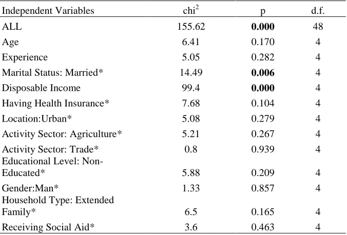
Assumption of parallel regression must be secured in ordered logit models. In many researches this is a disregarded hypothesis. In detecting poverty affecting factors subsequent to model estimation in order to explore the validity of parallel regression hypothesis, Wald test suggested by Brant (1990) has been conducted and obtained findings are reported in Table 3.
According to the result of Wald test (significant chi-square value) parallel regression hypothesis are rejected. Test result shows that marital status and usable income variables in particular (bold in the table) are, based on parallel regression hypothesis, problematic. Other variables on the other hand do not deviate from the hypothesis. Since in ordered logit model parallel regression assumption failed, generalized logit model has been estimated. In estimating generalized ordered logit model at first, restricted model that provided parallel regression assumption and unrestricted model that does not verify parallel regression assumption have been estimated. Later in order to decide which to choose from the two analyzed models, LR test has been conducted the results of which are summarized in Table 4.
186 estimation of unrestricted model is better. Thus,
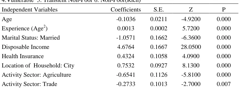
generalized ordered logit model was estimated according to unrestricted model. The results of generalized order logit model are reported in Table 5.
Estimated coefficients of generalized order logit model cannot directly be interpreted hence in order to interpret the coefficients of model, marginal effects have been calculated. In Table 5, marginal effect values are given in the columns placed next to each estimated coefficient.
To summarize, obtained generalized ordered logit model results show that an increase of 1% in the age of head of household brings about an increase (%) in extremely poor, chronically poor, poor, vulnerable (under risk of poverty) , transient non-poor households whereas it has the opposite effect over rich class. An increase of 1% in disposable income alleviates the risk of poverty by 0.01518% while increases the chance of richness (non-poor) by 1.16505%. As the variables of experience and educational level are analyzed it surfaces that both variables have lessening effect on poverty within the first 5 categories while in the last category it has an accelerating effect on the possibility of richness. In year 2009, an increase of 1% in state of being married increased the likelihood of extreme poverty by 0.00227% while for rich (non-poor) class, the chance of richness decreased by 0.25139%. An increase of 1% in possessing private health insurance alleviated the risk of extreme poverty while it enhanced the potentiality of richness. Employment of head of household in agriculture and trade sector, in comparison with service, manufacturing, construction sectors, for the 5 categories had rising effect on the likelihood of poverty and lessening effect on the chance of richness. The families receiving social aids, compared to the ones not receiving any, are close to poverty risk but distant away from richness chance. As for year 2009, an increase of 1% in crowded families accelerated the likelihood of poverty by 0.00570% in poor classes whereas in rich class it decreased the chance of being rich by 0.26393%. While it has a lessening effect on the poverty risk of urban
settlers in the rich class, the last category, it had positive effects.1
Conclusion
Poverty rephrase globally common concept affecting both developed and developing countries for centuries. The new identity of poverty as a global threat has forced national and international organizations and governments to work on remedial policies. In current research, by using year 2009 household budget survey data, the factors that affected poverty in that year and its dimensions have been explored. Obtained findings can be summarized such:
In poor class and middle class age of head of household increases the risk of poverty while in rich class young age accelerates the chance of richness. The rise in experience, disposable income, educational level accelerates the chance of richness.
In 2009, being married, compared to singleness, increased the risk of poverty and alleviated the chance of richness.
Families with private health insurance, compared to others, are distant away from the risk of poverty.
In 2009, the ones employed in agriculture and trade sectors were, compared to other sectors, closer to the risk of poverty.
In 2009, households receiving social aids were, compared to non receivers, closer to the risk of poverty.
As the size of household expands the chance of richness falls down.
In 2009, rural settlers were closer to poverty than urban settlers.
Finally as the gender variable is analyzed it has been determined that men are, compared to women, closer to the risk of poverty. Gender variable
1 Detailed interpretations of coefficients can be requested
187 has failed to verify the expected
impact in present research.
In line with above listed results it has been observed that dependent variable divided into 6 categories has performed the same tendency for the first 5 classes -the poor and the middle- while in the 6th class namely the rich(non-poor) there has been significant diversions in the direction and magnitude of coefficients. It has been observed that there is a difference between
5th class (transient not-poor) and non-poor (the rich). The findings of current research demonstrate that in our country middle class has gradually approached the poor classes and the gap between the middle and the rich class has widened. To concluded, this finding underlines the necessity to take immediate measurements and work on remedial policies.
Table 1. Definition of Independent Variables
Demographic Variables Age (year)
Experience (year)
Marital Status (Married:1, Single:0)
Educational Level (Non educated:0, Other:1) Gender (Male:1, Female:0)
Social Status Variables Health Insurance (Yes:1,No:0) Social Aid (Yes:1, No:0)
Logarithmic Usable Income (TL)
Variables Indicating the Employed Sector of Head of Household
Agriculture:1, Other:0 Trade:1, Other:0
(Other: Manufacturing, Construction, Service).
Household features Household Type (Crowded Family:1, Other:0) Household Size
Table 2. Results of Ordered Logit Model
N:3462 LR chi2(12)=2106.25 Prob > chi2=0.000 Log Likelihood=-3521.66 Pseudo R2=0.2302
Dependent Variable: The Categories of
Poverty
1: Extremely Poor 2. Cronically Poor 3.Poor
4.Vulnerable 5. Transient Non-Poor 6. Non-Poor(Rich)
Independent Variables Coefficients S.E. Z P
Age -0.1036 0.0211 -4.9200 0.000
Experience (Age2) 0.0013 0.0002 5.7200 0.000
Marital Status: Married -1.0571 0.1662 -6.3600 0.000
Disposable Income 4.6764 0.1667 28.0500 0.000
Health Insurance 0.4324 0.1058 4.0900 0.000
188 Educational Level: Uneducated -0.9429 0.1296 -7.2700 0.000
Gender: Man -0.3033 0.1127 -2.6900 0.007
Household Type: Extended Family -1.1469 0.0950 -12.0700 0.000
Receiving Social Aid: -1.0795 0.2090 -5.1600 0.000
/τ1 | 11.3669 0.7515
/ τ2 | 13.0251 0.7503
/ τ3 | 14.2529 0.7548
/ τ4 | 15.2369 0.7599
/ τ5 | 17.2085 0.7736
Notes: Basic Categories; Unmarried, Not having Health Insurance, Urban, Educated, Not Extended Family, Not Receiving Social Aid, Manufacturing/Construction/Services τ: Cut Points, S.E.: Standart Error, p: Probability
Table 3: Results of Wald Test
Independent Variables chi2 p d.f.
ALL 155.62 0.000 48
Age 6.41 0.170 4
Experience 5.05 0.282 4
Marital Status: Married* 14.49 0.006 4
Disposable Income 99.4 0.000 4
Having Health Insurance* 7.68 0.104 4
Location:Urban* 5.08 0.279 4
Activity Sector: Agriculture* 5.21 0.267 4
Activity Sector: Trade* 0.8 0.939 4
Educational Level:
Non-Educated* 5.88 0.209 4
Gender:Man* 1.33 0.857 4
Household Type: Extended
Family* 6.5 0.165 4
Receiving Social Aid* 3.6 0.463 4
Notes: df, Degree of Freedom * shows base categories.
Table 4: Results of LR Test
Likelihood-ratio test LR chi2(48) 58.29
189 Table 5: Results of Generalized Ordered Logit Model
Generalized Ordered Logit Model N =3462 Dependent Variable: The Categories of Poverty
Log Likelihood=-3521.6554 LR chi2(60) = 2106.25 1.Extremely Poor 4.Vulnerable
Prob > chi2 =0.0000 Pseudo R2 =0.2302 2.Chronically Poor 5.Transient Non-Poor 3.Poor 6.Non-Poor(Rich)
Coefficient Marginal Effect Coefficient
Marginal Effect Coefficient
Marginal Effect Coefficient
Marginal Effect Coefficient
Marginal Effect Coefficient
Marginal Effect
Variables
(Householder Characteristics) β dy/dx β dy/dx β dy/dx β dy/dx β dy/dx β dy/dx
-0.104 0.00034 -0.104 0.00138 -0.104 0.00370 -0.104 0.00672 -0.104 0.01368 - -0.02581 -0.021 -0.00008 -0.021 -0.0003 -0.021 -0.00079 -0.021 0.001411 -0.021 0.0028472 - 0.00524 0.001 -0.000004 0.001 -0.00002 0.001 -0.00005 0.001 -0.00008 0.001 -0.00002 - 0.00032 0.000 0.00000 0.000 0.00000 0.000 0.00001 0.000 0.00002 0.000 0.00003 - 0.00006
Marital Status
-1.057 0.00227 -1.057 0.00943 -1.057 0.02601 -1.057 0.05093 -1.057 0.16274 - -0.25139 0.166 0.00041 0.166 0.00129 0.166 0.00318 0.166 0.00618 0.166 0.02616 - 0.03504 4.676 -0.01518 4.676 0.06236 4.676 -0.16686 4.676 -0.30321 4.676 -0.61744 - 1.16505 0.167 0.00224 0.167 0.00582 0.167 0.01168 0.167 0.01849 0.167 0.03689 - 0.04171
Health Insurance
0.432 -0.00167 0.432 -0.00681 0.432 -0.01783 0.432 -0.03079 0.432 -0.04842 - 0.10553 0.106 0.00054 0.106 0.00204 0.106 0.00510 0.106 0.00830 0.106 0.00983 - 0.02503
Location
0.753 -0.00280 0.753 -0.01144 0.753 -0.02999 0.753 -0.05204 0.753 -0.08744 - 0.18370 0.093 0.00057 0.093 0.00189 0.093 0.00448 0.093 0.00720 0.093 0.01008 - 0.02183
Activity Sector
-0.654 0.00253 -0.654 0.01032 -0.654 0.02695 -0.654 0.04632 -0.654 0.07296 - -0.15909 0.113 0.00063 0.113 0.00226 0.113 0.00557 0.113 0.00895 0.113 0.01054 - 0.02632 -0.273 0.00098 -0.273 0.00400 -0.273 0.01058 -0.273 0.01871 -0.273 0.03322 - -0.06748 0.101 0.00042 0.101 0.00166 0.101 0.00428 0.101 0.00735 0.101 0.01128 - 0.02470
Educational Level
-0.943 0.00463 -0.943 0.01862 -0.943 0.04674 -0.943 0.07353 -0.943 0.07477 - -0.21830 0.130 0.00111 0.130 0.00389 0.130 0.00894 0.130 0.01203 0.130 0.00621 - 0.02645
Gender
-0.303 0.00089 -0.303 0.00367 -0.303 0.00991 -0.303 0.01843 -0.303 0.04280 - -0.07569 0.113 0.00032 0.113 0.00127 0.113 0.00342 0.113 0.00646 0.113 0.01685 - 0.02803
Household Type
-1.147 0.00570 -1.147 0.02288 -1.147 0.05705 -1.147 0.08869 -1.147 0.08961 - -0.26393 0.095 0.00105 0.095 0.00326 0.095 0.00696 0.095 0.00915 0.095 0.00718 - 0.01925
Social Aids From Government
-1.080 0.00612 -1.080 0.02436 -1.080 0.05941 -1.080 0.08779 -1.080 0.06269 - -0.24037 0.209 0.00204 0.209 0.00754 0.209 0.01660 0.209 0.01949 0.209 0.00927 - 0.03807 Standart Errors are denoted under the coefficients and marginal effects.* shows basic categories.
All coefficients and marginal effects are significant at the five percent level.
Transient Non-Poor Non-Poor(Rich)
Urban*
Extremely Poor Chronically Poor Poor Vulnerable
Age
Experience(Age Squared)
Married*
Disposable Income
Having Health Insurance*
Agriculture*
Trade*
Non-Educated*
Male*
Extended Family*
Receiving Social Aids*
References
Aranz J. M. and Canto O. (2011) ‘‘Measuring The Effect of Spell Recurrence on Poverty Dynamics-Evidence from Spain’’, Journal of Economic Inequality, Vol. 9, pp .1-27.
Bartram D. (2011) ‘‘Economic Migration and Hapiness: Comparing Immigrants and Natives
Hapiness Gains from Income’’, Social Indicators Research, Vol. 103, pp.57-76.
190 Bustillo, Rafal, M. and Anton Hose,I. (2011)
‘‘From Rags to Riches? Immigration and Poverty in Spain’’, Population Research and Policy Review,Vol.30, No.5, pp.661-676.
Coromaldi, M. and Zoli, M. (2011) ‘‘Deriving Multidimensional Poverty Indicators: Methodological Issues and Emprical Analysis for Italy’’, Social Indicators Research,Vol.104, No.1. pp: 1-18.
Cruces G.,and Wodon, Q. (2007) ‘‘Risk-Adjusted Poverty in Argentina: Measurement and Determinants’’, Journal of Development Studies, Vol. 43, No.7, pp .1189-1214.
Cuesta J., Nopo H. and Pizzolitto G., (2011) ‘‘Using Pseudo Panels toMeasure Income Mobility in Latin America’’, Review of Income and Wealth, Vol.57, No. 2 ,pp.224-246.
Dağdemir Özcan (1999) ‘‘Türkiye Ekonomisinde Yoksulluk Sorunu ve Yoksulluğun Analizi:1987-1994’’, Hacettepe İktisadi İdari Bilimler Fakültesi Dergisi, Vol.17, No.1, pp.23-40.
Dansuk Ercan (1997) ‘‘Türkiye de Yoksulluğun Ölçülmesi ve Sosyoekonomik Yapılarla Ölçülmesi’’,Sosyal Sektörler ve Koordinasyon Genel Müdürlüğü Ücretler ve Gelirler Dairesi Başkanlığı, Devlet Planlama Teşkilatı.
Desai M; and Shai A. (1988) ‘‘An Econometric Approach to the Measurement of Poverty’’, Oxford Economic Papers, Vol.40, No.3 , pp.505-522.
Deutsch J.; Silber, J.(2005) ‘‘Measuring Multidimensional Poverty: An Emprical Comparison of Various Approaches’’, Review of Income and Wealth, Vol. 51, No.1, pp.145-174.
Dimitry S.(2003) ‘‘Below the Poverty Line :Duration Of Poverty in Russia’’, Economics Education and Research Consortium Working Paper Series, No.03/04.
Dumanlı Recep (2002) ‘‘Türkiye'de Yoksulluk Sınırı ve Boyutları”in Yoksullukla Mücadele Stratejileri, Ed. Aktan C.C., Hak-İş Konfederasyonu Yayınları, Ankara.
Finnie R., Sweetman A. (2003) ‘‘Poverty Dynamics: Empirical Evidence for Canada’’, Canadian Journal of Economics, Vol.36, No.2, pp.291-325.
Fisher M.,(2007) ‘‘Why is US poverty higher in Non Metropolitan than Metropolitan Areas?
’’ , Growth and Change, Vol.38, No.1, pp.56-76.
Fourage D. and Layte R. (2003) ‘‘Duration of Poverty Spells of Europe’’, EPAG Working Papers Number 2003-47.
Geda A., Jong N. , Mwangi K., Mwabu G. (2001) ‘‘Determinants of Poverty in Kenya:A Household Level Analysis’’, KIPPRA Discussion Paper, No.9.
Gerry, J. G. and Li C. A. (2010) ‘‘Consumption Smoothing and Vulnerability in Russia’’, Applied Economics ,Vol.42, No.16, pp.1995-2007.
Kızılgöl Ö. ve Demir Ç. (2010) ‘‘Türkiye'de Yoksulluğun Boyutuna İlişkin Ekonometrik Analizler’’, İşletme ve Ekonomi Araştırmaları Dergisi, Vol.1, No.1 ; pp.21-32.
Kolev, A. (2005) ‘‘Unemployment, Job Quality and Poverty:A case study of Bulgaria’’, International Labour Review, Vol.144, No. 1, pp. 85–114.
Long, J. Scott (1997)‘‘Regression Models For Categorical And Limited Dependent Variables’’, Sage Publications, California. McCulloch, N. and Baulch, B. (2000) ‘‘Simulating The Impact of Policy Upon Chronic and Transitory in Rural Pakistan’’, Journal of Develeopment Studies, Vol.36, No.6, pp.100-130.
Moreno S.P.,(2010) ‘‘Financial Development and Poverty in Developing Countries: A Casual Analysis’’, Empirical Economics,Vol.41, No.1 pp.57-80.
Nashgold , F.( 2009) ‘‘Microeconomic Determinants of Income Equality in Rural Pakistan’’, Journal of Development Studies Vol. 45, No.5, pp.746-768.
Oshio T.; Kobayashi M.,(2011) ‘‘Area Level Income and Individual Happiness:Evidence From Japan’’, Journal of Hapiness Studies, Vol.12, No.4, pp.633-649.
Robone S.,Jones A.R. and Rice N.(2011) ‘‘Contractual Conditions, Working Conditions and Their Impact on Health and Well Being’’, The European Journal of Health Economics, Vol.12, No.5, pp.429-444.
191 Smith K., (2003) ‘‘Individual Welfare in the
Soviet Union’’, Social Indicators Research, Vol. 64, No. 1 pp.75-105.
Şengül S ve Cafri R.(2010) ‘‘Yoksulluk Ölçümünde Engel ve Rothbarth Eşdeğerlik Ölçekleri’’, Çukurova Üniversitesi Sosyal Bilimler Enstitüsü Dergisi, Vol.19, No.2, pp.47-61.
Tzadivis, N.,Salvati, Pratesi M. and Chambers, R.,(2008) ‘‘M-Quantile Models with Application Poverty Mapping’’, Statistical Methods and Applications ,Vol.17, No.3, pp.393-411.
Wagle, U. R. (2009)‘‘Capability Deprivation and Income Poverty in the United States, 1994 and 2004:Measurement Outcomes and Demographic Profiles’’, Social Indicators Research. , Vol.94, No.3, pp.509-533.
Wang, P. and Vander Weele, J. T.,(2011) ‘‘Emprical Research on Factors Related to the subjective Well-Being of Chinese Urban Residents’’, Social Indicators Research, Vol. 101, No.3, pp.447-459.
Worldbank(2000) ‘‘World Development Report (WDR) 2000/2001: Attacking Poverty’’, WB, Washington DC.